AMO Quantum Simulators

Short Definition

Atomic, molecular, and optical (AMO) quantum simulators use controlled atoms, ions, molecules, photons, and collective excitations to reproduce selected quantum models and processes. Three especially mature families are ultracold gases in optical lattices, trapped-ion simulators, and neutral-atom arrays coupled through Rydberg states.

The platforms do not differ only by engineering convenience. They expose different native degrees of freedom, interaction graphs, preparation routes, observables, and dominant errors. A platform comparison is meaningful only after the target model and scientific output have been specified.

Canonical Scope

This page is the canonical home for the cross-platform simulation workflow:

• matching target degrees of freedom to AMO encodings;
• deriving the effective Hamiltonian from laboratory controls;
• comparing optical-lattice, trapped-ion, and Rydberg-array capabilities;
• identifying state-preparation, measurement, and validation obligations;
• accounting for platform-specific model errors and resources; and
• stating what an AMO experiment has established about the target model.

Detailed platform physics remains canonical elsewhere:

• Optical Lattices develops recoil scales, bands, Wannier functions, loading, and calibration;
• Trapped-Ion Control develops sidebands, spin-dependent forces, motional gates, and errors;
• Rydberg Blockade develops pair interactions, finite blockade, collective excitation, and gates;
• Optical Tweezers develops loading, rearrangement, transport, and imaging; and
• the hardware pages on trapped-ion qubits and neutral-atom and Rydberg qubits own processor architecture and scaling.

This page instead asks: given a model and observable, what does each AMO route actually implement, and what evidence supports the correspondence?

There Is No Platform Winner in the Abstract

An optical lattice naturally supplies periodic motion, exchange statistics, and local interactions for itinerant particles. Trapped ions naturally supply highly controlled effective spins, collective bosonic modes, long-range couplings, and individual readout. Rydberg arrays naturally supply reconfigurable geometry, strong state-dependent interactions, kinetic constraints, and site-resolved snapshots.

Those strengths are complementary. A large atom count does not compensate for an unknown temperature. Near-perfect ion readout does not make an incorrectly eliminated phonon harmless. A programmable tweezer geometry does not turn a $1/r^6$ interaction into an arbitrary coupling matrix. The useful question is whether the platform’s native physics matches the target contract closely enough for the desired observable.

Write the Simulation Contract First

The minimum contract contains six layers.

Target model

Specify the Hilbert space, geometry, boundary conditions, Hamiltonian or channel, and parameter regime. For example,

$$H_{\mathrm{tar}} = \sum_{i<j}J_{ij}Z_iZ_j + B\sum_iX_i + \sum_i h_iZ_i.$$

A name such as “Ising model” is insufficient. The interaction range, signs, longitudinal fields, dimensionality, and boundary conditions can change the physics qualitatively.

Encoding map

State which physical levels, occupations, modes, or positions represent the target degrees of freedom. An encoding map

$$\mathcal E: \mathcal H_{\mathrm{tar}} \longrightarrow \mathcal H_{\mathrm{lab}}$$

should identify the intended subspace and the states counted as leakage.

Effective dynamics

Derive a laboratory Hamiltonian in that subspace,

$$P H_{\mathrm{lab}} P = \lambda H_{\mathrm{tar}} + \delta H,$$

where $P$ projects onto the encoding, $\lambda$ converts target time to laboratory time, and $\delta H$ contains unwanted interactions and parameter errors. Terms removed by a rotating frame, perturbative elimination, or time averaging require their own validity conditions.

Preparation and protocol

Specify the initial state or ensemble, ramps, quenches, periodic drives, measurements, and postselection. Ground-state preparation, thermal-state sampling, real-time evolution, and spectroscopy are different tasks even when they use the same Hamiltonian.

Observable map

For every target observable $O$, state the laboratory estimator $O_{\mathrm{lab}}$ and the processing needed to infer it:

$$\langle O\rangle_{\mathrm{tar}} \longleftrightarrow \mathbb E[\widehat O_{\mathrm{lab}}].$$

The arrow may include basis rotations, parity reconstruction, loss correction, Fourier transforms, thermometry, or response-function inversion.

Evidence and tolerance

Name the time window, parameter range, observable precision, and confidence level. Include convergence or robustness checks against the relevant control, cutoff, temperature, finite-size, decoherence, and sampling errors.

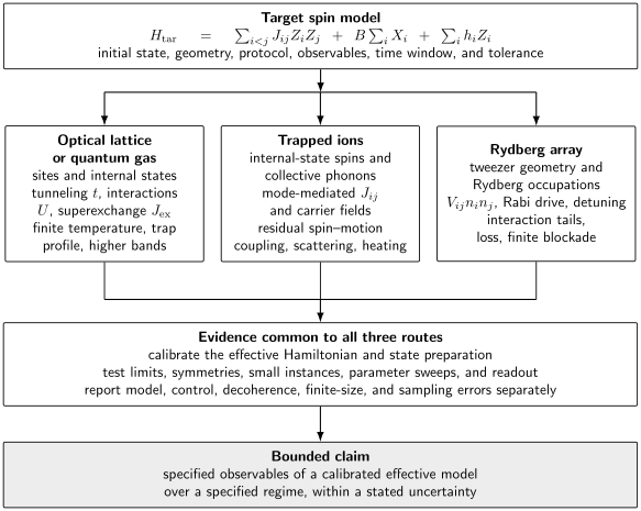
The same target symbols have different laboratory meanings. The useful comparison is between complete model-to-control-to-evidence pipelines, not between particle counts alone.

Platform Crosswalk

Question	Optical lattices and gases	Trapped ions	Rydberg arrays
Native degrees of freedom	Mobile bosons or fermions, internal states	Internal-state spins, collective phonons	Local occupations or spins in tweezer geometries
Common models	Bose–Hubbard, Fermi–Hubbard, spin exchange, synthetic gauge fields	Long-range Ising/XY/Heisenberg, spin–boson, digital blocks	Ising, XY exchange, blockade-constrained models, gauge encodings
Interaction structure	Contact interactions plus tunneling; usually local in real space	Mode-mediated, often dense and approximately power law	Geometry-set van der Waals or dipolar interactions
Preparation strength	Natural quantum gases and many-body cooling	High-fidelity product states and local control	Rearranged low-entropy product arrays and programmable geometry
Readout strength	Momentum distributions; microscopy can be site resolved	High-efficiency site-resolved spin readout	Site-resolved snapshots with loss and state-detection caveats
Central bottleneck	Entropy, thermometry, inhomogeneity, heating	Mode spectrum, control errors, scaling, residual motion	Rydberg lifetime, finite blockade, interaction tails, loss
Natural simulation mode	Mostly analog, with Floquet and local digital elements	Analog, digital, and hybrid	Analog and digital–analog, with growing circuit capability

This table describes tendencies, not immutable boundaries. Species, trap geometry, control architecture, and the scientific task matter more than the platform label.

Optical Lattices and Ultracold Gases

Optical-lattice simulators retain the particles’ center-of-mass motion. They are therefore a natural route to itinerant many-body models rather than merely arrays of stationary qubits.

From continuum matter to a lattice model

For one species in an external optical potential, a common microscopic model is

$$H = \int d^dr\, \Psi^\dagger(\mathbf r) \left[ -\frac{\hbar^2\nabla^2}{2m} +V_{\mathrm{lat}}(\mathbf r) +V_{\mathrm{trap}}(\mathbf r) \right] \Psi(\mathbf r) +H_{\mathrm{int}}.$$

Expanding the field in lowest-band Wannier orbitals,

$$\Psi(\mathbf r) \approx \sum_i w_i(\mathbf r)a_i,$$

gives a Hubbard-type model when higher bands, long-range tunneling, and nonlocal interactions are controlled.

For bosons,

$$H_{\mathrm{BH}} = -t\sum_{\langle i,j\rangle} (a_i^\dagger a_j+a_j^\dagger a_i) + \frac U2\sum_i n_i(n_i-1) + \sum_i\epsilon_i n_i.$$

For two-component fermions,

$$H_{\mathrm{FH}} = -\sum_{\langle i,j\rangle,\sigma} t_{ij,\sigma} (c_{i\sigma}^\dagger c_{j\sigma}+\mathrm{h.c.}) + U\sum_i n_{i\uparrow}n_{i\downarrow} + \sum_{i,\sigma}\epsilon_{i\sigma}n_{i\sigma}.$$

The parameters are overlap integrals, not labels attached directly to laser knobs. For example,

$$t_{ij} = -\int d^dr\, w_i^*(\mathbf r) H_0 w_j(\mathbf r),$$

while a contact interaction gives schematically

$$U = g\int d^dr\,|w_i(\mathbf r)|^4.$$

Calibrating lattice depth, scattering length, Wannier functions, and trap inhomogeneity is therefore part of establishing the simulated Hamiltonian.

Effective spin models

At one particle per site and strong repulsion,

$$\frac tU\ll1,$$

virtual doublon–hole processes generate spin exchange. For the repulsive two-component Fermi–Hubbard model at half filling, the leading scale is

$$J_{\mathrm{ex}} = \frac{4t^2}{U}.$$

The low-energy model is antiferromagnetic Heisenberg exchange up to higher orders and inhomogeneities. This mapping imposes two competing timescales:

$$\tau_t\sim\frac\hbar t, \qquad \tau_{\mathrm{ex}}sim\frac{\hbar U}{4t^2}.$$

Making $U/t$ very large improves charge-sector separation but slows the spin dynamics, allowing heating and loss more time to act. “Deeper in the Mott regime” is not automatically better for every observable.

State-dependent lattices, Raman coupling, Floquet modulation, dipolar atoms or molecules, and Rydberg dressing can extend the available spin and gauge interactions. Each extension also adds off-resonant couplings, micromotion, long-range terms, or dissipation that must be quantified.

State preparation is an entropy problem

Loading a cold gas into a lattice is approximately adiabatic only relative to the relevant many-body gaps and relaxation pathways. The final temperature is not generally obtained by carrying the free-gas temperature through unchanged. Entropy can redistribute across charge, spin, edge, and trap degrees of freedom.

For a thermal target,

$$\rho_\beta = \frac{e^{-\beta H}}{Z}, \qquad Z=\operatorname{Tr}e^{-\beta H},$$

the inverse temperature $\beta$ is a fitted physical parameter with model dependence and uncertainty. Thermometry based on density fluctuations, correlations, equation-of-state data, or comparison with classical numerics should identify the regime in which the thermometer is valid.

Observables

Common measurements include:

• time-of-flight momentum distributions and interference peaks;
• band mapping and excitation spectroscopy;
• density profiles and equations of state;
• doublon fractions and parity-projected occupations;
• spin and density structure factors;
• site-resolved snapshots from quantum-gas microscopes;
• connected correlations and full counting statistics; and
• quench, transport, and response dynamics.

A microscope image is not automatically a snapshot of the target occupation. Light-assisted collisions may project doublons to parity, imperfect freezing can move particles, and reconstruction algorithms have a confusion matrix.

Optical-lattice error ledger

Track at least:

$$\epsilon_{\mathrm{lat}} \leftarrow \left\lbrace \begin{array}{l} \text{band truncation and long-range hopping},\\ \text{trap and lattice inhomogeneity},\\ \text{finite temperature and preparation entropy},\\ \text{interaction and lattice-depth calibration},\\ \text{photon-scattering and technical heating},\\ \text{particle loss and detection reconstruction},\\ \text{finite size and boundary conditions}. \end{array} \right.$$

The ultracold-atom quantum-simulation frontier tracks which many-body regimes are established and which remain active.

Trapped-Ion Simulators

Trapped-ion simulators encode effective spins in long-lived internal states and use collective motion as a controllable interaction bus. Their natural graph is set by normal modes and optical forces rather than by physical nearest-neighbor contact.

Spin–motion starting point

Let ion $i$ couple to normal mode $m$ with Lamb–Dicke factor $\eta_{im}$. A bichromatic spin-dependent force can be written schematically in an interaction picture as

$$H_{\mathrm{SDF}}(t) = \hbar\sum_{i,m} g_{im}\sigma_i^\phi \left( a_m e^{-i\delta_m t} + a_m^\dagger e^{i\delta_m t} \right).$$

When spin–motion entanglement remains perturbative or closes at the relevant times, eliminating the phonons gives

$$H_{\mathrm{spin}} \approx \sum_{i<j}J_{ij} \sigma_i^\phi\sigma_j^\phi + \sum_i\mathbf B_i\cdot\boldsymbol\sigma_i.$$

The coupling matrix is a weighted mode sum. One representative dependence is

$$J_{ij} \propto \Omega_i\Omega_j \sum_m \eta_{im}\eta_{jm} \frac{\omega_m}{\mu^2-\omega_m^2},$$

where $\mu$ is the force beat-note scale and $\Omega_i$ are optical coupling amplitudes. Exact prefactors and signs depend on the drive convention.

In suitable regimes, the measured couplings are summarized by

$$J_{ij} \approx \frac{J_0}{|i-j|^\alpha}, \qquad 0\lesssim\alpha\lesssim3.$$

The power law is an approximation to a finite mode-generated matrix. A simulation should report the measured $J_{ij}$ or its residual from the fit, especially near boundaries or when individual mode contributions dominate.

Native model families

Spin-dependent forces and coherent rotations naturally support:

• transverse-field Ising models;
• XY and XXZ interactions through frame changes or multiple drives;
• frustrated and long-range spin models;
• Floquet and digital–analog sequences;
• spin–boson and vibronic models retaining selected phonons;
• monitored and dissipative maps using optical pumping and measurement; and
• digital simulation through high-fidelity gate primitives.

Retaining phonons as target modes and eliminating them as a bus are opposite modeling choices. A mode cannot be both an ignored mediator and a target bath degree of freedom without a clear partition.

Preparation and observables

Optical pumping and coherent rotations give low-entropy product states. Slow ramps, variational controls, digital circuits, and engineered dissipation can prepare correlated states. Fluorescence readout typically supplies site-resolved samples in a chosen spin basis; pre-rotations expose other Pauli components.

For a sampled bit string $s=(s_1,\ldots,s_N)$, diagonal correlators follow from

$$\langle Z_{i_1}\cdots Z_{i_k}\rangle \approx \frac1{N_{\mathrm{shot}}} \sum_{r=1}^{N_{\mathrm{shot}}} s_{i_1}^{(r)}\cdots s_{i_k}^{(r)}.$$

Readout confusion, leakage, and loss still require calibration. The ability to read every ion does not remove the exponential cost of full state tomography.

Trapped-ion error ledger

Track at least:

$$\epsilon_{\mathrm{ion}} \leftarrow \left\lbrace \begin{array}{l} \text{coupling-matrix calibration},\\ \text{residual spin--motion entanglement},\\ \text{Lamb--Dicke and rotating-wave corrections},\\ \text{motional heating and mode-frequency drift},\\ \text{laser intensity, phase, and addressing errors},\\ \text{spontaneous scattering and qubit dephasing},\\ \text{state-preparation and measurement errors}. \end{array} \right.$$

For analog dynamics, the mode spectrum and force detuning are model data, not only gate-calibration details.

Rydberg-Array Simulators

Neutral atoms in optical tweezers can be imaged, rearranged into programmable geometries, initialized in internal states, and coupled strongly through Rydberg excitation. The mapping is especially direct for interacting spin and constraint models.

Driven Rydberg Hamiltonian

For one ground state $\lvert g\rangle$ and one Rydberg state $\lvert r\rangle$, define

$$n_i = \lvert r_i\rangle\langle r_i\rvert = \frac{I+Z_i}{2}.$$

In a rotating frame, a common model is

$$H_{\mathrm R} = \sum_i \left( \frac{\hbar\Omega_i}{2}X_i - \hbar\Delta_i n_i \right) + \sum_{i<j}V_{ij}n_i n_j.$$

For van der Waals interactions,

$$V_{ij} \approx \frac{C_6}{r_{ij}^6},$$

away from pair resonances and anisotropies that invalidate a scalar $C_6$ description. Resonant exchange between suitable Rydberg levels can instead produce dipolar $1/r^3$ couplings and XY-type spin exchange.

Exact Ising rewrite

Substituting $n_i=(I+Z_i)/2$ gives, up to a constant,

$$H_{\mathrm R} = \sum_{i<j}\frac{V_{ij}}4Z_iZ_j + \sum_i\frac{\hbar\Omega_i}{2}X_i + \sum_i h_i^{\mathrm{eff}}Z_i,$$

with

$$h_i^{\mathrm{eff}} = -\frac{\hbar\Delta_i}{2} + \frac14\sum_{j\ne i}V_{ij}.$$

Thus the interaction-generated longitudinal field is part of the mapping. A uniform laser detuning does not necessarily yield a uniform effective field on a finite or irregular array. Local detunings or edge compensation may be needed.

Blockade-constrained dynamics

If nearest-neighbor double excitation is strongly off resonant, projection onto the blockade subspace gives the idealized chain Hamiltonian

$$H_{\mathrm{PXP}} = \frac{\hbar\Omega}{2} \sum_i P_{i-1}X_iP_{i+1} - \hbar\Delta\sum_i n_i,$$

where

$$P_i=I-n_i.$$

Finite blockade allows forbidden pairs with small but nonzero amplitude, and interactions beyond the blockade radius remain. The PXP model is therefore an effective target whose leakage and long-range corrections should be measured, not an exact description produced by drawing exclusion circles.

Preparation and snapshots

Tweezer loading is probabilistic, so fluorescence imaging and rearrangement are used to prepare a chosen occupied geometry. After internal-state initialization, quenches and detuning or Rabi-frequency sweeps implement dynamical and quasi-adiabatic protocols.

Many experiments infer a Rydberg excitation because an atom is absent in a final fluorescence image. If ground-state atoms can also be lost, the raw binary variable combines physical excitation with detection loss. A calibrated confusion model might have

$$\Pr(d=1\mid r)=1-\epsilon_{r\to g}, \qquad \Pr(d=1\mid g)=\epsilon_{g\to r},$$

where $d=1$ denotes the detector label assigned to a Rydberg excitation. The inference should propagate uncertainty in both error rates.

Rydberg-array error ledger

Track at least:

$$\epsilon_{\mathrm{Ry}} \leftarrow \left\lbrace \begin{array}{l} \text{position and interaction calibration},\\ \text{finite blockade and long-range tails},\\ \text{Rydberg decay and intermediate-state scattering},\\ \text{Doppler shifts, laser phase noise, and inhomogeneity},\\ \text{atom loss, leakage, and detection confusion},\\ \text{ramp diabaticity and finite-size geometry},\\ \text{model reduction to selected Rydberg levels}. \end{array} \right.$$

The dated Rydberg Array Frontiers page tracks current scale and research claims separately from this stable mapping workflow.

Worked Cross-Platform Benchmark: One Ising Target

Consider

$$H_{\mathrm{tar}} = \sum_{i<j}J_{ij}^{\mathrm{tar}}Z_iZ_j + B^{\mathrm{tar}}\sum_iX_i + \sum_i h_i^{\mathrm{tar}}Z_i.$$

The goal is not to declare three implementations identical, but to expose the transformations and residuals needed for a fair comparison.

Optical-lattice route

Encode a spin in two internal states at one particle per site. Superexchange generically produces an XXZ-type model,

$$H_{\mathrm{XXZ}} = \sum_{\langle i,j\rangle} \left[ J_\perp(S_i^xS_j^x+S_i^yS_j^y) + J_zS_i^zS_j^z \right] + \sum_i\mathbf b_i\cdot\mathbf S_i.$$

State-dependent tunneling, interaction anisotropy, gradients, and periodic driving may isolate or emphasize the desired Ising term. The residual exchange $J_\perp$, higher-order terms of scale $t^3/U^2$ or smaller depending on the process, trap inhomogeneity, and thermal defects belong in $\delta H$.

This route is attractive when mobile particles, exchange statistics, or the Hubbard parent model are part of the science. It is less direct when an arbitrary dense Ising coupling matrix is the sole target.

Trapped-ion route

Choose the spin-dependent-force axis so the native interaction is $\sum J_{ij}^{\mathrm{ion}}X_iX_j$, then rotate spin axes globally if the target uses $Z_iZ_j$. Carrier or microwave drives supply the transverse field.

The comparison uses the measured matrix, not merely a fitted exponent:

$$J_{ij}^{\mathrm{ion}} = \lambda J_{ij}^{\mathrm{tar}} + \delta J_{ij}^{\mathrm{ion}}.$$

Individual addressing and pulse modulation can reshape the matrix, but the normal-mode structure, available optical power, and off-resonant excitation constrain which matrices are practical.

Rydberg route

Choose tweezer positions and a Rydberg level so that

$$\frac{V_{ij}}4 = \lambda J_{ij}^{\mathrm{tar}} + \delta J_{ij}^{\mathrm{Ry}}.$$

Set

$$\frac{\hbar\Omega_i}{2} = \lambda B^{\mathrm{tar}}$$

and compensate the interaction-induced field with

$$-\frac{\hbar\Delta_i}{2} + \frac14\sum_{j\ne i}V_{ij} = \lambda h_i^{\mathrm{tar}}.$$

Geometry gives powerful but structured programmability. A Euclidean $1/r^6$ matrix obeys geometric constraints and cannot represent every signed coupling graph without dressing, Floquet sequences, encodings, or digital operations.

Compare coupling matrices after optimizing time scale

Let $J^{\mathrm{lab}}$ denote the calibrated off-diagonal coupling matrix. A useful dimensionless residual is

$$\epsilon_J = \min_{\lambda>0} \frac{ \|J^{\mathrm{lab}}-\lambda J^{\mathrm{tar}}\|_F }{ \|\lambda J^{\mathrm{tar}}\|_F }.$$

The least-squares scale is

$$\lambda_* = \frac{ \operatorname{Tr}[(J^{\mathrm{tar}})^TJ^{\mathrm{lab}}] }{ \|J^{\mathrm{tar}}\|_F^2 },$$

provided the positive-scale constraint is satisfied. Report local-field and unwanted-operator residuals separately; a small $\epsilon_J$ does not certify the complete Hamiltonian.

Propagate Hamiltonian mismatch to an observable

If

$$\widetilde H = \lambda H_{\mathrm{tar}}+\delta H,$$

then for the same initial state and bounded observable $O$, a general short-time bound is

$$\left| \langle O(t)\rangle_{\widetilde H} - \langle O(\lambda t)\rangle_{H_{\mathrm{tar}}} \right| \le \frac{2t}{\hbar} \|O\|_\infty \|\delta H\|_infty.$$

The bound is often pessimistic because it is global. Observable-specific perturbation theory, locality bounds, measured sensitivity, and parameter sweeps can be much tighter. It nevertheless makes one point unavoidable: small coupling residuals accumulate with simulation time.

State Preparation Across Platforms

State preparation is part of the simulated problem, not a preface to it.

Product states

Trapped ions and rearranged tweezer arrays can prepare many product states with local control. Optical lattices naturally prepare occupation and spin patterns through cooling, filtering, gradients, and local addressing, but defects and thermal ensembles can be central.

Ground states by ramps

For a parameter path $H(s)$ completed in time $T$, adiabatic intuition depends on the minimum relevant gap,

$$\Delta_{\min} = \min_s [E_1(s)-E_0(s)].$$

A sufficient scaling estimate contains

$$T \gg \hbar \max_s \frac{ |\langle1(s)|\partial_sH|0(s)\rangle| }{ \Delta(s)^2 }.$$

In many-body systems the gap can shrink with size, while decoherence and heating favor shorter ramps. An observed low energy or high order parameter does not by itself prove ground-state preparation.

Thermal and generalized ensembles

Optical-lattice gases often begin as thermodynamic ensembles; ion and Rydberg experiments more often sample pure-state dynamics and obtain effective thermal behavior through subsystems or long-time observables. In every case, test the ensemble claim with more than one fitted observable when possible.

Dissipative preparation

Optical pumping, sympathetic cooling, lossy modes, and measurement feedback can engineer open-system dynamics. The target generator and hardware noise must be separated using the workflow in Open-System Simulation.

Measurement and Inference

AMO platforms often produce repeated microscopic samples rather than direct wavefunctions. An estimator should be defined before data collection.

Correlations

For binary outcomes $z_i=\pm1$,

$$C_{ij} = \langle z_i z_j\rangle - \langle z_i\rangle\langle z_j\rangle.$$

The structure factor is

$$S(\mathbf q) = \frac1N \sum_{i,j} e^{i\mathbf q\cdot(\mathbf r_i-\mathbf r_j)} C_{ij}.$$

Position uncertainty, missing particles, parity projection, or a readout confusion matrix alters this estimator. Corrections should be validated on known states and propagated to the covariance of $S(\mathbf q)$.

Dynamical response

Quenches and weak probes can estimate spectral functions and susceptibilities. A finite observation window $T$ limits frequency resolution to a scale of order

$$\delta\omega \gtrsim \frac{2\pi}{T},$$

before windowing, decoherence, and sampling are considered. Fourier peaks are not infinitely sharp eigenenergies.

Entanglement witnesses and tomography

Collective observables, randomized measurements, classical shadows, and local tomography can witness or estimate selected entanglement properties. Full tomography remains exponential. Every entanglement claim should state the measured witness, assumptions, finite-sample correction, and robustness to SPAM errors.

Calibration as Hamiltonian Learning

A simulator is calibrated by estimating the effective model actually realized, not only by setting control voltages to design values.

Static calibration

Measure single-particle spectra, Rabi frequencies, interaction shifts, mode frequencies, tunneling, on-site interactions, light shifts, trap profiles, and readout matrices as appropriate. Report spatial distributions and drift, not only global means.

Dynamical calibration

Use few-body oscillations, Ramsey phases, correlation propagation, blockade leakage, normal-mode response, or modulation spectroscopy to infer couplings. Fit several initial states or observables to reduce identifiability problems.

Closed-loop validation

Reserve data not used in parameter fitting. A model that reproduces its calibration traces can still fail on a different state, time, or observable. Out-of-sample prediction is stronger evidence than an in-sample residual.

Verification Ladder

Trust should be built from overlapping checks.

1. Unit tests: one particle, one ion, one pair, zero interaction, or zero drive.
2. Few-body tests: exact spectra and dynamics with all measured nuisance parameters included.
3. Symmetry tests: conserved particle number, parity, magnetization, or gauge constraints where the target requires them.
4. Parameter convergence: lattice depth, force detuning, blockade ratio, time step, ramp duration, system size, and sampling.
5. Cross-observable tests: fit one observable and predict another.
6. Cross-method tests: exact diagonalization, tensor networks, Monte Carlo where sign-free, kinetic theory, or independent hardware.
7. Limiting regimes: weak/strong coupling, high temperature, short time, integrable points, and decoupled subsystems.
8. Blind predictions: pre-register parameters or withhold data when a high-stakes beyond-classical claim is made.

Cross-platform agreement is valuable because platforms have different error mechanisms. It is not automatically independent if both analyses use the same unverified effective model or fitting assumptions.

Resource Accounting

AMO resource tables should go beyond particle count.

Resource	Optical lattice	Trapped ions	Rydberg array
Active degrees of freedom	Occupied sites, spin components, bands	Spins and retained phonon modes	Loaded atoms, internal/Rydberg levels
Geometry	Lattice plus trap envelope	Ion crystal and mode graph	Measured tweezer coordinates
Energy hierarchy	Band gaps, $t$, $U$, temperature	Mode gaps, force detunings, $J_{ij}$	Rabi frequencies, detunings, $V_{ij}$
Preparation	Entropy, filling, defects, ramp time	Cooling, optical pumping, circuit/ramp depth	Loading, rearrangement, loss, ramp depth
Coherent budget	Heating time and many-body scales	Laser coherence and motional heating	Ground/Rydberg coherence and lifetime
Readout	Collection, parity or state fidelity	Per-ion confusion and leakage	Loss/excitation confusion and imaging fidelity
Sampling	Images or shots per setting	Shots per basis and time	Snapshots per geometry and time
Classical work	Band/model inference, thermometry	Pulse/mode optimization, fitting	Rearrangement, geometry optimization, inference

For a dynamical claim, a useful dimensionless depth is the number of target interaction times reached before decoherence,

$$Q_{\mathrm{sim}} = \frac{\tau_{\mathrm{coh}}}{\tau_{\mathrm{int}}}, \qquad \tau_{\mathrm{int}} \sim \frac\hbar{J_{\mathrm{char}}}.$$

This is not a universal quality metric. It omits preparation, control inhomogeneity, observable sensitivity, and whether $J_{\mathrm{char}}$ is the relevant many-body scale. It is useful only with the full ledger.

Error Ledger

A platform-neutral accounting scaffold is

$$\epsilon_{\mathrm{tot}} \lesssim \epsilon_{\mathrm{enc}} + \epsilon_{\mathrm{eff}} + \epsilon_{\mathrm{prep}} + \epsilon_{\mathrm{ctrl}} + \epsilon_{\mathrm{open}} + \epsilon_{\mathrm{meas}} + \epsilon_{\mathrm{finite}} + \epsilon_{\mathrm{stat}}.$$

Here:

• $\epsilon_{\mathrm{enc}}$ measures leakage outside the intended encoding;
• $\epsilon_{\mathrm{eff}}$ measures truncation and unwanted Hamiltonian terms;
• $\epsilon_{\mathrm{prep}}$ covers entropy, defects, and diabaticity;
• $\epsilon_{\mathrm{ctrl}}$ covers calibration, drift, and pulse errors;
• $\epsilon_{\mathrm{open}}$ covers decoherence, loss, and heating;
• $\epsilon_{\mathrm{meas}}$ covers readout and inference bias;
• $\epsilon_{\mathrm{finite}}$ covers size, boundaries, and observation time;
• $\epsilon_{\mathrm{stat}}$ covers finite shots and fitted parameters.

The additive form is a planning device. Correlated errors, nonlinear inference, and postselection require joint propagation or end-to-end synthetic data tests.

Common Mistakes

Comparing platform size without comparing the task

One thousand stored atoms, one hundred interacting spins, and fifty individually controlled ions are not interchangeable resources. Report which degrees of freedom participate, for how long, under which controls, and with which observables.

Calling a design Hamiltonian the measured Hamiltonian

Laser settings and trap geometries imply a model only after calibration and approximations. Use measured $t$, $U$, $J_{ij}$, $V_{ij}$, fields, and residuals where available.

Ignoring state preparation

A correct Hamiltonian acting on an unknown thermal or defective state does not answer a ground-state question. Treat temperature, filling, leakage, and ramp fidelity as model parameters.

Treating a fitted power law as an exact ion interaction

Ion couplings are finite mode sums. Report the coupling matrix and fit residual, not only $J_0$ and $\alpha$.

Treating blockade as a hard geometric rule

Finite interaction shifts, detuning, linewidth, and pulse bandwidth determine double-excitation leakage. Long-range tails survive outside a nominal blockade radius.

Equating an optical-lattice depth with a Hubbard ratio

$t/U$ depends on Wannier functions, scattering parameters, dimensionality, and additional confinement. Lattice depth alone does not specify the many-body Hamiltonian.

Correcting readout without propagating calibration uncertainty

Inverting a confusion matrix can amplify variance and systematic error. Bootstrap or jointly infer calibration and physics parameters when necessary.

Claiming a phase from one order parameter

Finite systems and ramps can show large order parameters without establishing thermodynamic order, topological order, or equilibrium. Combine correlations, scaling, spectroscopy, and preparation diagnostics appropriate to the claim.

Treating classically hard as scientifically verified

The failure of one classical method is not validation. Beyond-classical experiments need internal consistency, overlapping tractable regimes, independent methods, and transparent uncertainty.

Reporting Checklist

A mature AMO quantum-simulation report should state:

• target Hamiltonian or process, geometry, boundaries, and convention;
• encoding and leakage definition;
• microscopic laboratory model and effective-model derivation;
• calibrated parameters, spatial variation, drift, and covariance;
• initial-state preparation, temperature or purity, filling, and defects;
• protocol timing, ramps, drives, and retained bath modes;
• observable estimators and all reconstruction or postselection;
• system size, active-particle count, interaction graph, and coherence budget;
• platform-specific error ledger and convergence tests;
• classical and cross-platform benchmarks;
• exact scope of any quantum-advantage claim; and
• data, code, calibration records, and analysis provenance.

Key Results

1. AMO platforms realize effective models, not bare target symbols; the model-to-control derivation is part of the result.
2. Optical lattices are naturally suited to itinerant particles, Hubbard models, exchange physics, and thermodynamic ensembles.
3. Trapped ions are naturally suited to programmable long-range spins, retained bosonic modes, and high-efficiency local measurements.
4. Rydberg arrays are naturally suited to reconfigurable spin geometries, strong interactions, and blockade-constrained dynamics.
5. Temperature and entropy, residual spin–motion coupling, and finite blockade are platform-defining errors rather than incidental nuisances.
6. The same Ising target maps to different controls and unwanted terms on each platform.
7. Particle count alone is not a simulation resource metric.
8. Trust rests on calibrated effective dynamics, known preparation, explicit estimators, convergence, and independent validation.

Research Status

Optical-lattice realizations of Bose–Hubbard and Fermi–Hubbard physics, site-resolved quantum-gas microscopy, trapped-ion spin models with tunable long-range interactions, and programmable Rydberg Ising arrays are established. Experiments have observed many-body ordering, correlation spreading, nonequilibrium dynamics, constrained dynamics, and selected gauge-theory phenomena across these platforms.

Active research includes lower-entropy doped Hubbard regimes, larger and more programmable ion coupling graphs, coherent spin–boson simulation, Rydberg models beyond simple Ising constraints, digital–analog protocols, error-aware long-time dynamics, and verification after classical simulation becomes inconclusive. Broad, application-relevant quantum advantage is not a settled property of any AMO platform; it remains specific to a task, observable, comparison set, and error budget.

References

1. R. P. Feynman, “Simulating Physics with Computers,” International Journal of Theoretical Physics 21, 467 (1982), doi:10.1007/BF02650179.
2. J. I. Cirac and P. Zoller, “Goals and Opportunities in Quantum Simulation,” Nature Physics 8, 264 (2012), doi:10.1038/nphys2275.
3. I. M. Georgescu, S. Ashhab, and F. Nori, “Quantum Simulation,” Reviews of Modern Physics 86, 153 (2014), doi:10.1103/RevModPhys.86.153.
4. I. Bloch, J. Dalibard, and W. Zwerger, “Many-Body Physics with Ultracold Gases,” Reviews of Modern Physics 80, 885 (2008), doi:10.1103/RevModPhys.80.885.
5. I. Bloch, J. Dalibard, and S. Nascimbène, “Quantum Simulations with Ultracold Quantum Gases,” Nature Physics 8, 267 (2012), doi:10.1038/nphys2259.
6. C. Gross and I. Bloch, “Quantum Simulations with Ultracold Atoms in Optical Lattices,” Science 357, 995 (2017), doi:10.1126/science.aal3837.
7. D. Jaksch et al., “Cold Bosonic Atoms in Optical Lattices,” Physical Review Letters 81, 3108 (1998), doi:10.1103/PhysRevLett.81.3108.
8. M. Greiner et al., “Quantum Phase Transition from a Superfluid to a Mott Insulator in a Gas of Ultracold Atoms,” Nature 415, 39 (2002), doi:10.1038/415039a.
9. W. S. Bakr et al., “Probing the Superfluid-to-Mott Insulator Transition at the Single-Atom Level,” Science 329, 547 (2010), doi:10.1126/science.1192368.
10. A. Mazurenko et al., “A Cold-Atom Fermi–Hubbard Antiferromagnet,” Nature 545, 462 (2017), doi:10.1038/nature22362.
11. R. Blatt and C. F. Roos, “Quantum Simulations with Trapped Ions,” Nature Physics 8, 277 (2012), doi:10.1038/nphys2252.
12. D. Porras and J. I. Cirac, “Effective Quantum Spin Systems with Trapped Ions,” Physical Review Letters 92, 207901 (2004), doi:10.1103/PhysRevLett.92.207901.
13. K. Kim et al., “Quantum Simulation of Frustrated Ising Spins with Trapped Ions,” Nature 465, 590 (2010), doi:10.1038/nature09071.
14. J. W. Britton et al., “Engineered Two-Dimensional Ising Interactions in a Trapped-Ion Quantum Simulator with Hundreds of Spins,” Nature 484, 489 (2012), doi:10.1038/nature10981.
15. J. Zhang et al., “Observation of a Many-Body Dynamical Phase Transition with a 53-Qubit Quantum Simulator,” Nature 551, 601 (2017), doi:10.1038/nature24654.
16. A. Browaeys and T. Lahaye, “Many-Body Physics with Individually Controlled Rydberg Atoms,” Nature Physics 16, 132 (2020), doi:10.1038/s41567-019-0733-z.
17. H. Bernien et al., “Probing Many-Body Dynamics on a 51-Atom Quantum Simulator,” Nature 551, 579 (2017), doi:10.1038/nature24622.
18. S. Ebadi et al., “Quantum Phases of Matter on a 256-Atom Programmable Quantum Simulator,” Nature 595, 227 (2021), doi:10.1038/s41586-021-03582-4.
19. G. Semeghini et al., “Probing Topological Spin Liquids on a Programmable Quantum Simulator,” Science 374, 1242 (2021), doi:10.1126/science.abi8794.
20. P. Hauke et al., “Can One Trust Quantum Simulators?” Reports on Progress in Physics 75, 082401 (2012), doi:10.1088/0034-4885/75/8/082401.
21. K. Sun et al., “Quantum Simulation of Spin-Boson Models with Structured Bath,” Nature Communications 16, 4042 (2025), doi:10.1038/s41467-025-59296-y.
22. D. González-Cuadra et al., “Observation of String Breaking on a (2 + 1)D Rydberg Quantum Simulator,” Nature 642, 321 (2025), doi:10.1038/s41586-025-09051-6.

Further Connections

• Simulation of Lattice Models
• Analog Quantum Simulation
• Digital Quantum Simulation
• Hybrid Quantum Simulation
• Device Characterization
• Reporting Standards

Exercises

Exercise 1: Rydberg-to-Ising mapping

Starting from

$$H = \sum_i \left( \frac{\hbar\Omega_i}{2}X_i - \hbar\Delta_i n_i \right) + \sum_{i<j}V_{ij}n_i n_j,$$

use $n_i=(I+Z_i)/2$ to derive the Ising coupling, effective longitudinal field, and constant energy shift.

Solution

The one-body term becomes

$$-\hbar\Delta_i n_i = -\frac{\hbar\Delta_i}{2}I - \frac{\hbar\Delta_i}{2}Z_i.$$

For each pair,

$$V_{ij}n_i n_j = \frac{V_{ij}}4 (I+Z_i+Z_j+Z_iZ_j).$$

Collecting terms gives

$$H = E_0I + \sum_{i<j}\frac{V_{ij}}4Z_iZ_j + \sum_i\frac{\hbar\Omega_i}{2}X_i + \sum_i h_i^{\mathrm{eff}}Z_i,$$

where

$$h_i^{\mathrm{eff}} = -\frac{\hbar\Delta_i}{2} + \frac14\sum_{j\ne i}V_{ij}$$

and

$$E_0 = -\frac\hbar2\sum_i\Delta_i + \frac14\sum_{i<j}V_{ij}.$$

The constant affects only a global phase in closed-system dynamics.

Exercise 2: Superexchange timescale

A half-filled repulsive Fermi–Hubbard simulator has $U/t=8$. Express the superexchange scale in units of $t$ and compare the tunneling and exchange timescales. What happens to the exchange time if $U/t$ is doubled at fixed $t$?

Solution

The leading exchange is

$$J_{\mathrm{ex}} = \frac{4t^2}{U} = \frac{4t}{8} = \frac t2.$$

Thus

$$\tau_t = \frac\hbar t, \qquad \tau_{\mathrm{ex}} = \frac\hbar{J_{\mathrm{ex}}} = 2\frac\hbar t.$$

At $U/t=16$, $J_{\mathrm{ex}}=t/4$ and $\tau_{\mathrm{ex}}=4\hbar/t$. Doubling $U$ improves perturbative charge separation but doubles the laboratory time required for a fixed amount of exchange dynamics.

Exercise 3: Best time-rescaling factor

Minimize

$$f(\lambda) = \|J^{\mathrm{lab}}-\lambda J^{\mathrm{tar}}\|_F^2$$

over unconstrained real $\lambda$. Derive $\lambda_*$ and state what to do if the comparison permits only $\lambda>0$ but the unconstrained optimum is negative.

Solution

Expand the Frobenius norm:

$$f(\lambda) = \|J^{\mathrm{lab}}\|_F^2 - 2\lambda \operatorname{Tr} [(J^{\mathrm{tar}})^TJ^{\mathrm{lab}}] + \lambda^2 \|J^{\mathrm{tar}}\|_F^2.$$

Setting the derivative to zero gives

$$\lambda_* = \frac{ \operatorname{Tr}[(J^{\mathrm{tar}})^TJ^{\mathrm{lab}}] }{ \|J^{\mathrm{tar}}\|_F^2 }.$$

If $\lambda_*$ is negative but only forward positive time rescaling is allowed, the constrained infimum occurs at the boundary $\lambda\to0^+$. That signals that the measured coupling pattern is anticorrelated with the target and should not be described as the same simulator with a positive time conversion. A sign-changing frame transformation may help only if it is explicitly valid for the full Hamiltonian and geometry.

Exercise 4: Finite blockade leakage

Two identical atoms are resonantly driven with single-atom Rabi frequency $\Omega$. The doubly excited state is detuned by an interaction shift $V$. Using off-resonant-coupling intuition, estimate the scaling of its population in the strong-blockade regime and name two effects that make the estimate incomplete.

Solution

The singly excited bright state couples to the doubly excited state with a matrix element of order $\hbar\Omega$. An off-resonant amplitude therefore scales as

$$|a_{rr}| \sim \frac{\hbar\Omega}{V},$$

so the double-excitation probability scales as

$$P_{rr} \sim \left| \frac{\hbar\Omega}{V} \right|^2.$$

The prefactor depends on pulse shape and collective matrix elements. Detuning, finite linewidth, Doppler shifts, pair-state mixing, anisotropy, spontaneous decay, and the pulse bandwidth can all modify the estimate. The blockade ratio must be tested under the actual protocol.

Exercise 5: Ion coupling residual

A three-ion simulator has measured couplings

$$J^{\mathrm{lab}}_{12}=1.00, \qquad J^{\mathrm{lab}}_{23}=0.94, \qquad J^{\mathrm{lab}}_{13}=0.20,$$

in common units. The target nearest-neighbor chain has couplings $(1,1,0)$. Compute the best positive scale and the relative Frobenius residual using the three independent off-diagonal entries.

Solution

Treat the independent entries as vectors

$$\mathbf j_{\mathrm{lab}} = (1.00,0.94,0.20), \qquad \mathbf j_{\mathrm{tar}} = (1,1,0).$$

Then

$$\lambda_* = \frac{1.00+0.94}{2} = 0.97.$$

The squared residual is

$$\|\mathbf j_{\mathrm{lab}} - \lambda_*\mathbf j_{\mathrm{tar}}\|_2^2 = 0.03^2+(-0.03)^2+0.20^2 = 0.0418.$$

The target norm after scaling is

$$\|\lambda_*\mathbf j_{\mathrm{tar}}\|_2 = 0.97\sqrt2.$$

Therefore

$$\epsilon_J = \frac{\sqrt{0.0418}}{0.97\sqrt2} \approx 0.149.$$

The unwanted end-to-end coupling dominates the mismatch.

Exercise 6: Readout correction

A Rydberg detector reports $d=1$ with probability $0.96$ for a true Rydberg atom and with probability $0.03$ for a true ground-state atom. If the observed fraction of $d=1$ outcomes is $0.42$, estimate the true Rydberg population.

Solution

Let $p_r$ be the true Rydberg population. Then

$$p_{\mathrm{obs}} = 0.96p_r+0.03(1-p_r) = 0.03+0.93p_r.$$

Hence

$$p_r = \frac{0.42-0.03}{0.93} \approx 0.419.$$

This point estimate is close to the raw fraction because the two error contributions nearly balance here. A real analysis must propagate uncertainty in both calibration probabilities and account for correlated loss if present.

Exercise 7: Finite observation window

An experiment records a correlation function for $T=8\hbar/J$. Estimate the Fourier-bin spacing in units of $J/\hbar$. Explain why quoting a spectral peak to much higher precision is not justified from this record alone.

Solution

The natural angular-frequency spacing is

$$\delta\omega \sim \frac{2\pi}{T} = \frac\pi4\frac J\hbar \approx 0.785\frac J\hbar.$$

Windowing and model-based fitting can interpolate a peak location, but that precision then depends on assumptions about line shape, noise, decay, and the number of components. The finite record alone does not resolve arbitrary nearby frequencies, and decoherence generally broadens the response further.

Exercise 8: Choose a platform

For each task below, identify a natural first-choice AMO platform and one important caveat: (a) the equilibrium equation of state of a two-dimensional Fermi–Hubbard gas, (b) a tunable long-range Ising quench with local spin readout, and (c) constrained dynamics on a programmable two-dimensional graph.

Solution

(a) An ultracold Fermi gas in an optical lattice is the natural first choice because fermionic motion, on-site repulsion, and thermodynamic density profiles are native. The central caveats are entropy and thermometry, together with trap inhomogeneity and Hubbard-parameter calibration.

(b) A trapped-ion simulator is a natural first choice because mode-mediated Ising couplings can be long ranged and individual fluorescence readout is strong. The measured coupling matrix may differ from a pure power law, and residual spin–motion entanglement and optical errors must be bounded.

(c) A Rydberg tweezer array is a natural first choice because the geometry is reconfigurable and blockade supplies strong kinetic constraints. Finite blockade, $1/r^6$ tails, Rydberg decay, and loss-versus-excitation readout must be included.

These are starting points, not uniqueness claims. A task may favor another platform after its required size, interaction graph, observables, and error budget are specified.