Simulation of Lattice Models

Short Definition

Quantum simulation of a lattice model is the use of a controlled quantum device to prepare, evolve, or interrogate a finite spin, fermion, boson, or constrained model whose degrees of freedom and interactions are organized by a graph or spatial lattice. A reproducible simulation specifies the finite instance, encoding, state, evolution or solver, observable, accuracy target, and evidence used to validate the answer.

The short Hamiltonians associated with lattice models can hide a long computational specification. A statement such as “simulate the Hubbard model” does not yet fix the cluster, boundaries, filling, mode order, fermion map, state, time window, observable, or meaning of the requested precision. Those choices can change both the physics and the circuit by orders of magnitude.

Canonical Scope

This page owns the finite-lattice-to-processor workflow:

• completing a finite spin, fermion, or boson target from graph and boundary data;
• encoding local spaces, particle statistics, truncations, and constraints;
• preserving useful locality through term grouping, routing, and hardware placement;
• selecting digital, analog, or hybrid preparation and evolution;
• measuring local, correlation, spectral, and phase-sensitive quantities;
• budgeting finite-size, truncation, algorithmic, hardware, and sampling errors;
• verifying a computation in tractable limits and validating the physical conclusion drawn from it.

The Lattice Models Overview owns the general definition and physical interpretation of lattice models. Dedicated pages own the physics, conventions, exact limits, and phase structure of the Transverse-Field Ising Model, Heisenberg Model, Hubbard Model, and Bose–Hubbard Model. Simulation of Quantum Materials owns the additional model-reduction and material-validation layers needed to make claims about a real substance. General evolution algorithms remain at Hamiltonian Simulation, Trotter–Suzuki Methods, and Qubitization and Quantum Signal Processing.

The Central Principle: Preserve Locality End to End

Locality is not merely a property of the formula written by the theorist. It must survive four representations:

1. model locality: each term acts on a bounded region of the lattice;
2. encoding locality: that term maps to an operator of manageable support on the register;
3. hardware locality: the required register interactions fit the device graph with limited routing;
4. observable locality: the requested output can be estimated without reconstructing an exponentially large state.

A nearest-neighbor fermion hopping term can become a long Pauli string after a poor mode ordering. A local spin interaction can require many SWAPs on a mismatched processor. Conversely, a globally defined quantity such as a structure factor may still be efficiently assembled from repeated local measurements. The correct resource estimate follows the entire chain, not the first Hamiltonian alone.

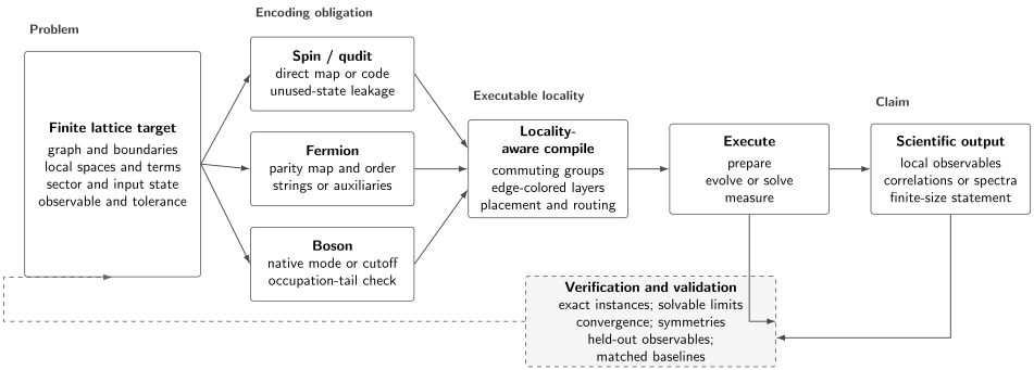
A lattice simulation is an observable-level pipeline. Graph, boundaries, sector, and target state complete the finite problem. Spin, fermion, and boson encodings create different locality and leakage obligations. Term layers and routing expose the executable structure; preparation, evolution, and measurement produce a claim only after convergence and independent checks.

Specify a Finite Simulation Contract

A useful contract is

$$\mathcal T_L = \left( G_L, \{\mathcal H_x\}, H_L, \mathcal C, \rho_0, \mathcal Q, \epsilon, 1-\alpha \right).$$

Here $G_L$ is the finite interaction graph, $\mathcal H_x$ is the local space at site, link, or cell $x$, $H_L$ is the finite Hamiltonian, and $\mathcal C$ contains exact constraints and the chosen symmetry sector. The input state or ensemble is $\rho_0$, while $\mathcal Q$ specifies the requested quantities, times, frequencies, or parameter points. The result must meet error tolerance $\epsilon$ with confidence or success probability at least $1-\alpha$.

Geometry and support

Write the Hamiltonian as a sum over supports,

$$H_L = \sum_{X\subseteq G_L} h_X,$$

and record the sites on which each $h_X$ acts. For a finite-range model, one usually has

$$\operatorname{diam}(X)\le R, \qquad \lVert h_X\rVert\le J_0,$$

with interaction range $R$ and local scale $J_0$ independent of system size. This support list, rather than a model nickname, determines parallel layers, commutators, routing, and oracle cost.

Boundaries are part of the Hamiltonian

Open, periodic, twisted, cylindrical, and irregular boundaries define different finite operators. For a nearest-neighbor ring,

$$H_{\mathrm{PBC}} = \sum_{j=1}^{L-1}h_{j,j+1} +h_{L,1},$$

whereas the open chain omits $h_{L,1}$. The wrapping term is geometrically local on the target ring even if it is nonlocal on a linear processor. This is a routing fact, not permission to omit the term. Boundary conventions and finite-size consequences are treated in Boundary Conditions on Lattices.

Sector and initial condition

State all exact charges used to restrict the calculation. Typical examples are total magnetization, particle number, fermion parity, momentum, and point group quantum numbers. Also distinguish:

$$\rho_0 = \lvert\psi_0\rangle\langle\psi_0\rvert, \qquad \rho_\beta = \frac{e^{-\beta H_L}}{Z_L},$$

because a pure-state quench and a thermal calculation are different tasks even when they use the same Hamiltonian.

Observable and normalization

A local expectation, extensive sum, and intensive density carry different precision requirements. If

$$O_{\mathrm{tot}}=\sum_{x=1}^{L}O_x, \qquad o_L=\frac{O_{\mathrm{tot}}}{L},$$

then fixed additive error in $O_{\mathrm{tot}}$ becomes increasingly strict per site, while fixed error in $o_L$ defines a stable bulk target. State which quantity is reported and whether the intended conclusion concerns this finite instance or a thermodynamic extrapolation.

Representative Model Families

The following Hamiltonians illustrate different compilation obligations. They do not replace their canonical model pages.

Family	Representative terms	Natural register issue	Typical outputs
Ising	$Z_iZ_j$, $X_i$, longitudinal fields	direct qubit map; edge scheduling	magnetization, domains, gaps, quenches
Heisenberg or XXZ	$X_iX_j+Y_iY_j+\Delta Z_iZ_j$	exchange compilation; spin symmetry	correlators, transport, structure factors
Fermi–Hubbard	$c_{i\sigma}^\dagger c_{j\sigma}+\mathrm{h.c.}$, $n_{i\uparrow}n_{i\downarrow}$	anticommutation, mode order, routing	densities, spin correlations, Green functions
Bose–Hubbard	$b_i^\dagger b_j+\mathrm{h.c.}$, $n_i(n_i-1)$	local occupation cutoff or native modes	number statistics, coherence, expansion

For example, a transverse-field Ising family can be written

$$H_{\mathrm I} = -\sum_{(i,j)\in E}J_{ij}Z_iZ_j -\sum_i h_iX_i.$$

The isotropic spin-$1/2$ Heisenberg family is

$$H_{\mathrm H} = \frac14 \sum_{(i,j)\in E}J_{ij} \left( X_iX_j+Y_iY_j+Z_iZ_j \right).$$

A spinful Hubbard instance is

$$\begin{aligned} H_{\mathrm F} ={}& -\sum_{(i,j),\sigma} t_{ij} \left( c_{i\sigma}^\dagger c_{j\sigma} +c_{j\sigma}^\dagger c_{i\sigma} \right) \\ &+ U\sum_i n_{i\uparrow}n_{i\downarrow} -\sum_{i,\sigma}\mu_{i\sigma}n_{i\sigma}. \end{aligned}$$

A truncated Bose–Hubbard instance begins from

$$H_{\mathrm B} = -\sum_{(i,j)}t_{ij} \left( b_i^\dagger b_j+b_j^\dagger b_i \right) +\frac{U}{2}\sum_i n_i(n_i-1) -\sum_i\mu_i n_i.$$

The letters $L$, $E$, $J$, $t$, $U$, and $\mu$ are not enough to reproduce a calculation. One must still provide graph orientation, coefficient units, operator normalization, boundaries, local cutoffs, and sector data.

Encode the Local Degrees of Freedom

Spin-1/2 sites

One physical or logical qubit per site is the simplest exact mapping,

$$\lvert\downarrow\rangle_i\leftrightarrow\lvert0\rangle_i, \qquad \lvert\uparrow\rangle_i\leftrightarrow\lvert1\rangle_i.$$

The choice can be reversed, but it must be stated because signs of magnetization and bitstring interpretation depend on it. A direct map preserves the support of every Pauli interaction. It does not guarantee low cost if the device coupling graph differs from the target graph.

Higher spins and qudits

A local dimension $q$ can use a native qudit, a binary encoding with $\lceil\log_2q\rceil$ qubits, or a unary encoding with $q$ basis states spread over $q$ qubits and a one-hot constraint. Binary encoding minimizes qubit count but can make local operators denser. Unary encoding uses more qubits but often turns transitions between adjacent levels into low-weight operations.

If $2^m>q$ for a binary register, the unused states form a leakage space. With $P$ the projector onto valid states, a simulation should report at least

$$p_{\mathrm{valid}} = \operatorname{Tr}(P\rho), \qquad p_{\mathrm{leak}}=1-p_{\mathrm{valid}}.$$

Postselecting invalid states changes the sampling cost and must not be hidden.

Fermionic modes

Fermionic occupation has finite local dimension, but anticommutation requires parity bookkeeping. For an ordered set of modes and the convention that $\lvert1\rangle_j$ is occupied, Jordan–Wigner gives

$$c_j = \left( \prod_{k<j}Z_k \right) \frac{X_j+iY_j}{2}.$$

Consequently, for $p<q$, a hopping operator contains the intervening parity string,

$$c_p^\dagger c_q+c_q^\dagger c_p = \frac12 \left( X_p Z_{p+1}\cdots Z_{q-1}X_q + Y_p Z_{p+1}\cdots Z_{q-1}Y_q \right).$$

The derivation, occupation convention, and boundary signs belong to Jordan–Wigner Transformation. For simulation, the key consequence is that mode order is a compilation choice. Serpentine order can keep many bonds short on a rectangular lattice, but no one-dimensional ordering keeps every two-dimensional nearest-neighbor bond adjacent. Auxiliary-qubit and locality-preserving encodings trade extra registers and constraints for shorter operator support.

Fermionic SWAP networks provide another strategy: move modes through one another while applying interactions when the relevant pair becomes adjacent. The logical layout then changes during the circuit, so the compiler must track which qubit currently represents each mode. An ordinary SWAP and a fermionic SWAP differ by the sign on the doubly occupied state.

Bosonic modes

A qubit register cannot exactly hold the infinite basis of an ideal bosonic mode. A local cutoff retains

$$\mathcal H_i^{(n_{\max})} = \operatorname{span} \left\{ \lvert0\rangle, \ldots, \lvert n_{\max}\rangle \right\},$$

with dimension $q=n_{\max}+1$. The truncated creation operator is

$$b_i^\dagger = \sum_{n=0}^{n_{\max}-1} \sqrt{n+1} \lvert n+1\rangle\langle n\rvert.$$

This is a new finite model, not an exact representation of the unbounded one. Convergence requires increasing $n_{\max}$ and monitoring upper-level weight, for example

$$p_{\mathrm{edge},i} = \langle n_{\max}\rvert\rho_i\lvert n_{\max}\rangle.$$

A small mean occupation alone is not a cutoff certificate when rare high-occupation events control the observable. Native oscillator platforms can avoid a qubit cutoff at the register level, but finite anharmonicity, detector range, and leakage still impose an operational truncation.

Symmetries and Constraints

An encoding is exact only on its declared physical space. Let $Q_a$ denote conserved charges and $G_x$ local constraints. The ideal target obeys

$$[H_L,Q_a]=0, \qquad G_x\lvert\psi_{\mathrm{phys}}\rangle =g_x\lvert\psi_{\mathrm{phys}}\rangle.$$

Symmetry can reduce qubit count, constrain an ansatz, enable tapering, and provide diagnostics. These are distinct uses. A circuit that commutes with particle number may still leave the intended momentum sector. Postselecting on a measured charge can mitigate detected leakage, but changes the accepted-shot count and does not repair coherent errors within the sector.

For an implemented state $\rho$, report sector leakage through projectors,

$$p_{\mathrm{out}} = 1-\operatorname{Tr}(P_{\mathcal C}\rho),$$

and condition observables only when the conditioning rule and its uncertainty were specified in advance. Symmetry Sectors develops the corresponding block structure for classical many-body methods.

Turn the Interaction Graph into Circuit Layers

The conflict graph

Suppose two-site terms are associated with target edges $e\in E$. Construct a conflict graph whose vertices are the terms and whose edges join terms that cannot execute simultaneously. A proper coloring partitions the Hamiltonian,

$$H_L = \sum_{a=1}^{\chi}H_a, \qquad H_a=\sum_{e\in\mathcal M_a}h_e,$$

where $\mathcal M_a$ is a matching when the only conflict is sharing a site. All gates in one matching can then run in parallel on hardware that supports the corresponding couplings.

For an open nearest-neighbor chain, even and odd bonds suffice:

$$\begin{aligned} H_{\mathrm{odd}} &= h_{1,2}+h_{3,4}+\cdots, \\ H_{\mathrm{even}} &= h_{2,3}+h_{4,5}+\cdots. \end{aligned}$$

An odd periodic ring needs three matching colors, while an even ring needs two. A $D$-dimensional hypercubic nearest-neighbor lattice can be scheduled in $2D$ direction-and-parity layers. These counts describe logical interaction depth; control constraints, crosstalk, and routing can increase physical depth.

Terms need not be disjoint to commute. For example, all Ising bonds $Z_iZ_j$ commute even when they share a site. They may be grouped into one exponential algebraically, yet still require several physical layers because one qubit cannot participate in two simultaneous two-qubit gates. Algebraic grouping and hardware scheduling are related but distinct.

Layout and routing

Let $G_T$ be the target interaction graph and $G_H$ the hardware coupling graph. A placement $\pi:V(G_T)\to V(G_H)$ is useful when most target edges map to short paths. A simple routing burden is

$$C_{\mathrm{route}}(\pi) = \sum_{(i,j)\in E(G_T)} w_{ij} \left[d_H(\pi(i),\pi(j))-1\right],$$

where $d_H$ is hardware graph distance and $w_{ij}$ weights how often the interaction is used. This is only a proxy: parallel congestion, directionality, native gate family, calibration quality, and dynamical remapping also matter.

The wraparound edge of a periodic chain illustrates the issue. It is local in $G_T$. On a linear $G_H$, its endpoints are far apart, so implementing it may require a SWAP network, teleportation, or a different mode layout. Calling the term “nonlocal” without naming the graph conflates model geometry with device geometry.

Keep a layout ledger

For every compiled family, record:

• the target-to-register and register-to-hardware maps;
• the logical identity of each register after every dynamic SWAP layer;
• the number and depth of interaction, routing, and basis-change gates;
• whether periodic bonds, long-range tails, or disorder change the schedule;
• which symmetries each compiled primitive preserves exactly.

This ledger catches a serious fermionic failure mode: measuring the right physical mode on the wrong final qubit after a swap network.

Choose the Simulation Paradigm

Digital execution

A digital simulator represents the target with gates. It is attractive when the model family, boundaries, term strengths, or observables must change frequently. The implementation may use product formulas, randomized formulas, block-encoding methods, qubitization, variational circuits, or phase estimation. These choices have different ancilla, precision, and fault-tolerance requirements.

For a local decomposition $H=\sum_a H_a$, first-order evolution is

$$U_1(\delta t) = \prod_{a=1}^{\chi} e^{-iH_a\delta t},$$

and $r=t/\delta t$ steps approximate $e^{-iHt}$. The leading error depends on commutators between overlapping local terms, not simply on the square of the number of all terms. Locality-aware product-formula bounds can therefore be far tighter than a triangle-inequality estimate that treats every pair as noncommuting.

For geometrically local bounded Hamiltonians, rigorous algorithms can achieve gate count nearly linear in spacetime volume, up to subpolynomial or polylogarithmic factors under their stated assumptions. This is an asymptotic result about encoded local Hamiltonians. State preparation, observable estimation, error correction, and a nonlocal encoding can still dominate an application.

Analog execution

An analog simulator realizes a laboratory generator $H_{\mathrm{lab}}$ whose effective dynamics approximate a target family. Optical lattices naturally realize Hubbard-like motion and interactions; neutral-atom and ion arrays naturally realize programmable spin models. Analog execution can preserve spatial locality without translating every term into gates, but it replaces gate-synthesis error with calibration, unwanted couplings, leakage, and effective-Hamiltonian error.

The target claim needs an explicit map

$$P H_{\mathrm{lab}}P = \lambda H_L+\beta I+\Delta H,$$

where $P$ selects the encoded subspace, $\lambda$ fixes the time scale, $\beta$ is dynamically irrelevant only within that subspace, and $\Delta H$ contains residual terms. Analog Quantum Simulation owns this correspondence and its validation requirements.

Hybrid execution

Hybrid simulation uses a quantum device for a state, overlap, response kernel, or local evolution while a classical loop selects parameters, embeds a cluster, extrapolates size, or reconstructs a spectrum. Examples include variational ground states, quantum-assisted imaginary-time updates, and cluster or embedding workflows. The correct resource is the cost of the whole loop, including failed optimizer iterations and repeated quantum calls.

No paradigm is uniformly best. A native analog array may dominate for broad short-time correlation maps, a shallow digital circuit may be best for a small programmable instance, and fault-tolerant qubitization may win at stringent energy precision. The task contract, not the model label, selects the route.

Prepare the Requested State

Product states and quenches

Computational-basis spin configurations, occupation bitstrings, charge-density waves, domain walls, and Néel states are often inexpensive. They are ideal for quench dynamics because preparation error can be characterized locally and short-time behavior can be checked analytically.

A quench specifies both Hamiltonians,

$$\lvert\psi(t)\rangle = e^{-iH_{\mathrm f}t} \lvert\psi_0(H_{\mathrm i})\rangle.$$

It is not enough to state the final couplings. The initial preparation, quench profile, clock origin, and any ramp time belong to the protocol.

Adiabatic preparation

Choose a path

$$H(s) =(1-s)H_0+sH_1, \qquad s=t/T,$$

or a problem-specific nonlinear schedule. Success depends on the path, minimum relevant gap, matrix elements of $\partial_sH$, degeneracy structure, and endpoint overlap. A large final gap does not rule out an avoided crossing along the path. At a finite-size critical bottleneck, the required time can grow rapidly with $L$.

Symmetry can help or hurt. Remaining in the desired exact sector can avoid irrelevant crossings, but a path that preserves the wrong symmetry cannot reach a target state in another sector. Report the schedule and verify convergence with $T$ rather than labeling a single ramp adiabatic.

Variational preparation

For a parameterized state $\lvert\psi(\boldsymbol\theta)\rangle$, ground-state preparation often minimizes

$$E(\boldsymbol\theta) = \langle\psi(\boldsymbol\theta)\rvert H_L \lvert\psi(\boldsymbol\theta)\rangle.$$

Hamiltonian variational ansätze built from lattice term groups can preserve symmetries and use local gates,

$$U(\boldsymbol\theta) = \prod_{p=1}^{P} \prod_{a=1}^{\chi} e^{-i\theta_{p,a}H_a}.$$

Low energy is not by itself proof of high fidelity when the gap is small or unknown. Optimization bias, estimator noise, ansatz restriction, and hardware error must be separated. VQE owns the general variational algorithm.

Eigenstate filtering and phase estimation

Phase estimation can resolve eigenenergies from an input

$$\lvert\psi_{\mathrm{in}}\rangle = \sum_n c_n\lvert E_n\rangle,$$

but the probability of obtaining $E_n$ is $\lvert c_n\rvert^2$. High-precision evolution does not create overlap with the desired state. Resource estimates must include preparation and repetitions from imperfect overlap. The details belong to Quantum Phase Estimation.

Thermal states

A Gibbs target

$$\rho_\beta = \frac{e^{-\beta H_L}}{\operatorname{Tr}e^{-\beta H_L}}$$

can require purification, imaginary-time methods, probabilistic filtering, open-system engineering, or sampling from a variational ensemble. Low temperature combines ground-state preparation difficulty with entropy and normalization estimation. A state whose energy density matches a thermal value need not reproduce the Gibbs ensemble, especially in integrable or many-body localized regimes.

Evolve Without Losing the Declared Physics

Product-formula structure

For two groups $A+B=H$, the symmetric second-order step is

$$S_2(\delta t) = e^{-iA\delta t/2} e^{-iB\delta t} e^{-iA\delta t/2}.$$

Over fixed total time, its leading global error scales as $O(t\delta t^2)$ times norms of nested commutators under standard bounded-operator assumptions. The constant and size dependence matter. A convergence study should vary $\delta t$, term ordering, and preferably formula order while holding the physical task fixed.

Product formulas can preserve a charge exactly when every compiled group commutes with it:

$$[H_a,Q]=0 \quad\text{for every }a \quad\Longrightarrow\quad [U_1(\delta t),Q]=0.$$

This is stronger than conservation only in the $\delta t\to0$ limit and is a good reason to choose symmetry-respecting groupings.

Local versus global accuracy

Operator-norm accuracy for the entire $L$-site unitary is a strong guarantee. Many scientific tasks ask only for a local observable over finite time. A Lieb–Robinson bound limits the influence of distant perturbations for short-range systems, so an observable-specific simulation can sometimes use a finite causal neighborhood or tolerate errors far outside it. This does not justify discarding distant terms arbitrarily: the truncation radius and resulting error must be derived for the interaction decay, time, and observable.

Long-range interactions

Power-law interactions,

$$J_{ij}\sim\frac{J_0}{r_{ij}^{\gamma}},$$

change term count, scheduling, causal bounds, and analog-model discrepancy. Truncating at radius $R_c$ defines

$$\Delta H_{R_c} = \sum_{r_{ij}>R_c}J_{ij}O_iO_j.$$

Its operator norm can grow with system size even when each omitted coupling is small. Validate the final observable against several cutoffs or include the tail in the target. Never relabel an uncontrolled hardware tail as harmless because the desired textbook model is nearest-neighbor.

Measure the Scientific Output

Local observables and correlations

Single-site polarization and density are

$$m_i^a(t)=\langle\sigma_i^a(t)\rangle, \qquad n_i(t)=\langle\hat n_i(t)\rangle.$$

Connected equal-time correlations remove products of one-point means,

$$C_{ij}^{ab} = \langle O_i^aO_j^b\rangle -\langle O_i^a\rangle \langle O_j^b\rangle.$$

Bitstrings can provide every same-basis $Z$ or number correlator in one shot, but noncommuting bases require additional settings. Covariance between estimators must be retained when many correlators are combined.

Structure factors

For positions $\mathbf r_j$, a static structure factor can be normalized as

$$S^{aa}(\mathbf q) = \frac1L \sum_{i,j} e^{i\mathbf q\cdot(\mathbf r_i-\mathbf r_j)} C_{ij}^{aa}.$$

State whether connected or raw correlations are used and whether $1/L$ or $1/L^2$ normalization is intended. Structure Factors owns the physical interpretation and convention choices.

Dynamical response and spectra

A real-time correlator has the form

$$C_{AB}(t) = \operatorname{Tr} \left[ \rho\,A(t)B(0) \right].$$

Ancilla interferometry, Hadamard tests, direct basis rotations, or linear response to a weak perturbation can estimate its real and imaginary parts. The finite record is windowed before Fourier transformation,

$$\widetilde C_{AB}(\omega) = \int_{-T}^{T} dt\, w(t)e^{i\omega t}C_{AB}(t).$$

Thus frequency resolution, broadening, maximum reliable evolution time, sampling cadence, and window choice are part of the answer. A smooth spectrum can reflect the window rather than intrinsic lifetime. Fermionic Green functions additionally require parity-aware insertion of creation and annihilation operators. Spectral Functions provides the canonical many-body definitions.

Finite systems and order parameters

On a finite system with an exact symmetry, an order parameter odd under that symmetry can have zero expectation in every symmetry eigenstate. For $M=\sum_i Z_i$ and a spin-flip symmetry $P$ satisfying $PMP^\dagger=-M$,

$$P\lvert\psi\rangle=p\lvert\psi\rangle \quad\Longrightarrow\quad \langle M\rangle=0.$$

One instead studies $\langle M^2\rangle$, long-distance correlations, susceptibility, a small symmetry-breaking field with a stated order of limits, or the low-lying finite-size tower. One cluster and one order parameter value do not establish a thermodynamic phase.

Worked Example: Four-Site Ising Quench

Consider an open four-site chain,

$$H = H_Z+H_X,$$

with

$$H_Z = -J \left( Z_1Z_2+Z_2Z_3+Z_3Z_4 \right), \qquad H_X=-h\sum_{j=1}^{4}X_j.$$

Take $\lvert\psi_0\rangle=\lvert0000\rangle$ and the convention $Z\lvert0\rangle=\lvert0\rangle$. The task is to estimate

$$m_z(t) = \frac14\sum_{j=1}^{4} \langle Z_j(t)\rangle$$

and the connected end-to-end correlation $C_{14}^{zz}(t)$.

Parallel interaction layers

All three $ZZ$ terms commute, but on two-qubit hardware they use two matchings,

$$H_A=-J(Z_1Z_2+Z_3Z_4), \qquad H_B=-JZ_2Z_3.$$

The exact $Z$-interaction exponential is

$$e^{-iH_Z\delta t} = e^{-iH_A\delta t} e^{-iH_B\delta t}.$$

The factors are algebraically order-independent, while the physical schedule has one parallel layer for bonds $(1,2)$ and $(3,4)$ and one layer for bond $(2,3)$.

Symmetric time step

Use

$$S_2(\delta t) = e^{-iH_X\delta t/2} e^{-iH_Z\delta t} e^{-iH_X\delta t/2}.$$

With

$$R_X(\theta)=e^{-i\theta X/2}, \qquad R_{ZZ}(\theta)=e^{-i\theta Z\otimes Z/2},$$

one step uses $R_X(-h\delta t)$ on every site in each half layer and $R_{ZZ}(-2J\delta t)$ on every bond. For $r$ repeated steps, adjacent $X$ half layers merge. The ideal native-gate schedule therefore has $3r$ two-qubit gates, $2r$ two-qubit depth, and $r+1$ global $X$ layers. A compiler that reports only $3r$ entangling gates but ignores depth has omitted a key resource.

Where the formula error comes from

Using $[X,Z]=-2iY$,

$$[H_X,H_Z] = -2iJh \sum_{j=1}^{3} \left( Y_jZ_{j+1}+Z_jY_{j+1} \right).$$

The commutator vanishes when $J=0$ or $h=0$, so the product formula is exact in both solvable limits. A worst-case triangle bound is

$$\lVert[H_X,H_Z]\rVert \le 12\lvert Jh\rvert,$$

but an observable-level error can be smaller. The defensible procedure is to compare several $\delta t$ values against exact diagonalization for this small instance before extrapolating the schedule to larger $L$.

Checks with analytic limits

If $h=0$, the input is an eigenstate and

$$m_z(t)=1, \qquad C_{14}^{zz}(t)=0.$$

If $J=0$, sites rotate independently,

$$m_z(t)=\cos(2ht), \qquad C_{14}^{zz}(t)=0.$$

At general $J/h$, monitor norm, reflection symmetry, the measured energy after the quench, and the $\delta t^2$ convergence expected from the symmetric formula in the asymptotic regime. If periodic boundaries are added, the $Z_4Z_1$ bond changes both the target Hamiltonian and the hardware schedule.

Error Budget at the Observable Level

The uncertainty ledger should distinguish at least

$$\begin{aligned} \epsilon_{\mathrm{claim}} \lesssim{}& \epsilon_{\mathrm{finite}} +\epsilon_{\mathrm{cut}} +\epsilon_{\mathrm{prep}} +\epsilon_{\mathrm{alg}} \\ &+ \epsilon_{\mathrm{compile}} +\epsilon_{\mathrm{hw}} +\epsilon_{\mathrm{stat}} +\epsilon_{\mathrm{infer}}. \end{aligned}$$

This additive form is a planning bound, not a claim that the errors are independent or naturally measured in the same norm.

Contribution	What it means	Required check
finite size and boundary	difference between finite target and bulk claim	several sizes, shapes, or twists
local cutoff	omitted boson or qudit levels	increase cutoff; monitor boundary weight
preparation	input differs from declared state or ensemble	state observables, energy, symmetry, overlap bounds
algorithm	formula, polynomial, filtering, optimizer, or time-window error	convergence in the controlling parameter
compilation	synthesis, routing, mode-tracking, or pulse approximation	circuit identities and independent compilation
hardware	noise, drift, crosstalk, leakage, and SPAM	interleaved calibration and raw data
statistics	finite accepted samples and covariance	confidence intervals and stopping rule
inference	fit, Fourier transform, mitigation, or extrapolation	sensitivity and held-out tests

Finite-size difference is not an error when the finite system itself is the declared target. It becomes an error only when the result is interpreted as a bulk property.

If an ideal output $\rho$ and implemented output $\widetilde\rho$ obey

$$D(\rho,\widetilde\rho) = \frac12\lVert\rho-\widetilde\rho\rVert_1 \le\delta,$$

then any bounded observable satisfies

$$\left| \operatorname{Tr} \left[O(\rho-\widetilde\rho)\right] \right| \le 2\lVert O\rVert_\infty\delta.$$

This converts a state-level guarantee into an observable bound, but it can be too pessimistic for local observables and too expensive to establish at large size. Observable-specific convergence and validation are therefore central.

Sampling and Derived Quantities

For independent samples $X_k$ of a bounded estimator with variance $\sigma_X^2$, the sample mean has

$$\operatorname{Var}(\overline X) = \frac{\sigma_X^2}{N}.$$

Reaching standard error $\epsilon_{\mathrm{stat}}$ therefore costs roughly $N\sim\sigma_X^2/\epsilon_{\mathrm{stat}}^2$, before confidence corrections. Autocorrelation, drift, rejected shots, and mitigation can reduce the effective sample size.

For a derived quantity $f(\boldsymbol\mu)$ with covariance matrix $\Sigma$, linear propagation gives

$$\operatorname{Var}(f) \approx \nabla f^{\mathsf T} \Sigma \nabla f.$$

This matters for connected correlations, structure factors, gaps obtained by subtraction, response derivatives, and fitted critical parameters. Treating correlated estimates as independent can either inflate or understate the final uncertainty.

Finite-Size Reasoning

Correlation length and boundaries

Away from criticality, bulk finite-size corrections often become small when the linear size exceeds the correlation length and measurements are far from open edges. Near a critical point, $\xi$ grows and this criterion fails. A finite-size scaling ansatz may take the form

$$O(L,g) = L^{-x_O} F_O\!\left((g-g_c)L^{1/\nu}\right) +L^{-x_O-\omega}G_O+\cdots.$$

The exponents, correction terms, aspect ratio, boundary condition, and fitting window are hypotheses to test, not decorations added after data collection. Thermodynamic Limit owns the conceptual order of limits.

Compare matched quantities

Do not compare the total energy of one size with energy density at another. For open systems, distinguish center observables from spatial averages, which mix bulk and boundary regions. For fermions, compare the same filling and sector; for twisted boundaries, compare the same flux convention. Odd–even and commensurability effects can exceed the quoted hardware uncertainty.

Verification and Validation

No single protocol certifies every large interacting state. Build an evidence ladder whose lower rungs remain applicable when full classical simulation fails.

1. Operator tests: verify signs, normalizations, mode order, boundaries, and matrix elements on one- and two-site bases.
2. Exact small instances: compare complete distributions, time traces, and correlators against exact diagonalization.
3. Solvable limits: set hopping, interaction, or field to zero; use commuting and free-particle limits.
4. Short-time moments: compare derivatives generated by nested commutators, such as $d\langle O\rangle/dt=i\langle[H,O]\rangle$.
5. Convergence: vary step size, circuit depth, cutoff, ramp time, time window, and mitigation strength.
6. Conservation and leakage: track charges, constraints, normalization, valid-subspace probability, and energy when it should be conserved.
7. Independent formulations: change mapping, mode order, compiler, platform, or classical method while preserving the physical task.
8. Held-out predictions: reserve observables, times, sizes, or parameter points that were not used for calibration or fitting.

For a variational state, the energy variance

$$\operatorname{Var}_\psi(H) = \langle H^2\rangle_\psi -\langle H\rangle_\psi^2$$

vanishes for any exact eigenstate. A small value supports approximate eigenstate preparation, but does not identify which eigenstate, establish ground-state fidelity without spectral information, or validate the model itself. This is why self-verifying variational experiments combine variance with symmetry, small-system, and physical checks.

Resource Accounting

The first register estimate is

Target	Baseline logical storage
$L$ spin-$1/2$ sites	$L$ qubits
$L$ local $q$-level sites, binary	$L\lceil\log_2q\rceil$ qubits
$M$ finite fermionic modes	commonly $M$ qubits before reductions
$L$ bosonic sites with cutoff $n_{\max}$	$L\lceil\log_2(n_{\max}+1)\rceil$ qubits in binary

This table omits ancillas, gauge or locality auxiliaries, syndrome qubits, magic-state factories, and workspace for oracles. It also says nothing about depth or repetitions.

A useful total-work model is

$$N_{\mathrm{exec}} = N_{L} N_{g} N_{t} N_{\mathrm{prep}} N_{\mathrm{basis}} N_{\mathrm{noise}} N_{\mathrm{shot}},$$

where the factors count sizes, couplings, times, preparation variants, measurement settings, mitigation or calibration scales, and shots. Actual experiments may not factorize this neatly, but the expression exposes omitted sweeps. End-to-end cost should also include rejected runs, optimizer calls, classical preprocessing, routing, decoding, and postprocessing.

For fault-tolerant estimates, report logical qubits, non-Clifford count and depth, logical cycle time, code distance assumptions, factory footprint, failure budget, and repetitions. Resource Estimation Tools develops the full accounting workflow.

Choosing among Common Routes

Task feature	Often suitable route	Main qualification
short-time local dynamics from a product state	native analog or shallow product formula	generator calibration and reachable time
programmable finite spin model	direct qubit encoding with colored interaction layers	hardware graph and crosstalk
fermion lattice on qubits	parity-aware map plus optimized ordering or swap network	strings, constraints, and mode tracking
soft-core bosons	native modes or converged finite cutoff	occupation-tail evidence
ground energy with useful overlap	variational preparation or phase estimation	optimizer bias or fault-tolerant depth
many local observables	shared bitstrings, grouped bases, or randomized measurements	covariance and postprocessing cost
high-resolution spectrum	long coherent evolution plus controlled reconstruction	time window and state overlap
bulk phase claim	several sizes, boundaries, and matched observables	extrapolation dominates one-device precision

Classical competition must be task-specific. One-dimensional gapped ground states, free limits, stabilizer circuits, low-entanglement short-time dynamics, sign-problem-free Monte Carlo regimes, and small clusters can be classically tractable even when the full model family is hard. A quantum experiment can be scientifically valuable without demonstrating computational advantage.

Common Mistakes

Naming a model instead of specifying an instance

“The Ising model” or “the Hubbard model” leaves geometry, boundaries, parameters, normalization, sector, and target quantity unresolved.

Counting qubits but not spacetime volume

A direct spin map may use one qubit per site while routing, coherent time, and sampling make the task infeasible. Report depth, wall-clock time, and repetitions.

Treating geometric locality as automatic circuit locality

Encoding strings and hardware mismatch can turn a local target term into a long circuit. Name the target, register, and hardware graphs separately.

Ignoring a bosonic cutoff

A finite qubit register simulates a truncated model. Report $n_{\max}$ and cutoff convergence; do not infer convergence from qubit count alone.

Forgetting fermionic boundary signs

Periodic spatial boundaries and Jordan–Wigner parity sectors interact. Check the wrapping term explicitly in every sector.

Using symmetry postselection as free error correction

Postselection detects only errors that leave the accepted sector. It reduces the sample count and can bias a result if the acceptance rule drifts or is chosen after inspecting data.

Calling a finite crossover a phase transition

Finite systems have discrete spectra and often rounded response. A bulk phase claim needs scaling, boundary analysis, and an order-of-limits statement.

Validating only the energy

Different states can have similar energies, particularly near dense spectra or small gaps. Check independent correlations, symmetries, distributions, or response quantities.

Hiding classical and calibration work

Optimization, Hamiltonian inference, discarded runs, mitigation, Fourier reconstruction, and extrapolation are part of the computation.

Reporting Checklist

• What finite graph, dimension, size, aspect ratio, and boundary condition were used?
• What are the local spaces, constraints, Hamiltonian terms, units, and sign conventions?
• Which sector, filling, initial state or ensemble, and preparation protocol define the input?
• What mapping, mode order, cutoff, ancillas, and logical-to-hardware placement were used?
• How were terms grouped, routed, synthesized, or realized in the laboratory?
• Which observable, normalization, times or frequencies, error tolerance, and confidence define success?
• Which convergence studies separate cutoff, finite-size, algorithmic, hardware, sampling, and inference effects?
• Which raw acceptance rates, calibration records, and unmitigated results are available?
• Which small systems, solvable limits, conserved quantities, independent methods, and held-out observables validate the claim?
• Is the conclusion about one finite model, a model family, a thermodynamic phase, a material, or computational advantage?

Key Results

1. A lattice Hamiltonian becomes a computational target only after geometry, boundaries, sector, state, observable, and precision are fixed.
2. Locality must survive model, encoding, hardware, and measurement layers; locality at only one layer does not determine cost.
3. Spin models often map directly, fermion models require parity-aware bookkeeping, and boson models require a native-mode claim or a converged cutoff.
4. Edge coloring exposes parallel logical layers, while routing and control constraints determine physical depth.
5. Locality-aware Hamiltonian algorithms can approach spacetime-linear asymptotic gate scaling under bounded finite-range assumptions, but state preparation and measurement remain application costs.
6. Finite-system symmetry can force an order parameter to vanish; correlations and finite-size scaling are needed for phase claims.
7. Verification should combine exact instances, solvable limits, convergence, conservation, independent formulations, and held-out predictions.
8. A credible resource estimate counts the entire parameter and measurement campaign, not only qubits or one coherent evolution.

Research Status

Quantum devices have realized nontrivial spin, Hubbard-like, and constrained lattice dynamics, including programmable systems beyond full-state classical reconstruction at their largest scales. These experiments are established as many-body quantum science, but their quantitative claims remain observable-specific and platform-specific.

Rigorous local-Hamiltonian algorithms establish favorable asymptotic scaling for ideal fault-tolerant computation. Whether that becomes practical advantage depends on constants, state preparation, requested precision, error-correction overhead, measurement cost, and the best classical method for the same instance. No general statement that “lattice models are exponentially faster on quantum computers” is justified.

References

1. R. P. Feynman, “Simulating physics with computers,” International Journal of Theoretical Physics 21, 467–488 (1982), doi:10.1007/BF02650179.
2. S. Lloyd, “Universal quantum simulators,” Science 273, 1073–1078 (1996), doi:10.1126/science.273.5278.1073.
3. I. M. Georgescu, S. Ashhab, and F. Nori, “Quantum simulation,” Reviews of Modern Physics 86, 153–185 (2014), doi:10.1103/RevModPhys.86.153.
4. A. M. Childs and Y. Su, “Nearly optimal lattice simulation by product formulas,” Physical Review Letters 123, 050503 (2019), doi:10.1103/PhysRevLett.123.050503.
5. A. M. Childs, Y. Su, M. C. Tran, N. Wiebe, and S. Zhu, “Theory of Trotter error with commutator scaling,” Physical Review X 11, 011020 (2021), doi:10.1103/PhysRevX.11.011020.
6. J. Haah, M. B. Hastings, R. Kothari, and G. H. Low, “Quantum algorithm for simulating real time evolution of lattice Hamiltonians,” SIAM Journal on Computing 52, FOCS18-250–FOCS18-284 (2023), doi:10.1137/18M1231511.
7. G. Ortiz, J. E. Gubernatis, E. Knill, and R. Laflamme, “Quantum algorithms for fermionic simulations,” Physical Review A 64, 022319 (2001), doi:10.1103/PhysRevA.64.022319.
8. R. Somma, G. Ortiz, J. E. Gubernatis, E. Knill, and R. Laflamme, “Simulating physical phenomena by quantum networks,” Physical Review A 65, 042323 (2002), doi:10.1103/PhysRevA.65.042323.
9. I. D. Kivlichan, J. McClean, N. Wiebe, C. Gidney, A. Aspuru-Guzik, G. K.-L. Chan, and R. Babbush, “Quantum simulation of electronic structure with linear depth and connectivity,” Physical Review Letters 120, 110501 (2018), doi:10.1103/PhysRevLett.120.110501.
10. J. D. Whitfield, V. Havlíček, and M. Troyer, “Local spin operators for fermion simulations,” Physical Review A 94, 030301(R) (2016), doi:10.1103/PhysRevA.94.030301.
11. S. Bravyi and A. Kitaev, “Fermionic quantum computation,” Annals of Physics 298, 210–226 (2002), doi:10.1006/aphy.2002.6254.
12. C. Cade, L. Mineh, A. Montanaro, and S. Stanisic, “Strategies for solving the Fermi–Hubbard model on near-term quantum computers,” Physical Review B 102, 235122 (2020), doi:10.1103/PhysRevB.102.235122.
13. S. Stanisic et al., “Observing ground-state properties of the Fermi–Hubbard model using a scalable algorithm on a quantum computer,” Nature Communications 13, 5743 (2022), doi:10.1038/s41467-022-33335-4.
14. C. Kokail et al., “Self-verifying variational quantum simulation of lattice models,” Nature 569, 355–360 (2019), doi:10.1038/s41586-019-1177-4.
15. I. Bloch, J. Dalibard, and S. Nascimbène, “Quantum simulations with ultracold quantum gases,” Nature Physics 8, 267–276 (2012), doi:10.1038/nphys2259.
16. C. Gross and I. Bloch, “Quantum simulations with ultracold atoms in optical lattices,” Science 357, 995–1001 (2017), doi:10.1126/science.aal3837.
17. C. Monroe et al., “Programmable quantum simulations of spin systems with trapped ions,” Reviews of Modern Physics 93, 025001 (2021), doi:10.1103/RevModPhys.93.025001.
18. A. Browaeys and T. Lahaye, “Many-body physics with individually controlled Rydberg atoms,” Nature Physics 16, 132–142 (2020), doi:10.1038/s41567-019-0733-z.
19. E. H. Lieb and D. W. Robinson, “The finite group velocity of quantum spin systems,” Communications in Mathematical Physics 28, 251–257 (1972), doi:10.1007/BF01645779.
20. H.-Y. Huang, R. Kueng, and J. Preskill, “Predicting many properties of a quantum system from very few measurements,” Nature Physics 16, 1050–1057 (2020), doi:10.1038/s41567-020-0932-7.
21. A. Elben et al., “Cross-platform verification of intermediate scale quantum devices,” Physical Review Letters 124, 010504 (2020), doi:10.1103/PhysRevLett.124.010504.
22. A. J. Daley et al., “Practical quantum advantage in quantum simulation,” Nature 607, 667–676 (2022), doi:10.1038/s41586-022-04940-6.

Further Connections

• Digital Quantum Simulation develops gate-based encodings, Pauli evolution, measurement, and digital error budgets in general.
• Analog Quantum Simulation develops target-to-laboratory correspondence, calibration, leakage, and held-out validation.
• Hybrid Quantum Simulation owns quantum-classical partitioning and full-loop accounting.
• Simulation of Quantum Materials adds downfolding, periodic electronic structure, and material-property validation.
• Benchmark Problems provides convention-complete finite instances for cross-method comparisons.
• Algorithmic Benchmarking separates implementation quality from task-level correctness and useful cost.

Exercises

1. Color open and periodic chains

Find the minimum number of disjoint-bond layers for an open chain with $L\ge2$ sites, an even periodic ring, and an odd periodic ring. Explain the odd-ring answer.

Solution

An open chain needs two layers when $L\ge3$: color alternating bonds odd and even. For $L=2$, one layer suffices. An even ring also needs two because its cycle graph is bipartite and alternating edge colors close consistently.

An odd ring needs three. Alternating two colors around an odd cycle returns to the first vertex with the same color on both incident edges, which is forbidden. A third color resolves the conflict. This is a logical matching count; a hardware graph without the wrapping edge can require additional routing depth.

2. Count the four-site Ising circuit

For the worked example, use $r$ symmetric steps and assume native $R_{ZZ}$ gates on a line. Count the two-qubit gates, two-qubit depth, and global $X$-rotation layers after merging adjacent half layers. How does a periodic $Z_4Z_1$ term change the answer on line and ring hardware?

Solution

Each step applies three $R_{ZZ}$ gates. Bonds $(1,2)$ and $(3,4)$ are parallel, followed by $(2,3)$, so the totals are

$$N_{2q}=3r, \qquad D_{2q}=2r.$$

The first and last steps retain an $X$ half layer, while every adjacent pair of half layers merges into a full layer. There are therefore $r+1$ global $X$-rotation layers.

On ring hardware, $(4,1)$ joins $(2,3)$ in the second matching, so there are $4r$ two-qubit gates but still depth $2r$. On line hardware, $(4,1)$ is not a native edge. The logical count is still four interactions per step, but SWAP or another nonlocal primitive adds gates and depth; the exact overhead depends on whether the layout is restored after each step.

3. Derive the Ising commutator

For an open $L$-site chain with

$$H_Z=-J\sum_{j=1}^{L-1}Z_jZ_{j+1}, \qquad H_X=-h\sum_{j=1}^{L}X_j,$$

derive $[H_X,H_Z]$ and a triangle-inequality norm bound. In which parameter limits is every product formula between $H_X$ and $H_Z$ exact?

Solution

Only $X_j$ operators on an endpoint of a bond fail to commute with that bond. Using $[X,Z]=-2iY$ gives

$$[H_X,H_Z] = -2iJh \sum_{j=1}^{L-1} \left( Y_jZ_{j+1}+Z_jY_{j+1} \right).$$

Every Pauli string has norm one, so

$$\lVert[H_X,H_Z]\rVert \le 4\lvert Jh\rvert(L-1).$$

If $J=0$ or $h=0$, one Hamiltonian group vanishes and the split evolution is exact at any step size. The bound also shows why a generic all-pairs estimate is unnecessarily pessimistic: only overlapping local terms contribute.

4. Audit a fermionic mode order

Place six spinless modes on a $2\times3$ rectangular lattice. Compare the Jordan–Wigner parity-string lengths for horizontal and vertical nearest- neighbor hoppings using row-major order

$$(1,1),(1,2),(1,3),(2,1),(2,2),(2,3).$$

Which target edges remain adjacent in the mode order?

Solution

Every horizontal edge connects consecutive mode indices, so there are no intervening $Z$ operators. The vertical edges connect index pairs $(1,4)$, $(2,5)$, and $(3,6)$. Each pair has two intervening modes and therefore two $Z$ operators in the parity string.

Thus four horizontal edges remain adjacent, while none of the three vertical edges does. A serpentine order changes which vertical edges are short but cannot make every edge of this two-dimensional graph adjacent in one linear ordering. The exercise concerns encoding support; hardware routing can add a second, independent cost.

5. Derive the truncated boson commutator

For

$$b^\dagger = \sum_{n=0}^{n_{\max}-1} \sqrt{n+1}\lvert n+1\rangle\langle n\rvert,$$

show that

$$[b,b^\dagger] = I-(n_{\max}+1) \lvert n_{\max}\rangle\langle n_{\max}\rvert.$$

What does its expectation value say about a cutoff test?

Solution

Direct multiplication gives

$$bb^\dagger = \sum_{n=0}^{n_{\max}-1} (n+1)\lvert n\rangle\langle n\rvert,$$

and

$$b^\dagger b = \sum_{n=1}^{n_{\max}} n\lvert n\rangle\langle n\rvert.$$

Subtracting leaves unit coefficient on every state below the cutoff and $-n_{\max}$ on the top state, which is the claimed operator. For a state with top-level probability $p_{\mathrm{edge}}$,

$$\langle[b,b^\dagger]\rangle = 1-(n_{\max}+1)p_{\mathrm{edge}}.$$

Small $p_{\mathrm{edge}}$ is a useful diagnostic, but convergence of the final observable under increasing $n_{\max}$ is still required.

6. Finite symmetry and magnetization

Let $P=\prod_i X_i$ be the global spin flip and $M=\sum_i Z_i$. Show that a parity eigenstate has $\langle M\rangle=0$ but can have nonzero $\langle M^2\rangle$. Evaluate both quantities in

$$\lvert\mathrm{cat}_+\rangle = \frac{ \lvert0\cdots0\rangle +\lvert1\cdots1\rangle }{\sqrt2}.$$

Solution

Because $PMP^\dagger=-M$ and $P\lvert\psi\rangle=p\lvert\psi\rangle$,

$$\langle M\rangle = \langle\psi\rvert P^\dagger(PMP^\dagger)P\lvert\psi\rangle = -\langle M\rangle,$$

so $\langle M\rangle=0$. The operator $M^2$ is even under $P$ and need not vanish. For the cat state, the two components have magnetizations $+L$ and $-L$, hence

$$\langle M\rangle=0, \qquad \langle M^2\rangle=L^2.$$

This is why a zero one-point order parameter on a finite symmetry eigenstate does not rule out strong ordered correlations.

7. Propagate correlation uncertainty

Estimate

$$C_{ij}=\mu_{ij}-\mu_i\mu_j$$

from jointly estimated means $\boldsymbol\mu=(\mu_{ij},\mu_i,\mu_j)$. Write the linearized variance in terms of their covariance matrix $\Sigma$.

Solution

The gradient is

$$\nabla C = \begin{pmatrix} 1\\ -\mu_j\\ -\mu_i \end{pmatrix}.$$

Therefore

$$\operatorname{Var}(C) \approx \begin{pmatrix} 1&-\mu_j&-\mu_i \end{pmatrix} \Sigma \begin{pmatrix} 1\\ -\mu_j\\ -\mu_i \end{pmatrix}.$$

When all three quantities come from the same bitstrings, the off-diagonal covariances are generally nonzero. Dropping them is not a conservative rule in general because their contribution can have either sign.

8. Design a validation package

A device reports antiferromagnetic correlations after a quench of a $6\times6$ Hubbard cluster, beyond full-state classical simulation. Propose a validation package that does not rely on reproducing the full large-system state.

Solution

A credible package can include:

1. exact matrix and time-trace comparisons on smaller clusters with identical conventions;
2. free-fermion checks at $U=0$ and atomic-limit checks at $t=0$;
3. short-time derivatives from commutators for densities and spin correlations;
4. particle number, spin, parity, normalization, and accepted-sector leakage;
5. convergence with time step or pulse discretization, mapping, mode order, and compiler variant;
6. repeated calibrations and raw versus mitigated results across hardware epochs;
7. comparison with tensor networks, Monte Carlo where sign-free, and other controlled approximations in their overlap regimes;
8. held-out correlators, times, or interaction strengths not used for tuning;
9. several cluster sizes or boundaries if a bulk trend is claimed;
10. a full resource and uncertainty record including discarded shots.

These checks support the reported correlators and trends. They do not amount to full-state certification or automatically establish quantum advantage.