Hamiltonian Simulation

Hamiltonian simulation is the algorithmic task of implementing or approximating the unitary evolution generated by a specified Hamiltonian. For a finite-dimensional, time-independent Hermitian operator $H$, the target is

$$U_H(t) = e^{-iHt/\hbar}.$$

The input is not merely the matrix $H$. An executable problem must say how $H$ is accessed: as exponentiable local terms, sparse-entry oracles, a linear combination of unitaries, a block encoding, a native physical interaction, or some other structured representation. The access model fixes which algorithms apply and what one query hides.

The output is also not a classical wavefunction. The simulation primitive produces a quantum operation, usually to be composed with state preparation, controlled operations, measurements, phase estimation, correlation-function circuits, or another quantum algorithm. A small error in the primitive does not by itself establish a useful scientific prediction; the relevant output and its total uncertainty must still be specified.

This page is the canonical home for the simulation-facing Hamiltonian primitive: target evolution, task and norm selection, access-instance specification, normalization, method choice, time-dependent and interaction-picture extensions, finite-dimensional truncation, error and output interfaces, observable-error propagation, and end-to-end resource accounting. Hamiltonian Simulation Algorithms owns theorem-level comparison of cross-family applicability, normalized upper and lower query bounds, and query-to-resource qualifications. Algorithmic Primitives owns the broader pattern language for block encoding, phase processing, and postselection. Digital Quantum Simulation owns the complete workflow from physical model through encoding, compilation, device execution, and measurement. Trotter Product Formula owns the operator-splitting derivation and Suzuki recursion.

What Problem Is Being Solved?

An ideal closed-system instance can be written as

$$\mathfrak S_H = \left( \mathcal H, H, \mathcal A_H, t, \mathcal D, \epsilon, \delta \right),$$

where:

• $\mathcal H$ is the finite simulation Hilbert space;
• $H$ is a Hermitian operator with declared units and energy reference;
• $\mathcal A_H$ is the coherent access procedure for $H$;
• $t$ is the signed simulation time;
• $\mathcal D$ is the input domain, such as all states, one state family, or a low-energy subspace;
• $\epsilon$ is the approximation tolerance in a declared metric;
• $\delta$ is the allowed failure probability when the implementation or estimator is probabilistic.

The simulator returns a circuit or physical protocol for $\widetilde U_H(t)$. A strong, state-independent unitary contract is

$$\left\| \widetilde U_H(t)-U_H(t) \right\|_{\mathrm{op}} \le \epsilon_{\mathrm{HS}}.$$

This controls every normalized input vector. It also preserves coherent phase relative to a reference branch, which matters for controlled evolution and phase estimation.

If only the induced quantum channel matters, a global phase is unobservable. The corresponding contract can minimize over that phase:

$$\min_{\phi\in\mathbb R} \left\| \widetilde U_H(t) -e^{i\phi}U_H(t) \right\|_{\mathrm{op}} \le \epsilon_{\mathrm{ch}}.$$

For a fixed input state $\lvert\psi\rangle$, a weaker state-specific promise may suffice:

$$\left\| \left( \widetilde U_H(t)-U_H(t) \right) \lvert\psi\rangle \right\| \le \epsilon_\psi.$$

A local-observable task may be weaker still. These contracts should not be interchanged after the resource estimate is computed. A method that accurately tracks one low-energy state need not approximate the unitary on the full Hilbert space.

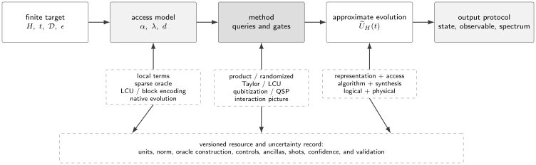
Hamiltonian simulation is a chain of typed interfaces. Complexity statements refer to a particular access box and normalization; scientific accuracy refers to the final observable after representation, algorithm, implementation, and measurement errors have been propagated.

Simulation is not diagonalization

Implementing $e^{-iHt/\hbar}$ does not automatically provide:

• the eigenvalues or eigenvectors of $H$;
• a ground or thermal state;
• all amplitudes of the evolved state;
• a classical description of $H$ learned from data;
• every observable at time $t$;
• an efficient solution for arbitrarily long time.

These may be separate tasks that use Hamiltonian simulation. For example, Quantum Phase Estimation combines controlled evolution with an input having eigenstate overlap and a measurement decoder. Ground-state preparation remains an additional bottleneck. Hamiltonian learning reverses the direction of inference: it uses experimental data to estimate a generator rather than assuming coherent access to that generator.

Metrics and Observable Guarantees

The norm should match the downstream use. Operator norm is convenient for a coherent unitary primitive because it composes under multiplication. If

$$\left\| \widetilde U-U \right\|_{\mathrm{op}} \le\epsilon,$$

then for any normalized $\lvert\psi\rangle$,

$$\left\| \widetilde U\lvert\psi\rangle -U\lvert\psi\rangle \right\| \le\epsilon.$$

The trace distance between the two output pure states is no larger than this vector distance. By convexity, the same state-distance conclusion extends to mixed inputs under the corresponding unitary channels. Consequently, every bounded observable $O$ satisfies

$$\left| \operatorname{Tr} \left[ O \left( \widetilde U\rho\widetilde U^\dagger -U\rho U^\dagger \right) \right] \right| \le 2\lVert O\rVert_\infty\epsilon.$$

This is a worst-case conversion. It may be far looser than the actual error for a local observable, symmetry sector, or selected state. An observable-specific estimate is valuable when it is proved or validated, not when it is inferred merely because the observable is simple.

Errors compose by telescoping

Suppose an algorithm is a product of ideal unitary blocks $U_m\cdots U_1$, while the implementation uses $\widetilde U_m\cdots\widetilde U_1$. Unitary invariance and a telescoping sum give

$$\left\| \widetilde U_m\cdots\widetilde U_1 -U_m\cdots U_1 \right\|_{\mathrm{op}} \le \sum_{j=1}^{m} \left\| \widetilde U_j-U_j \right\|_{\mathrm{op}}.$$

The bound is conservative: coherent errors may cancel or align, and stochastic errors follow a different channel composition. It nevertheless supports an auditable error allocation. Each oracle, arithmetic routine, synthesized rotation, and logical block needs a tolerance compatible with the final budget.

Representation and Hamiltonian Error

Before choosing an algorithm, distinguish the intended Hamiltonian $H$ from the represented generator $\widetilde H$. Duhamel’s identity gives

$$\begin{aligned} e^{-iHt/\hbar} -e^{-i\widetilde Ht/\hbar} &= -\frac{i}{\hbar} \int_0^t e^{-iH(t-s)/\hbar} (H-\widetilde H) e^{-i\widetilde Hs/\hbar} \,ds. \end{aligned}$$

For bounded Hermitian operators,

$$\left\| e^{-iHt/\hbar} -e^{-i\widetilde Ht/\hbar} \right\|_{\mathrm{op}} \le \frac{|t|}{\hbar} \left\| H-\widetilde H \right\|_{\mathrm{op}}.$$

This simple bound has an important consequence: long-time prediction requires correspondingly tighter knowledge of the generator unless structure supplies a better observable-specific argument. More algorithmic precision cannot repair incorrect coefficients, a wrong encoding sector, or a poor physical model.

Energy offsets

For any real $c$,

$$e^{-i(H-cI)t/\hbar} = e^{ict/\hbar} e^{-iHt/\hbar}.$$

The two operators induce the same standalone quantum channel. Subtracting a known energy reference can therefore reduce an LCU or block-encoding normalization without changing state dynamics. The offset is not disposable when the evolution is controlled: its global phase becomes a relative phase on the control. In phase estimation it shifts every inferred energy by $c$ and must be restored in the classical interpretation.

Continuous variables and infinite Hilbert spaces

Circuit algorithms act on finite registers. Bosonic modes, particles in continuum space, and quantum fields therefore require a discretization or cutoff. A declaration such as

$$H_\Lambda = P_\Lambda H P_\Lambda$$

is not yet an error bound. One must control the initial weight outside $P_\Lambda$, transitions through the cutoff boundary, discretization of derivatives or fields, and the target observable’s sensitivity. For unbounded operators, $\lVert H-H_\Lambda\rVert_{\mathrm{op}}$ may be infinite even when low-energy dynamics converge well. State- or energy-constrained estimates are then the appropriate language.

Cutoff size, lattice spacing, volume, boundary conditions, and continuum extrapolation are scientific resources. They should not be hidden inside the qubit count.

Access Models

An access model is a coherent data structure for $H$. Writing down an $N\times N$ matrix classically does not imply an efficient circuit for it. The same mathematical operator can lead to very different simulation costs under different access assumptions.

Exponentiable local terms

Suppose

$$H = \sum_{\ell=1}^{L}H_\ell$$

and each short evolution $e^{-iH_\ell s/\hbar}$ has an efficient circuit. This is the natural input to product formulas and many randomized methods. The contract must include:

• the decomposition and term order;
• the gate cost and error for each exponential;
• term supports and commutation relations;
• whether negative and controlled times are available;
• coefficient precision and update cost.

A decomposition with small $L$ can still be poor if individual exponentials are expensive. A decomposition with large $L$ can be excellent when terms commute in groups, have low-weight Pauli implementations, or admit parallel execution.

Pauli sums and linear combinations of unitaries

For a qubit Hamiltonian

$$H = \sum_{\ell=0}^{L-1} h_\ell P_\ell, \qquad h_\ell\in\mathbb R,$$

define

$$\lambda = \sum_{\ell=0}^{L-1}|h_\ell|.$$

Two coherent oracles provide a standard linear-combination-of-unitaries (LCU) interface. A preparation oracle creates

$$\operatorname{PREPARE}\lvert0\rangle = \sum_{\ell=0}^{L-1} \sqrt{\frac{|h_\ell|}{\lambda}} \lvert\ell\rangle,$$

while

$$\operatorname{SELECT} = \sum_{\ell=0}^{L-1} \lvert\ell\rangle\langle\ell\rvert \otimes \operatorname{sgn}(h_\ell)P_\ell.$$

Their sandwich is

$$\begin{aligned} &\left( \langle0\rvert\operatorname{PREPARE}^\dagger \otimes I \right) \operatorname{SELECT} \left( \operatorname{PREPARE}\lvert0\rangle \otimes I \right) \\ &\qquad = \frac{H}{\lambda}. \end{aligned}$$

Thus the oracle pair block-encodes $H$ with normalization $\lambda$. This identity does not say that PREPARE and SELECT are cheap. Their reversible data lookup, coefficient rotations, Pauli addressing, uncomputation, controls, and fault-tolerant synthesis can dominate the final gate count.

Sparse-matrix oracles

A $d$-sparse Hamiltonian has at most $d$ nonzero entries in each row. A common black-box model provides a location oracle

$$O_F \lvert j,\ell\rangle = \lvert j,f(j,\ell)\rangle$$

for the column of the $\ell$th nonzero entry in row $j$, and a value oracle

$$O_H \lvert j,k,0\rangle = \lvert j,k,H_{jk}\rangle.$$

The arithmetic encoding and precision of $H_{jk}$ are part of the oracle definition. Sparse-oracle simulation bounds commonly depend on a scale such as

$$\alpha_{\mathrm{sparse}} \sim d\lVert H\rVert_{\max},$$

where $\lVert H\rVert_{\max}=\max_{jk}|H_{jk}|$. Query complexity counts calls to $O_F$ and $O_H$; gate complexity must expand those calls into an actual data structure or reversible computation.

Block encoding

With $a$ ancillas, a unitary $U_H$ is an approximate block encoding when

$$\left\| H -\alpha \left( \langle0^a\rvert\otimes I \right) U_H \left( \lvert0^a\rangle\otimes I \right) \right\|_{\mathrm{op}} \le \delta_{\mathrm{BE}}.$$

$\alpha$ and $\delta_{\mathrm{BE}}$ have units of energy in this convention. The normalization obeys $\alpha\gtrsim\lVert H\rVert_{\mathrm{op}}$ and often exceeds it substantially. The natural dimensionless action is

$$\tau = \frac{\alpha|t|}{\hbar}.$$

For fixed oracle cost, larger $\alpha$ makes simulation harder. Quoting a query count without $\alpha$ is therefore incomplete. The block-encoding error alone contributes at most

$$\epsilon_{\mathrm{BE,dyn}} \le \frac{|t|}{\hbar} \delta_{\mathrm{BE}}$$

to a bounded-generator unitary error before any phase-processing error is added.

Native physical access

If a device evolves directly under $H_{\mathrm{lab}}$, physical time itself is an access primitive. This can be efficient, but it changes the verification problem. The generator must be calibrated, unwanted terms bounded, controls modeled, and target time rescaled. Analog Quantum Simulation owns that correspondence. A calibrated native block can also be composed with gates as described on Hybrid Quantum Simulation.

Method Families

No method is best independently of the access model, error target, structure, and hardware cost.

Method	Required access	Governing structure	Principal qualification
deterministic product formulas	exponentials of terms $H_\ell$	nested commutators, locality, ordering, step count	direct and ancilla-light, but precision may require many term exponentials
randomized formulas	sampled term exponentials or Pauli rotations	LCU one-norm and average-channel error	low setup and no coherent index register, but random seeds and channel variance matter
truncated Taylor or LCU	coherent PREPARE and SELECT	coefficient normalization, segment count, series order	strong precision scaling with ancillas, arithmetic, and amplification overhead
qubitization and QSP	controlled block encoding and inverse	$\alpha	t
interaction-picture or Dyson methods	easy evolution under one part plus time-dependent access to another	integrated interaction normalization and time dependence	can remove a large easy term from the main normalization
variational state propagation	parameterized state and measured tangent data	ansatz residual, metric conditioning, shots	state-specific rather than a uniform coherent unitary guarantee
native analog evolution	calibrated physical generator	model mismatch, leakage, physical time	avoids gate decomposition but has no generic symbolic error parameter

Product formulas

For $H=\sum_\ell H_\ell$, product formulas approximate the exponential by a sequence of term evolutions. A coarse first-order error has the form

$$\left\| e^{-iHt/\hbar} -S_1(t/r)^r \right\|_{\mathrm{op}} \lesssim \frac{t^2}{2r\hbar^2} \sum_{j<k} \left\| [H_j,H_k] \right\|,$$

subject to boundedness and higher-order terms. Modern analyses can exploit nested commutators, geometry, conservation laws, and local-observable light cones, producing far tighter bounds than replacing every term by its norm.

The formal order does not determine practical performance. One must include the number of exponentials per step, cancellation, ordering, synthesis precision, connectivity, and physical errors. The full derivation and higher-order recursion are canonical on Trotter Product Formula.

Randomized formulas

For an LCU $H=\sum_\ell h_\ell P_\ell$, qDRIFT samples term $\ell$ with

$$p_\ell = \frac{|h_\ell|}{\lambda}$$

and applies, for each of $N$ samples,

$$V_\ell = \exp\!\left[ -i\,\operatorname{sgn}(h_\ell) \frac{\lambda t}{N\hbar} P_\ell \right].$$

In the basic analysis, the average-channel error scales as

$$\epsilon_{\mathrm{qD}} = O\!\left( \frac{1}{N} \left( \frac{\lambda t}{\hbar} \right)^2 \right).$$

This dependence is independent of the explicit number of terms $L$, which can be attractive when $L$ is large and $\lambda$ remains manageable. The output of one sampled circuit is not the average channel. A reproducible estimate records random seeds, the number of independently sampled sequences, and the variance across them. Hardware noise can interact with sequence randomness rather than merely add to it.

Truncated Taylor and LCU methods

On a short segment $\Delta t$, the Taylor approximation is

$$e^{-iH\Delta t/\hbar} \approx \sum_{k=0}^{K} \frac{1}{k!} \left( -\frac{iH\Delta t}{\hbar} \right)^k.$$

If $x=\lVert H\rVert\,|\Delta t|/\hbar$, the operator-norm tail is bounded by

$$\left\| e^{-iH\Delta t/\hbar} - \sum_{k=0}^{K} \frac{(-iH\Delta t/\hbar)^k}{k!} \right\| \le e^x \frac{x^{K+1}}{(K+1)!}.$$

When $H$ is an LCU, powers $H^k$ become coherent sums of products of the underlying unitaries. Segmenting time keeps coefficient normalization under control; oblivious amplitude amplification converts the desired encoded block into a near-deterministic unitary. The favorable precision dependence is paid for with coefficient-state preparation, SELECT calls, ancillas, reversible arithmetic, and amplification.

Qubitization and quantum signal processing

Given a block encoding of $H/\alpha$, qubitization constructs invariant two-dimensional signal subspaces labeled by eigenvalues

$$x_j = \frac{E_j}{\alpha} \in[-1,1].$$

Quantum signal processing then approximates the eigenvalue function

$$f(x) = e^{-i\tau x}, \qquad \tau=\frac{\alpha t}{\hbar},$$

with a bounded polynomial implemented through repeated signal-oracle calls and single-qubit phase rotations. A robust summary is that the required degree is

$$d = O\!\left( \tau+\log\frac{1}{\epsilon} \right),$$

with sharper query-optimal precision dependence available under standard oracle conventions and asymptotic regimes. For sparse Hamiltonians, quantum signal processing can attain the characteristic bound

$$O\!\left( d_{\mathrm{sparse}} \lVert H\rVert_{\max} \frac{|t|}{\hbar} + \frac{ \log(1/\epsilon) }{ \log\log(1/\epsilon) } \right)$$

in the query model covered by the corresponding theorem.

These are oracle calls, not elementary gates. QSP phase synthesis, controlled block encodings, PREPARE, SELECT, arithmetic, and routing must be costed. The Qubitization and Quantum Signal Processing owns the signal-subspace construction, polynomial admissibility, phase conventions, approximation bounds, validation tests, and fault-tolerant resource expansion.

Interaction-picture simulation

Suppose

$$H=A+B,$$

where evolution under $A$ is easy although $\lVert A\rVert$ is large. Write

$$U_H(t) = e^{-iAt/\hbar}U_I(t),$$

where

$$U_I(t) = \mathcal T \exp\!\left[ -\frac{i}{\hbar} \int_0^t B_I(s)\,ds \right]$$

and

$$B_I(s) = e^{iAs/\hbar} B e^{-iAs/\hbar}.$$

Unitary conjugation preserves $\lVert B_I(s)\rVert$, so a method whose main action depends on $B$ rather than $A+B$ can gain substantially. The gain is conditional: implementing coherent, time-dependent access to $B_I(s)$ may require calls to $e^{\pm iAs/\hbar}$, additional clocks, and more arithmetic. The interaction picture moves complexity; it does not erase it.

Variational and learned surrogates

A parameterized circuit can approximate the action of $U_H(t)$ on a selected state family, or compress a trajectory into a low-dimensional manifold. Such methods can reduce coherent depth but generally do not provide a uniform operator-norm approximation on all inputs. Training data, generalization in time or state, optimization cost, and held-out validation become part of the contract. Hybrid Quantum Simulation owns variational tangent projection and feedback-error propagation.

Generic Limits and Special Structure

Hamiltonian simulation is efficient for broad structured input models, but the evolution time cannot generally be removed from the complexity. There are sparse black-box Hamiltonian families for which simulating time $t$ requires

$$\Omega\!\left( \frac{\alpha|t|}{\hbar} \right)$$

queries in the relevant natural normalization. This no-fast-forwarding statement is a worst-case oracle lower bound. It does not say that every physical Hamiltonian is hard or that every circuit must literally have depth proportional to $t$ under every parallel architecture.

Special Hamiltonians may be fast-forwarded or otherwise simplified because they are diagonal in an efficiently accessible basis, commuting, free, integrable, stabilizer-like, low rank, or restricted to a promised subspace. A classical diagonalization that is exponential in system size is not an efficient fast-forwarding construction. The basis transform, eigenvalue arithmetic, controls, and input promise must all be efficient.

Low-energy and local-observable promises

Worst-case operator-norm simulation treats every input state and every part of the spectrum as relevant. Scientific tasks often impose more structure. An initial state may lie in a low-energy subspace, or the output may be a local observable after finite time. Gap amplification, frustration-free structure, and energy-constrained access can improve some low-energy costs. Lieb–Robinson bounds can restrict the region influencing a local observable and make its cost depend on a spacetime light cone rather than the entire lattice.

These gains require explicit promises. A low expectation value does not imply zero high-energy tail, and power-law interactions can broaden light cones. State leakage, boundary truncation, and the actual observable support must be included in the error statement.

Time-Dependent Hamiltonians

For $H(s)$, the target propagator is

$$U(T,0) = \mathcal T \exp\!\left[ -\frac{i}{\hbar} \int_0^T H(s)\,ds \right].$$

Replacing this expression by $e^{-iT H(T/2)/\hbar}$ is an approximation whose validity depends on time variation and commutators at different times. A time-dependent access contract must state:

• how a coherent time register selects $H(s)$;
• time and coefficient precision;
• continuity, differentiability, or bounded-variation assumptions;
• the cost of querying at one time;
• whether the normalization $\alpha(s)$ is known or sampled;
• how endpoint discontinuities and pulse changes are represented.

Adiabatic Quantum Computation treats a specified gapped Hamiltonian path and schedule as the logical computation model, including endpoint decoding and its own resource normalization. This page retains the distinct task of approximating the resulting time-ordered propagator from a declared access model; native path availability does not automatically supply oracle, block-encoding, controlled, or compiled access.

Under suitable oracle assumptions, time-dependent algorithms can scale with the integrated action

$$\tau_1 = \frac{1}{\hbar} \int_0^T \alpha(s)\,ds$$

rather than the coarser quantity $T\max_s\alpha(s)/\hbar$. This can be a substantial gain for sharply varying or intermittent generators. Dyson-series, time-dependent product-formula, Magnus, rescaling, and interaction-picture methods impose different smoothness and oracle requirements.

If the supplied generator has a time-dependent error $\Delta H(s)$, Duhamel’s argument generalizes to

$$\left\| U_H(T,0) -U_{H+\Delta H}(T,0) \right\| \le \frac{1}{\hbar} \int_0^T \lVert\Delta H(s)\rVert \,ds.$$

This model error is separate from the algorithm’s approximation to the time-ordered exponential.

Worked Example: One Qubit, Three Views

Consider

$$H = aX+bZ, \qquad a,b\in\mathbb R.$$

Let

$$E = \sqrt{a^2+b^2}.$$

Because $(aX+bZ)^2=E^2I$, the exact evolution is

$$U_H(t) = \cos\!\left( \frac{Et}{\hbar} \right)I -i\sin\!\left( \frac{Et}{\hbar} \right) \frac{aX+bZ}{E}.$$

This tiny example separates representation, product-formula error, and LCU normalization.

Product-formula view

A first-order $r$-step circuit is

$$S_r(t) = \left[ e^{-iaXt/(r\hbar)} e^{-ibZt/(r\hbar)} \right]^r.$$

Since

$$[aX,bZ] = -2iabY,$$

the leading coarse global bound scales as

$$\left\| U_H(t)-S_r(t) \right\| \lesssim \frac{|ab|t^2}{r\hbar^2}.$$

The formula is exact when $a=0$ or $b=0$, as the commutator diagnosis predicts. The bound can overestimate the actual periodic error and should not be used as an equality.

LCU and block-encoding view

The Pauli decomposition has

$$\lambda = |a|+|b|.$$

PREPARE uses amplitudes $\sqrt{|a|/\lambda}$ and $\sqrt{|b|/\lambda}$, while SELECT applies the signed $X$ or $Z$. The resulting block encoding has action

$$\tau_{\mathrm{LCU}} = \frac{(|a|+|b|)|t|}{\hbar}.$$

The physical spectral action is $E|t|/\hbar$. Their ratio obeys

$$1 \le \frac{|a|+|b|}{\sqrt{a^2+b^2}} \le \sqrt2.$$

Even here, normalization exceeds the operator norm unless one coefficient vanishes. In large Pauli expansions the gap between an LCU one-norm and the spectral norm can be much larger.

Energy-reference view

If the Hamiltonian were

$$H_c = cI+aX+bZ,$$

including $cI$ in the LCU would raise the naive normalization to $|c|+|a|+|b|$. For state dynamics, simulate $H_c-cI$ and ignore the known global phase. For controlled evolution or energy estimation, apply or account for the phase $e^{-ict/\hbar}$ explicitly. A physically irrelevant offset can be algorithmically expensive if the access model is not centered.

From Evolution to an Observable

The useful output determines which controls, powers, and repetitions are needed.

Schrödinger-picture expectation values

For input $\rho_0$ and observable $O$,

$$\mu_O(t) = \operatorname{Tr} \left[ O U_H(t) \rho_0 U_H^\dagger(t) \right].$$

Estimating $\mu_O$ requires repeated state preparation and measurement. If $O=\sum_j o_jP_j$, shot allocation, grouping, readout calibration, and covariance can dominate the evolution circuit. Hamiltonian simulation does not remove the standard error of sampling.

Correlation functions

A dynamical correlator may be

$$C_{AB}(t) = \langle\psi\rvert U_H^\dagger(t) A U_H(t) B \lvert\psi\rangle.$$

Depending on $A$ and $B$, extracting its real and imaginary parts may require an ancilla interferometer, controlled insertions, backward evolution, or special basis measurements. A circuit that implements only uncontrolled $U_H(t)$ may not satisfy this output contract.

Spectral estimation

If

$$H\lvert E_j\rangle = E_j\lvert E_j\rangle,$$

then

$$U_H(t_0)\lvert E_j\rangle = e^{-iE_jt_0/\hbar} \lvert E_j\rangle.$$

Phase estimation reads $E_jt_0/\hbar$ modulo $2\pi$. Avoiding aliasing requires a known energy interval or multiple-time strategy. Resolving an energy scale $\Delta E$ requires coherent interrogation times of order at least $\hbar/\Delta E$, along with input overlap and controlled simulation. The highest requested precision can therefore set the longest physical or logical evolution even when one short-time oracle call is cheap.

Prepared quantum states

Sometimes the output is the evolved state itself for use by another quantum routine. No immediate tomography is required, but validation still needs operational tests such as symmetries, conserved quantities, Loschmidt echoes, cross-method checks, or selected observables. Saying that a state “is available” should include its preparation success probability and whether the consumer needs a coherent inverse or controlled version.

Error Budget

A simulation-facing error ledger separates at least:

$$\begin{aligned} \epsilon_{\mathrm{total}} \lesssim{}& \epsilon_{\mathrm{model}} +\epsilon_{\mathrm{trunc}} +\epsilon_{\mathrm{encode}} +\epsilon_{\mathrm{access}} \\ &+ \epsilon_{\mathrm{algorithm}} +\epsilon_{\mathrm{synthesis}} +\epsilon_{\mathrm{logical}} +\epsilon_{\mathrm{SPAM}}. \end{aligned}$$

The entries refer to different comparisons:

• model: the chosen Hamiltonian versus the physical system of interest;
• truncation: continuum, bosonic, field, active-space, or volume cutoff;
• encoding: mapping the finite target degrees of freedom into registers;
• access: coefficient error and imperfect PREPARE, SELECT, sparse, or native oracles;
• algorithm: product, randomization, series, or polynomial approximation;
• synthesis: finite-precision rotations and reversible arithmetic;
• logical or physical: faults, decoherence, crosstalk, leakage, and retries;
• SPAM: input preparation and final measurement or estimator error.

The displayed sum is a budgeting device, not a claim of statistical independence. Systematic biases may align, while stochastic uncertainties should be propagated with covariance. Error mitigation can trade bias for variance and does not remove model or algorithmic error.

Allocate error to the output

Suppose the final goal is an observable tolerance $\epsilon_O$. If a trace- distance budget $D_{\mathrm{dyn}}$ is assigned to preparation and dynamics, then

$$\epsilon_O \ge 2\lVert O\rVert_\infty D_{\mathrm{dyn}} +\epsilon_{\mathrm{meas}}$$

is a conservative allocation. A solver should not automatically drive its unitary approximation to machine precision when model uncertainty or shot noise is much larger. Conversely, a loose unitary tolerance can be unacceptable for a small signal produced by cancellation between large terms.

Resource Accounting

Query complexity is one line in a complete ledger. For a block-encoding method, report:

1. number of calls to $U_H$, $U_H^\dagger$, and controlled variants;
2. gate and depth cost of PREPARE, SELECT, sparse lookup, or arithmetic;
3. block-encoding normalization $\alpha$ and approximation $\delta_{\mathrm{BE}}$;
4. QSP or LCU ancillas, phase precision, and amplification;
5. logical one- and two-qubit gates, non-Clifford gates, and routing;
6. code cycles, logical failure budget, and physical qubits if fault tolerant;
7. state preparations, accepted postselections, measurements, and retries;
8. classical preprocessing, coefficient generation, compilation, and phase synthesis;
9. maximum coherent depth, total interrogation time, and wall-clock latency;
10. output-estimation cost at the requested confidence.

If one block-encoding query costs $G_{\mathrm{BE}}$ logical gates and the phase-processing sequence makes $Q$ queries, a first expansion is

$$G_{\mathrm{signal}} \approx QG_{\mathrm{BE}} +G_{\mathrm{phases}} +G_{\mathrm{control}}.$$

This is still not a hardware estimate. Routing, error correction, measurement, and repetition remain. Resource Estimation Tools owns the conversion from logical artifacts to architecture-dependent costs.

Compare equivalent access

A quantum sparse-oracle algorithm should be compared with a classical method given equivalent sparse access, not with a classical program forced to scan a dense matrix. An LCU query should not be priced as one gate if PREPARE performs a large data lookup. Likewise, a classical tensor-network or Monte Carlo method may exploit locality, low entanglement, a favorable sign structure, or a restricted observable that a worst-case Hilbert-space argument ignores.

An end-to-end advantage claim specifies the same model, state family, observable, time, error, confidence, and input-access assumptions on both sides.

Validation

Hamiltonian simulation has three distinct validation layers.

Access validation

Check that the implemented oracle represents the intended operator:

• reconstruct small PREPARE and SELECT instances;
• verify Hermiticity, coefficient signs, basis ordering, and units;
• compare block-encoding matrix elements on sampled states;
• test sparse lookup reversibility and duplicate-entry conventions;
• quantify arithmetic and coefficient quantization;
• characterize native generators over the claimed control region.

Algorithm validation

On classically tractable sizes:

• compare full unitaries up to the correct global-phase convention;
• test multiple input states and held-out observables;
• vary product-formula step count, Taylor order, QSP degree, or random samples;
• verify predicted precision scaling rather than one operating point;
• test commuting, zero-coupling, short-time, and symmetry limits;
• separate series or polynomial error from oracle approximation.

End-to-end validation

For the scientific task:

• include state preparation and readout;
• check conservation laws and positivity constraints;
• compare local observables in overlapping classical regimes;
• propagate model and calibration uncertainty;
• reserve data not used to tune the circuit or stopping rule;
• report failed runs, postselection, mitigation, and branch choices;
• compare total resources at matched accuracy.

A small circuit-level distance on a toy instance is component evidence. It is not a material prediction or a quantum-advantage demonstration by itself.

Choosing a Method

A practical decision sequence is:

1. Fix the output. Is the task a state, local observable, correlation, sample, or eigenphase?
2. Fix the domain and metric. Is worst-case operator norm required, or is a state, energy sector, or light cone sufficient?
3. Audit representation error. Set cutoffs and coefficient precision before spending the algorithmic budget.
4. Expose available access. Price term exponentials, PREPARE, SELECT, sparse lookup, block encoding, and controls in the same gate model.
5. Compute structural parameters. Include commutators, locality, $\lambda$, $\alpha$, integrated action, and target time.
6. Compare complete candidates. Expand queries into gates, ancillas, synthesis, logical error, and output measurements.
7. Validate scaling. Use small exact instances and convergence studies before extrapolating.

Product formulas often remain competitive when term evolutions are native, commutators are favorable, ancillas are scarce, or moderate accuracy is enough. Qubitization is compelling when a low-normalization block encoding is already efficient and high precision or long fault-tolerant evolution is required. Randomized methods can be attractive for large Pauli sums with moderate one-norm. Interaction-picture methods help when a large part is easy to evolve. These are conditional judgments, not a universal ranking.

Common Mistakes

Omitting $\hbar$ without declaring units

Algorithm papers often use $\hbar=1$. When laboratory energies and times are inserted, the dimensionless action is $\alpha t/\hbar$. State the convention.

Calling a matrix description an oracle

A classical table is not automatically a coherent, reversible lookup. Specify data loading, arithmetic precision, controls, inverse access, and gate cost.

Comparing query counts with gate counts

One PREPARE or SELECT query may contain many logical gates and memory accesses. Expand the oracle before claiming a hardware advantage.

Hiding normalization

The block-encoding scale $\alpha$ or LCU one-norm $\lambda$ multiplies time in the central complexity parameter. A low query count with a poor normalization can be worse than a direct formula.

Treating a global phase inconsistently

Energy shifts are harmless for standalone state dynamics but observable in a controlled branch and essential for energy interpretation.

Using product-formula order as a performance prediction

Formal order omits commutator constants, number of exponentials, cancellation, and hardware error. Benchmark the complete circuit at the target regime.

Calling one random sequence the average channel

Randomized simulation guarantees often concern expectation over compiler seeds. Report seed variation and the sampling protocol.

Forgetting truncation in bosonic or field models

The finite qubit Hamiltonian is already an approximation. Cutoff leakage and continuum extrapolation can dominate gate-synthesis error.

Equating evolution with readable output

Correlation functions may need controls and reverse evolution; spectra need long interrogation and input overlap; observables need shots. Count them.

Applying no-fast-forwarding to every Hamiltonian

It is a worst-case oracle result. Commuting, integrable, free, diagonal, and promised-subspace families may admit faster constructions.

Research Status

Efficient Hamiltonian simulation under local-term, sparse-oracle, LCU, and block-encoding access is established. Product formulas have rigorous commutator- and locality-aware analyses; truncated-series methods give strong precision dependence; qubitization and quantum signal processing achieve near-optimal or optimal query scaling in standard black-box models. Generic no-fast-forwarding lower bounds explain why linear dependence on normalized time is unavoidable in the worst case.

As of 2026, active work concerns practically tighter commutator bounds, multi-product and hybrid formulas, time-dependent and unbounded generators, low-energy and local-observable promises, parallel depth, oracle implementation, and fault-tolerant resource reduction. Improvements in query complexity do not automatically improve logical gate count. For concrete chemistry, materials, and field-theory problems, representation choice and data-access circuits remain central engineering and scientific questions.

Key Results

• Hamiltonian simulation implements a quantum evolution primitive; it does not by itself diagonalize $H$, prepare an eigenstate, or return a wavefunction.
• The input includes a coherent access model. Local terms, sparse oracles, LCU data, block encodings, and native dynamics are not interchangeable.
• For a block encoding with energy normalization $\alpha$, the central action is $\tau=\alpha|t|/\hbar$; oracle error and Hamiltonian error grow at most linearly with time in a basic Duhamel bound.
• Product formulas exploit commutators and locality; randomized formulas trade coherent ordering for average-channel error; LCU and QSP methods exchange more elaborate access for strong precision scaling.
• Generic black-box Hamiltonians cannot be fast-forwarded, but explicit structure or state and observable promises can reduce cost.
• Controlled evolution, correlation functions, phase estimation, and local observables impose different output interfaces and resource requirements.
• Trustworthy claims propagate representation, access, algorithm, synthesis, hardware, and measurement errors to the declared observable.

References

1. R. P. Feynman, “Simulating physics with computers,” International Journal of Theoretical Physics 21, 467–488 (1982), doi:10.1007/BF02650179.
2. S. Lloyd, “Universal quantum simulators,” Science 273, 1073–1078 (1996), doi:10.1126/science.273.5278.1073.
3. D. W. Berry, G. Ahokas, R. Cleve, and B. C. Sanders, “Efficient quantum algorithms for simulating sparse Hamiltonians,” Communications in Mathematical Physics 270, 359–371 (2007), doi:10.1007/s00220-006-0150-x.
4. A. M. Childs and N. Wiebe, “Hamiltonian simulation using linear combinations of unitary operations,” Quantum Information and Computation 12, 901–924 (2012), arXiv:1202.5822.
5. D. W. Berry, A. M. Childs, R. Cleve, R. Kothari, and R. D. Somma, “Simulating Hamiltonian dynamics with a truncated Taylor series,” Physical Review Letters 114, 090502 (2015), doi:10.1103/PhysRevLett.114.090502.
6. D. W. Berry, A. M. Childs, and R. Kothari, “Hamiltonian simulation with nearly optimal dependence on all parameters,” in 2015 IEEE 56th Annual Symposium on Foundations of Computer Science, 792–809 (2015), doi:10.1109/FOCS.2015.54.
7. G. H. Low and I. L. Chuang, “Optimal Hamiltonian simulation by quantum signal processing,” Physical Review Letters 118, 010501 (2017), doi:10.1103/PhysRevLett.118.010501.
8. G. H. Low and I. L. Chuang, “Hamiltonian simulation by qubitization,” Quantum 3, 163 (2019), doi:10.22331/q-2019-07-12-163.
9. A. Gilyén, Y. Su, G. H. Low, and N. Wiebe, “Quantum singular value transformation and beyond: exponential improvements for quantum matrix arithmetics,” in Proceedings of the 51st Annual ACM SIGACT Symposium on Theory of Computing, 193–204 (2019), doi:10.1145/3313276.3316366.
10. E. Campbell, “Random compiler for fast Hamiltonian simulation,” Physical Review Letters 123, 070503 (2019), doi:10.1103/PhysRevLett.123.070503.
11. A. M. Childs, Y. Su, M. C. Tran, N. Wiebe, and S. Zhu, “Theory of Trotter error with commutator scaling,” Physical Review X 11, 011020 (2021), doi:10.1103/PhysRevX.11.011020.
12. A. M. Childs and Y. Su, “Nearly optimal lattice simulation by product formulas,” Physical Review Letters 123, 050503 (2019), doi:10.1103/PhysRevLett.123.050503.
13. A. M. Childs, D. Maslov, Y. Nam, N. J. Ross, and Y. Su, “Toward the first quantum simulation with quantum speedup,” Proceedings of the National Academy of Sciences 115, 9456–9461 (2018), doi:10.1073/pnas.1801723115.
14. D. W. Berry, A. M. Childs, Y. Su, X. Wang, and N. Wiebe, “Time-dependent Hamiltonian simulation with $L^1$-norm scaling,” Quantum 4, 254 (2020), doi:10.22331/q-2020-04-20-254.
15. G. H. Low and N. Wiebe, “Hamiltonian simulation in the interaction picture,” arXiv:1805.00675 (2018), doi:10.48550/arXiv.1805.00675.
16. J. Haah, M. B. Hastings, R. Kothari, and G. H. Low, “Quantum algorithm for simulating real time evolution of lattice Hamiltonians,” in 2018 IEEE 59th Annual Symposium on Foundations of Computer Science, 350–360 (2018), doi:10.1109/FOCS.2018.00041.
17. Y. Atia and D. Aharonov, “Fast-forwarding of Hamiltonians and exponentially precise measurements,” Nature Communications 8, 1572 (2017), doi:10.1038/s41467-017-01637-7.
18. D. Poulin, A. Qarry, R. D. Somma, and F. Verstraete, “Quantum simulation of time-dependent Hamiltonians and the convenient illusion of Hilbert space,” Physical Review Letters 106, 170501 (2011), doi:10.1103/PhysRevLett.106.170501.
19. I. D. Kivlichan et al., “Improved fault-tolerant quantum simulation of condensed-phase correlated electrons via Trotterization,” Quantum 4, 296 (2020), doi:10.22331/q-2020-07-16-296.
20. A. Zlokapa and R. D. Somma, “Hamiltonian simulation for low-energy states with optimal time dependence,” Quantum 8, 1449 (2024), doi:10.22331/q-2024-08-27-1449.
21. I. M. Georgescu, S. Ashhab, and F. Nori, “Quantum simulation,” Reviews of Modern Physics 86, 153–185 (2014), doi:10.1103/RevModPhys.86.153.
22. S. McArdle et al., “Quantum computational chemistry,” Reviews of Modern Physics 92, 015003 (2020), doi:10.1103/RevModPhys.92.015003.

Further Connections

• Algorithmic Primitives introduces block encoding, QSP, phase estimation, amplification, and postselection as reusable interfaces.
• Digital Quantum Simulation carries the primitive through representation, state preparation, compilation, hardware execution, measurement, and validation.
• Qubitization and Quantum Signal Processing develops block encodings, invariant signal planes, QSP polynomials and phases, spectral readout, and oracle-level resource accounting.
• Simulation of Quantum Chemistry shows how molecular representation, integral factorization, state preparation, and the requested chemical output instantiate a Hamiltonian-simulation contract.
• Simulation of Quantum Materials shows how periodic and effective-model representations, finite cells, preparation, spectra, response, and thermodynamic workflows instantiate that contract for materials.
• Trotter–Suzuki Methods develops executable decompositions, commutator-sensitive error and lattice scaling, ordering, compilation, and convergence tests.
• Trotter Product Formula derives first-, second-, and higher-order splitting formulas and their mathematical hypotheses.
• Quantum Phase Estimation explains eigenstate overlap, controlled powers, phase statistics, aliasing, and energy resolution.
• Hybrid Quantum Simulation covers native analog blocks, variational projected dynamics, embedding, and feedback loops.
• Analog Quantum Simulation treats physical generator correspondence, time rescaling, leakage, and observable-level validation.
• Algorithmic Benchmarking defines task-level quality and matched end-to-end resource comparison.
• Noise in Quantum Information distinguishes coherent, stochastic, leakage, drift, and mitigation effects from ideal algorithmic error.

Exercises

1. Convert unitary error to observable error

Let $\lVert\widetilde U-U\rVert_{\mathrm{op}}\le\epsilon$. Show that for every normalized pure input and bounded observable $O$, the expectation values after the two evolutions differ by at most $2\lVert O\rVert_\infty\epsilon$.

Solution

Define

$$\lvert\phi\rangle =U\lvert\psi\rangle, \qquad \lvert\widetilde\phi\rangle =\widetilde U\lvert\psi\rangle.$$

Then

$$\lVert\widetilde\phi-\phi\rVert \le \lVert\widetilde U-U\rVert_{\mathrm{op}} \le\epsilon.$$

Add and subtract $\langle\widetilde\phi\rvert O\lvert\phi\rangle$:

$$\begin{aligned} &\left| \langle\widetilde\phi\rvert O\lvert\widetilde\phi\rangle -\langle\phi\rvert O\lvert\phi\rangle \right| \\ &\quad\le \left| \langle\widetilde\phi\rvert O (\lvert\widetilde\phi\rangle-\lvert\phi\rangle) \right| \\ &\qquad+ \left| (\langle\widetilde\phi\rvert-\langle\phi\rvert) O \lvert\phi\rangle \right| \\ &\quad\le 2\lVert O\rVert_\infty\epsilon. \end{aligned}$$

The result is worst-case and may be loose for a particular state and observable.

2. Center an energy interval

Suppose the spectrum of $H$ lies in $[E_{\min},E_{\max}]$. Choose a scalar $c$ that minimizes $\lVert H-cI\rVert_{\mathrm{op}}$ and give the minimum. Why must $c$ still be recorded for phase estimation?

Solution

For Hermitian $H$,

$$\lVert H-cI\rVert_{\mathrm{op}} = \max \left( |E_{\min}-c|, |E_{\max}-c| \right).$$

The minimax choice is the interval midpoint,

$$c = \frac{E_{\min}+E_{\max}}{2},$$

giving

$$\min_c \lVert H-cI\rVert_{\mathrm{op}} = \frac{E_{\max}-E_{\min}}{2}.$$

The centered Hamiltonian produces the same standalone state dynamics up to a global phase. Phase estimation measures phases relative to the control, so its energies are shifted by $-c$; adding $c$ back is necessary to report the original spectrum.

3. Verify the LCU block encoding

Using the PREPARE and SELECT definitions in the text, prove that their all-zero ancilla block equals $H/\lambda$. What fails if the coefficient signs are omitted from SELECT?

Solution

Let

$$\lvert G\rangle = \sum_\ell \sqrt{\frac{|h_\ell|}{\lambda}} \lvert\ell\rangle.$$

Then

$$\begin{aligned} (\langle G\rvert\otimes I) \operatorname{SELECT} (\lvert G\rangle\otimes I) &= \sum_\ell \frac{|h_\ell|}{\lambda} \operatorname{sgn}(h_\ell)P_\ell \\ &= \frac{1}{\lambda} \sum_\ell h_\ell P_\ell = \frac{H}{\lambda}. \end{aligned}$$

Without the signs, the encoded operator would be $\sum_\ell|h_\ell|P_\ell/\lambda$, generally a different Hamiltonian.

4. Compare the one-qubit actions

For $H=aX+bZ$, evaluate the ratio

$$R = \frac{|a|+|b|}{\sqrt{a^2+b^2}}$$

when $|a|=|b|$ and when $b=0$. Interpret the result.

Solution

If $|a|=|b|\ne0$, then

$$R = \frac{2|a|}{\sqrt2|a|} = \sqrt2.$$

If $b=0$ and $a\ne0$, then $R=1$. The LCU normalization equals the spectral norm for a single Pauli term but exceeds it when noncommuting components are encoded separately. Query complexity responds to the access normalization, not only to the physical spectral scale.

5. Allocate qDRIFT samples

Let $\lambda|t|/\hbar=20$. Using a basic bound $\epsilon_{\mathrm{qD}}\le2(\lambda t/\hbar)^2/N$, how many sampled exponentials are sufficient for error at most $0.01$? What does this number omit?

Solution

The condition is

$$\frac{2(20)^2}{N} \le0.01,$$

so

$$N \ge 80{,}000.$$

This is a sufficient count under the stated average-channel bound. It omits constants from a different theorem convention, variation across random sequences, gate synthesis and hardware noise, the number of sequence samples needed for the final estimator, state preparation, and measurement shots.

6. Prove the Hamiltonian perturbation bound

Use Duhamel’s identity to prove

$$\left\| e^{-iHt/\hbar} -e^{-i\widetilde Ht/\hbar} \right\| \le \frac{|t|}{\hbar} \lVert H-\widetilde H\rVert$$

for bounded Hermitian $H$ and $\widetilde H$.

Solution

For $t\ge0$, define

$$F(s) = e^{-iH(t-s)/\hbar} e^{-i\widetilde Hs/\hbar}.$$

Differentiation and integration from $0$ to $t$ give

$$e^{-i\widetilde Ht/\hbar} -e^{-iHt/\hbar} = \frac{i}{\hbar} \int_0^t e^{-iH(t-s)/\hbar} (H-\widetilde H) e^{-i\widetilde Hs/\hbar} \,ds.$$

Both exponentials are unitary, so submultiplicativity gives

$$\left\| e^{-i\widetilde Ht/\hbar} -e^{-iHt/\hbar} \right\| \le \frac{1}{\hbar} \int_0^t \lVert H-\widetilde H\rVert\,ds.$$

This equals $t\lVert H-\widetilde H\rVert/\hbar$. Reversing time gives the absolute-value form.

7. Compare maximum and integrated normalization

A time-dependent oracle has normalization $\alpha(s)=\alpha_0$ for a fraction $q$ of the interval $[0,T]$ and zero otherwise. Compare $T\max_s\alpha(s)/\hbar$ with the integrated action $\tau_1$.

Solution

The maximum-based quantity is

$$\frac{\alpha_0T}{\hbar}.$$

The integrated action is

$$\tau_1 = \frac{1}{\hbar} \int_0^T\alpha(s)\,ds = \frac{q\alpha_0T}{\hbar}.$$

An algorithm with valid $L^1$-norm scaling can improve the normalization dependence by a factor $1/q$ in this idealized intermittent example. The gain assumes that coherent time access and sampling do not introduce a compensating cost.

8. Audit a spectral-simulation claim

A proposal reports $Q=10^7$ block-encoding queries to estimate an energy at resolution $10^{-3}$, but does not state $\alpha$, PREPARE cost, input overlap, or controlled-query construction. List the missing information needed for an end-to-end assessment.

Solution

At minimum, the assessment needs:

1. energy units, $\hbar$ convention, simulation times, and block normalization $\alpha$;
2. the block-encoding error and coefficient or arithmetic precision;
3. logical gate, depth, ancilla, and non-Clifford cost of PREPARE, SELECT, their inverses, and controlled variants;
4. QSP, LCU, or product-formula approximation and synthesis tolerances;
5. the trial state’s overlap with the desired eigenspace and repetition or amplification cost;
6. aliasing interval, energy offset, phase-estimation failure probability, and total interrogation time;
7. error-correction, routing, logical failure, physical-qubit, and wall-clock assumptions;
8. state-preparation, measurement, retries, classical preprocessing, and a matched classical baseline.

Without these items, $Q$ is an oracle-model statistic rather than an executable resource estimate.