Algorithmic Primitives

Short Definition

An algorithmic primitive is a reusable transformation or access pattern that performs one recognizable part of a quantum algorithm. Typical primitives:

• prepare a structured superposition;
• query data or a function coherently;
• convert eigenvalues or function values into relative phase;
• interfere amplitudes so that useful labels are enhanced or revealed;
• transform spectral information with Fourier or polynomial methods;
• amplify a desired subspace;
• simulate generated dynamics;
• condition on a measurement outcome.

A primitive is not a speedup by itself. A complete algorithm must connect a stated input model to a classically readable output with a success guarantee and a resource bound. The difficult step is often the interface between primitives: preparing the input, implementing controlled access, normalizing an encoded operator, or extracting a useful statistic.

This page is the canonical home for the pattern language and interfaces shared by quantum algorithms. It previews phase kickback, the quantum Fourier transform, phase estimation, amplitude amplification, Hamiltonian simulation, block encoding, quantum signal processing, and postselection. Their full derivations, optimal bounds, and application-specific variants belong to dedicated pages. Circuit Model fixes circuit semantics; Universal Gate Sets fixes synthesis and fault-tolerant gate alphabets.

A Quantum Algorithm Is a Contract

A useful algorithm statement specifies more than a circuit diagram:

Contract item	Questions that must be answered
problem	What mathematical relation or decision problem is being solved?
input model	Classical description, prepared state, sample access, sparse oracle, block encoding, or physical Hamiltonian?
output	Bitstring, sample, expectation value, eigenvalue estimate, or prepared state?
success	Exact, bounded error, approximation tolerance, confidence level, or heralded event?
cost model	Queries, gates, depth, qubits, measurements, classical work, or physical time?
comparison	Which classical access model and algorithm receive the same input information?

Query complexity can be much smaller than gate complexity when an oracle call hides a large computation. A polylogarithmic quantum circuit after state preparation can still have an expensive end-to-end data-loading step. Conversely, a primitive with no asymptotic advantage can remain valuable as part of a larger construction.

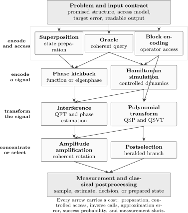
Quantum algorithms compose access, coherent signal processing, concentration, and readout. The same primitive can appear at several layers: Hamiltonian simulation can create the controlled unitary used by phase estimation, while block encoding can supply the signal transformed by quantum signal processing.

Superposition Over Inputs

For $N=2^n$, Hadamard gates prepare the uniform superposition

$$H^{\otimes n}\lvert0^n\rangle = \frac1{\sqrt N} \sum_{x=0}^{N-1} \lvert x\rangle.$$

This state makes coherent access to all basis labels possible. It does not make all classical function values available for simultaneous readout. One computational-basis measurement still returns one $x$, uniformly distributed.

More generally, a state-preparation circuit $\mathcal A$ may produce

$$\mathcal A\lvert0^n\rangle = \sum_x \sqrt{p_x}\,e^{i\theta_x} \lvert x\rangle.$$

The amplitudes define which inputs receive weight and how later paths interfere. Preparing the uniform state is cheap, but preparing an arbitrary amplitude-encoded data vector generally is not. An algorithm that begins with “load the data state” must count the circuit, memory, oracle, or physical process that performs that step.

Quantum Machine Learning owns learning-specific data and feature maps; this page retains the generic access and state-preparation interface.

Superposition becomes useful only when later operations produce structured relative phases or correlations. Probability Amplitudes owns the distinction between amplitudes and observable probabilities.

Oracles and Coherent Access

An oracle specifies how an algorithm accesses a function or data structure. Quantum Oracles owns the complete access record: domains and promises, full-space action, separately supplied forward, inverse, controlled, powered, or family capabilities, licensed reductions between forms, query convention, and oracle-specific fair comparator. This page begins from that declared interface and tracks how it composes with phase, interference, amplification, spectral processing, and readout. For a Boolean function $f$, a common reversible form is

$$O_f \lvert x\rangle\lvert y\rangle = \lvert x\rangle \lvert y\oplus f(x)\rangle.$$

Reversible Computation develops the embedding and cleanup contract behind this oracle form; the access record must distinguish an abstract supplied unitary from a constructed reversible implementation.

Controlled Operations audits the projector/block semantics, branch phase, inverse convention, and license for controlled access; this page composes only the capabilities that the declared interface actually supplies.

Linearity determines its action on superpositions. If the input register is in $\sum_x\alpha_x\lvert x\rangle$, one call creates

$$\sum_x \alpha_x \lvert x\rangle \lvert y\oplus f(x)\rangle.$$

This is coherent evaluation, not a list of readable answers. Measuring generally reveals only one branch and can destroy phase relations among branches.

A phase oracle for a predicate $\chi$ has the form

$$P_\chi\lvert x\rangle = (-1)^{\chi(x)} \lvert x\rangle.$$

Phase oracles are convenient in interference and amplitude amplification. They can often be constructed from reversible evaluation plus an ancilla, but uncomputation and temporary workspace must be included.

An oracle model is an abstraction. A fair complexity claim states:

• what one query returns coherently;
• whether inverse and controlled queries are available;
• the gate cost of a query when it is known;
• whether the classical comparator receives equivalent access.

Oracle separations prove statements about an access model, not automatically about total runtime on explicit data.

Query Complexity begins at this boundary: it owns formal deterministic, randomized, exact, zero-error, and bounded-error query measures, reductions, and lower-bound certificates, while this page retains the procedural composition of licensed primitives.

Phase Kickback

Phase Kickback owns the general common-eigenstate and character-state derivation, the clean Boolean XOR-to-phase and modular-addition conversions, target-return and cleanup tests, and phase-sensitive verification. At the algorithm-interface level, a licensed coherent branch operation can place an eigenvalue or clean function value into a relative phase while its target returns or factors; a later interference step can turn that phase pattern into observable probabilities.

The primitive record must keep controlled or oracle access, ancilla preparation, garbage cleanup, synthesis, interference, and readout as separate obligations. The algebraic phase conversion alone establishes neither an accessible answer nor an algorithmic speedup.

Interference

Interference is the controlled addition of complex amplitudes associated with indistinguishable alternatives. For

$$\lvert\psi\rangle = \sum_x a_x\lvert x\rangle,$$

the Walsh–Hadamard transform produces output amplitude

$$b_y = \frac1{\sqrt N} \sum_x (-1)^{x\cdot y} a_x.$$

The signs can make unwanted amplitudes cancel and useful amplitudes add. Unitarity preserves total probability:

$$\sum_y\lvert b_y\rvert^2 = \sum_x\lvert a_x\rvert^2.$$

An algorithm does not create probability from nothing; it redistributes probability among outcomes by rotating amplitudes. The design problem is to arrange a phase pattern whose Fourier, reflection, or polynomial transform makes the desired property measurable.

Entanglement is neither necessary for every small interference example nor sufficient for a speedup. The operational question is what global structure the circuit extracts with fewer resources under the stated access model.

Deutsch–Jozsa Algorithm is the canonical finite Boolean example of this interference step: a promised sign pattern has a zero-frequency Walsh coefficient of magnitude one when constant and zero when balanced. Its page owns the named promise, exact decision proof, and matched classical query comparison; this page retains the reusable transform vocabulary.

Bernstein–Vazirani Algorithm owns the affine-character recovery theorem for a hidden linear word, including its exact one-query decoding proof and matched $n$-query classical comparison. This page retains the reusable transform language that identifies a character label through interference.

Simon’s Algorithm owns value-oracle coset entanglement, Fourier sampling in an orthogonal subspace, binary-rank recovery and verification, and its matched classical collision bounds. This page retains the reusable access–interference–readout and classical-postprocessing vocabulary.

Quantum Fourier Transform

The Quantum Fourier Transform page owns binary factorization, circuit construction, swap semantics, approximation cutoffs, and verification. At the interface level, the transform on an $N$-dimensional computational basis is

$$F_N\lvert x\rangle = \frac1{\sqrt N} \sum_{k=0}^{N-1} e^{2\pi i xk/N} \lvert k\rangle.$$

For $N=2^n$, the standard circuit uses Hadamard gates and controlled phase rotations, followed by a bit-order reversal. Its exact gate count is quadratic in $n$ for the usual decomposition; omitting sufficiently small rotations gives useful approximate circuits.

The quantum Fourier transform and the classical fast Fourier transform solve different interface problems:

• the classical FFT receives a list of $N$ numbers and returns a list of $N$ Fourier coefficients;
• the QFT transforms amplitudes of a quantum state in time polynomial in $\log N$ but does not print all $N$ output amplitudes.

The QFT is valuable when measurement of the transformed state reveals a compact property such as a period or an eigenphase. It is not a generic exponentially fast replacement for every classical Fourier analysis. Fast Fourier Transform owns the classical algorithm and its data-access model.

Phase Estimation

Let

$$U\lvert u_j\rangle = e^{2\pi i\phi_j} \lvert u_j\rangle, \qquad 0\leq\phi_j<1.$$

Quantum phase estimation uses a control register, controlled powers $U^{2^r}$, phase kickback, and an inverse QFT to estimate $\phi_j$. In the idealized exactly representable case,

$$\lvert0^m\rangle\lvert u_j\rangle \longmapsto \lvert\phi_j\rangle_m \lvert u_j\rangle.$$

For an input superposition of eigenstates,

$$\lvert\psi\rangle = \sum_j c_j\lvert u_j\rangle,$$

the coherent output is

$$\sum_j c_j \lvert\widetilde{\phi_j}\rangle \lvert u_j\rangle.$$

Measuring the estimate register samples eigenphase $j$ with probability approximately $\lvert c_j\rvert^2$, broadened by finite precision. Phase estimation therefore does not find an eigenvalue absent from the input state: overlap with the desired eigenspace is a resource.

The precision ledger must count controlled evolution time. Treating $U^{2^r}$ as one unit-cost gate hides the dominant resource in many physical applications. Standard phase estimation has total controlled-$U$ evolution scaling inversely with target additive phase precision, up to success-probability and implementation details.

Quantum Phase Estimation derives the phase-gradient state, inverse-QFT probability kernel, guard-bit guarantee, energy aliasing rule, iterative variants, and full powered-unitary cost.

Shor Algorithm is the canonical arithmetic composition: structured modular powers make phase estimation efficient, and continued fractions convert sampled eigenphases into a verified multiplicative order.

Amplitude Amplification

Let a state-preparation unitary $\mathcal A$ produce

$$\begin{aligned} \mathcal A\lvert0\rangle &= \sin\theta\,\lvert G\rangle + \cos\theta\,\lvert B\rangle, \\ \sin^2\theta &= a. \end{aligned}$$

where $\lvert G\rangle$ and $\lvert B\rangle$ are normalized states in the good and bad subspaces. One amplitude-amplification iterate composes:

1. a phase reflection on the good subspace;
2. $\mathcal A^\dagger$;
3. a reflection about the initial state;
4. $\mathcal A$.

Up to a convention-dependent global sign, this iterate rotates the two-dimensional good–bad plane by $2\theta$. After $r$ iterations,

$$\begin{aligned} Q^r\mathcal A\lvert0\rangle &= \sin\!\left((2r+1)\theta\right) \lvert G\rangle \\ &\quad+ \cos\!\left((2r+1)\theta\right) \lvert B\rangle. \end{aligned}$$

Classical repetition needs an expected $O(1/a)$ state preparations to observe a good event. Coherent amplitude amplification uses $O(1/\sqrt a)$ calls to $\mathcal A$, $\mathcal A^\dagger$, and the relevant reflections.

This quadratic improvement has conditions. The preparation must remain coherent, its inverse must be available, and the good subspace must be marked. If $a$ is unknown, blindly applying too many iterations rotates probability away from the target; randomized schedules, estimation, or fixed-point variants address that issue.

Grover Search is the canonical worked instance: uniform preparation and a Boolean marking oracle yield an exact two-reflection rotation, a stopping rule, and an optimal $\Theta(\sqrt{N/M})$ query bound.

Amplitude Amplification owns the general arbitrary-preparation theorem, known- and unknown-success schedules, exact and fixed-point regimes, coherent-error budget, and separate accounting of $\mathcal A$, $\mathcal A^\dagger$, both reflections, measurement, and verification.

Amplitude Estimation composes that iterate’s conjugate eigensystem with phase decoding and owns the full estimation ledger across preparation, controlled powers, phase decoding, probability error, confidence, and classical inference.

Hamiltonian Simulation

Hamiltonian simulation asks for a circuit approximating

$$U(t)=e^{-iHt}$$

to a stated error. It turns a description or access procedure for a Hamiltonian into controlled dynamics that other primitives can use.

What Is Quantum Simulation? places this primitive inside the larger scientific workflow: target-model mapping, state preparation, observable extraction, device error, validation, and matched classical baselines.

Hamiltonian Simulation retains the primitive’s simulation-facing task, norm and domain choices, local-term, sparse, LCU, and block-encoding access, time-dependent extensions, finite-dimensional truncation, error and output interfaces, and propagation to measurable outputs. Hamiltonian Simulation Algorithms owns the theorem-level cross-family map of method applicability, normalized upper and lower query bounds, and query-to-resource qualifications.

The complexity depends on the input model. Examples include:

• a sum of local terms with circuits for each term;
• sparse-matrix oracles returning nonzero positions and values;
• a linear combination of efficiently implementable unitaries;
• a block encoding with normalization factor $\alpha$;
• direct analog evolution under a controllable physical Hamiltonian.

Trotter Product Formula owns the operator-splitting derivation. Linear-combination, qubitization, and quantum-signal-processing methods can provide different dependence on time, precision, and access parameters.

Simulating $e^{-iHt}$ is not the same as learning the full evolved wavefunction. Useful applications specify a prepared input and a measurable output: a correlation function, eigenphase sample, transition amplitude, or local observable. State preparation and measurement repetitions can dominate.

Block Encoding

A block encoding represents a possibly nonunitary operator $A$ as a sub-block of a larger unitary $U_A$. With $a$ ancilla qubits, define

$$B = \left( \langle0^a\rvert\otimes I \right) U_A \left( \lvert0^a\rangle\otimes I \right).$$

The unitary is an $(\alpha,a,\epsilon)$ block encoding when

$$\left\| A-\alpha B \right\|_{\mathrm{op}} \leq \epsilon.$$

The normalization $\alpha$ is algorithmically important. In the exact case, applying $U_A$ to $\lvert0^a\rangle\lvert\psi\rangle$ and projecting the ancillas back onto $\lvert0^a\rangle$ produces an unnormalized system component

$$\frac{A\lvert\psi\rangle}{\alpha}.$$

Its success probability is

$$p_0 = \frac{ \left\| A\lvert\psi\rangle \right\|^2 }{\alpha^2}.$$

A large normalization factor can erase an apparent complexity gain. The cost of constructing $U_A$, its inverse, and controlled versions must also be counted.

Block encoding is a common interface for dense linear algebra, Hamiltonian simulation, and singular-value transformation. It does not mean that an arbitrary classical matrix can be loaded for free; the matrix must have exploitable structure or a specified data-access mechanism.

Quantum Signal Processing and Singular-Value Transformation

Quantum signal processing uses a sequence of single-qubit phase rotations interleaved with calls to a signal unitary. In one common convention,

$$\begin{aligned} V_{\boldsymbol\phi}(x) &= e^{i\phi_0 Z} \prod_{j=1}^{d} \left[ W(x)e^{i\phi_j Z} \right]. \end{aligned}$$

Suitable phases $\boldsymbol\phi$ make a chosen matrix element of $V_{\boldsymbol\phi}(x)$ approximate a degree-$d$ polynomial $p(x)$. Achievable polynomials obey parity, reality, and boundedness constraints determined by the convention; in particular, the relevant response must remain bounded on the signal domain.

Quantum singular-value transformation applies this idea to a block encoding. If

$$A = \sum_k \sigma_k \lvert w_k\rangle \langle v_k\rvert,$$

the circuit implements a parity-dependent transformation governed by $p(\sigma_k)$ on the singular subspaces. Choices of $p$ approximate:

• time-evolution phases;
• spectral filters and projectors;
• reciprocal functions on a promised interval;
• threshold and sign-like functions;
• fixed-point amplification profiles.

The polynomial degree controls the number of signal-unitary calls. The theorem does not remove condition-number, normalization, spectral-gap, or state-preparation costs; those enter through the approximation interval and block-encoding contract.

Quantum Linear Algebra owns the full quantum linear-systems task, HHL and modern solver comparison, matrix and right-hand-side access, intrinsic and access-induced block conditioning, normalized solution-state output, success and error guarantees, and readout limits; this page retains the reusable block-encoding and signal-processing primitives.

Block Encodings and QSVT owns the full projected-unitary and block-encoding calculus, normalization and error composition, QSVT admissibility and singular-value action, and its query and ancilla ledger; this page retains the compact reusable definitions and composition vocabulary.

Quantum Walk Algorithms owns discrete- and continuous-time walk models, graph-access contracts, spectral and hitting-time guarantees, walk-specific search and detection procedures, and their query and output limits; this page retains the reusable access, reflection, interference, Hamiltonian-evolution, block-encoding, and readout primitives from which those algorithms are assembled.

Qubitization and Quantum Signal Processing develops the Hamiltonian-specific construction: an executable block encoding, its invariant signal planes, admissible evolution polynomials, phase synthesis, and the expansion from oracle queries to fault-tolerant resources.

Postselection

Postselection means conditioning on a chosen measurement outcome and discarding all other runs. If outcome $m$ is represented by a Kraus operator $M_m$, then

$$\begin{aligned} p_m &= \operatorname{Tr} \left( M_m\rho M_m^\dagger \right), \\ \rho_m &= \frac{ M_m\rho M_m^\dagger }{p_m}. \end{aligned}$$

Postselection is physically legitimate as a heralded protocol, but it is not free. Independent repetition needs an expected $1/p_m$ trials per accepted event. When the entire process and its inverse can be implemented coherently, amplitude amplification may reduce a related preparation cost toward $1/\sqrt{p_m}$.

Rare-event conditioning can also bias an experimental claim if discarded outcomes are not reported. A reproducible protocol states the acceptance rule, acceptance probability, number of raw trials, and whether the desired estimate is conditional or unconditional.

In complexity theory, granting free postselection changes the computational model dramatically: Aaronson proved $\mathrm{PostBQP}=\mathrm{PP}$. That result is a warning against silently treating exponentially unlikely branches as efficient algorithms.

Quantum Instruments owns the full outcome-resolved measurement formalism, and Conditional States owns conditioning in composite systems.

How the Primitives Compose

Algorithmic pattern	Primitive chain	Main hidden contract
unstructured search	uniform superposition $\to$ phase oracle $\to$ interference by reflections $\to$ amplitude amplification	coherent marking oracle and its cost
phase estimation	eigenstate preparation $\to$ controlled dynamics $\to$ phase kickback $\to$ inverse QFT $\to$ measurement	eigenstate overlap and controlled evolution time
order finding	periodic superposition $\to$ modular function evaluation $\to$ QFT or phase estimation $\to$ classical continued fractions	reversible arithmetic and success probability
spectral filtering	block encoding $\to$ QSP or QSVT polynomial $\to$ postselection or amplification	normalization, spectral promise, polynomial degree
digital simulation	Hamiltonian access $\to$ product formula, LCU, or qubitization $\to$ observable estimation	access model, simulation error, and measurement cost

This decomposition prevents a common category mistake. “Uses phase estimation” does not specify how $U^{2^r}$ is implemented. “Uses block encoding” does not specify the normalization or data structure. “Uses amplitude amplification” does not specify the marked subspace or reflection costs.

Resource Ledger

For each primitive, track the resources it actually consumes:

1. number of input-state preparations;
2. oracle, block-encoding, or signal-unitary queries;
3. controlled and inverse queries;
4. one- and two-qubit gate counts after synthesis;
5. circuit depth under the connectivity model;
6. ancilla qubits and reset requirements;
7. measurement shots and accepted postselected shots;
8. classical preprocessing and postprocessing;
9. approximation, sampling, and hardware error separately;
10. fault-tolerant non-Clifford resources.

The dominant term can move when the same abstract algorithm is placed on another architecture or given another data-access model. Claims, Hype, and Evidence Standards gives the broader evidence discipline for advantage claims.

Common Mistakes

• Saying a superposition “evaluates and reads all inputs at once.”
• Counting one oracle query as one elementary gate without defining the oracle.
• Treating phase kickback as a measurement of the eigenphase.
• Assuming the QFT returns a classical list of Fourier coefficients.
• Ignoring the controlled-power cost in phase estimation.
• Quoting amplitude amplification without $\mathcal A^\dagger$ or a coherent marking reflection.
• Treating Hamiltonian simulation as full-state tomography.
• Omitting the block-encoding normalization $\alpha$.
• Describing QSP as an arbitrary polynomial transform without parity and boundedness constraints.
• Calling postselection efficient without reporting its acceptance probability.
• Inferring end-to-end speedup from one primitive’s query complexity.

Exercises

1. Superposition is not bulk readout

Prepare $H^{\otimes n}\lvert0^n\rangle$ and measure in the computational basis. What is the probability of observing a specified string $x_0$? How many independent shots are expected before that string appears?

Solution

Every basis state has amplitude $1/\sqrt N$, where $N=2^n$, so

$$\Pr(x_0) = \frac1N = 2^{-n}.$$

Independent repetition gives a geometric waiting time with mean

$$\mathbb E[T]=N=2^n.$$

Preparing a superposition does not make a specified label likely. A useful algorithm must use phase and interference to concentrate probability or extract a global property.

2. Compose with a supplied phase oracle

Assume the clean phase-oracle interface

$$P_f\lvert x\rangle = (-1)^{f(x)}\lvert x\rangle$$

has been licensed by its dedicated phase-transduction owner. Derive its action on an arbitrary input superposition and state which obligations remain before this interface becomes a complete algorithm.

Solution

By linearity, an input superposition becomes

$$P_f\sum_x\alpha_x\lvert x\rangle = \sum_x\alpha_x(-1)^{f(x)}\lvert x\rangle.$$

The interface supplies a relative phase pattern, not a readable answer. A complete algorithm must still specify the interference step, measurement and postprocessing, success criterion, query model, and implementation costs. The supplied conversion contract separately accounts for controlled or oracle access, ancilla preparation, target return, garbage cleanup, and synthesis.

3. Read a linear phase pattern

Let $s,x\in\{0,1\}^n$ and prepare

$$\lvert\psi_s\rangle = \frac1{\sqrt N} \sum_x (-1)^{s\cdot x} \lvert x\rangle.$$

Show that $H^{\otimes n}\lvert\psi_s\rangle=\lvert s\rangle$.

Solution

The amplitude of output $y$ is

$$\begin{aligned} b_y &= \frac1N \sum_x (-1)^{s\cdot x} (-1)^{x\cdot y} \\ &= \frac1N \sum_x (-1)^{x\cdot(s\oplus y)}. \end{aligned}$$

If $y=s$, every term equals $1$, so $b_s=1$. If $y\neq s$, choose a bit where $s\oplus y$ is $1$; pairing strings that differ in that bit cancels the sum, so $b_y=0$. Hence the transformed state is exactly $\lvert s\rangle$.

This is a clean example of a global phase pattern becoming one deterministic classical label through interference.

4. Phase estimation on a superposition

Suppose $U\lvert u_j\rangle=e^{2\pi i\phi_j}\lvert u_j\rangle$ for $j=0,1$, and the system input is

$$c_0\lvert u_0\rangle+c_1\lvert u_1\rangle.$$

Assuming ideal phase resolution, give the state before measurement and the probabilities of the two phase outcomes.

Solution

Linearity gives

$$c_0 \lvert\phi_0\rangle \lvert u_0\rangle + c_1 \lvert\phi_1\rangle \lvert u_1\rangle.$$

If the phase-register states are distinguishable, measurement returns $\phi_0$ with probability $\lvert c_0\rvert^2$ and $\phi_1$ with probability $\lvert c_1\rvert^2$. The corresponding system register is projected onto the associated eigenstate.

Finite resolution broadens the phase distributions, and degenerate or nearby phases require a more careful measurement analysis.

5. Grover-scale amplification

There is one marked item among $N$ equally weighted inputs, so $a=1/N$ and $\sin\theta=1/\sqrt N$. Estimate the number of amplitude-amplification iterations that first brings the success probability near one.

Solution

After $r$ iterations, the good amplitude is

$$\sin\!\left((2r+1)\theta\right).$$

Choose

$$(2r+1)\theta \approx \frac\pi2.$$

For large $N$, $\theta\approx1/\sqrt N$, so

$$r \approx \frac\pi4\sqrt N-\frac12.$$

Thus the number of coherent oracle and reflection uses is $O(\sqrt N)$, compared with $O(N)$ classical trials in the same unstructured-query model.

6. Block-encoding success probability

An exact block encoding has normalization $\alpha$. For a normalized input $\lvert\psi\rangle$, derive the probability of measuring all ancillas in $\lvert0^a\rangle$. What happens if $\alpha$ is doubled while $A$ is fixed?

Solution

The all-zero ancilla component is

$$\frac{ A\lvert\psi\rangle }{\alpha}.$$

Therefore

$$p_0 = \frac{ \langle\psi\rvert A^\dagger A \lvert\psi\rangle }{\alpha^2}.$$

Doubling $\alpha$ divides the success probability by four. A block encoding with an unnecessarily large normalization can impose a major postselection or amplification cost even if each signal query is cheap.

7. Audit postselection

A proposed routine succeeds only when an ancilla outcome occurs with probability $p=2^{-n}$. The accepted branch has a polynomial-size circuit. What is the expected repetition cost, and why is the accepted circuit size alone not an efficiency proof?

Solution

Independent repetition requires

$$\frac1p=2^n$$

runs on average for one accepted event. The complete expected cost is therefore exponential even though each accepted branch has polynomial circuit size.

If a coherent preparation, inverse, and success reflection are available, amplitude amplification can reduce the scaling toward

$$\frac1{\sqrt p}=2^{n/2},$$

which is still exponential. An efficiency claim must include raw trials, coherent amplification resources if used, and the probability of every heralding condition.

Where to Go Next

• Quantum Algorithms and Complexity is the chapter claim router: it audits the problem, access, success, resource, comparator, and evidence record while this page retains detailed primitive composition.
• Circuit Model defines registers, controlled operations, measurements, and query accounting.
• Universal Gate Sets connects abstract primitive calls to discrete synthesis and fault-tolerant logical gates.
• Algorithmic Benchmarking turns primitive counts into an executable task contract with input access, acceptance, hybrid control, retries, verification, and complete cost accounting.
• Variational Quantum Algorithms develops the parameterized-circuit, finite-shot estimation, gradient, trainability, and classical-optimization loop that composes several primitives into an adaptive workflow.
• Shor Algorithm combines period finding, reversible arithmetic, QFT decoding, and classical verification.
• Quantum Complexity Classes defines BQP and verifier classes, maps known containments, and explains what an oracle speedup does and does not prove.
• Probability Amplitudes and Born Rule supply the amplitude-to-probability rules behind interference and sampling.
• Unitary Operators and Spectral Theorem: Practical Use supply the eigenphase framework.
• Trotter Product Formula develops one canonical route to Hamiltonian simulation.
• Hamiltonian Simulation compares access models and method families, states their normalized-time complexity contracts, and connects unitary error to output observables.
• Qubitization and Quantum Signal Processing derives the Hamiltonian signal walk, polynomial response, phase conventions, error ledger, and fault-tolerant query expansion.
• Digital Quantum Simulation follows Hamiltonian-simulation primitives through encoding, circuit synthesis, execution, measurement, and an end-to-end error ledger.
• What Is Quantum Simulation? distinguishes digital, analog, and hybrid simulation and supplies the end-to-end trust and resource contract.
• Quantum Instruments treats outcome probabilities and conditional channels without hiding discarded branches.
• Quantum Information Roadmap places these primitives before full algorithm and complexity analyses.

References

• M. A. Nielsen and I. L. Chuang, Quantum Computation and Quantum Information, 10th anniversary ed., Cambridge University Press, 2010, doi:10.1017/CBO9780511976667.
• A. Yu. Kitaev, “Quantum measurements and the Abelian stabilizer problem,” 1995, arXiv:quant-ph/9511026.
• P. W. Shor, “Polynomial-time algorithms for prime factorization and discrete logarithms on a quantum computer,” SIAM Journal on Computing 26, 1484–1509, 1997, doi:10.1137/S0097539795293172.
• L. K. Grover, “A fast quantum mechanical algorithm for database search,” in Proceedings of the 28th Annual ACM Symposium on Theory of Computing, 212–219, 1996, doi:10.1145/237814.237866.
• G. Brassard, P. Høyer, M. Mosca, and A. Tapp, “Quantum amplitude amplification and estimation,” Contemporary Mathematics 305, 53–74, 2002, arXiv:quant-ph/0005055.
• C. H. Bennett, E. Bernstein, G. Brassard, and U. Vazirani, “Strengths and weaknesses of quantum computing,” SIAM Journal on Computing 26, 1510–1523, 1997, arXiv:quant-ph/9701001.
• S. Lloyd, “Universal quantum simulators,” Science 273, 1073–1078, 1996, doi:10.1126/science.273.5278.1073.
• D. W. Berry, A. M. Childs, R. Cleve, R. Kothari, and R. D. Somma, “Simulating Hamiltonian dynamics with a truncated Taylor series,” Physical Review Letters 114, 090502, 2015, doi:10.1103/PhysRevLett.114.090502.
• G. H. Low and I. L. Chuang, “Optimal Hamiltonian simulation by quantum signal processing,” Physical Review Letters 118, 010501, 2017, doi:10.1103/PhysRevLett.118.010501.
• A. Gilyén, Y. Su, G. H. Low, and N. Wiebe, “Quantum singular value transformation and beyond,” in Proceedings of the 51st Annual ACM SIGACT Symposium on Theory of Computing, 193–204, 2019, doi:10.1145/3313276.3316366.
• S. Aaronson, “Quantum computing, postselection, and probabilistic polynomial-time,” Proceedings of the Royal Society A 461, 3473–3482, 2005, doi:10.1098/rspa.2005.1546.
• A. M. Childs and W. van Dam, “Quantum algorithms for algebraic problems,” Reviews of Modern Physics 82, 1–52, 2010, doi:10.1103/RevModPhys.82.1.
• A. Montanaro, “Quantum algorithms: an overview,” npj Quantum Information 2, 15023, 2016, doi:10.1038/npjqi.2015.23.