Quantum Complexity Classes

Short Definition

A complexity class groups computational problems by a resource-bounded model of computation. The resource contract specifies the input encoding, machine or verifier, time or space bound, allowed randomness or quantum operations, error probability, promise, and type of output.

The central quantum classes on this page are:

• BQP: problems decided with bounded error by a uniform polynomial-time quantum computation;
• QCMA: problems whose yes-instances have polynomial-size classical witnesses checked by a bounded-error quantum verifier;
• QMA: problems whose yes-instances have polynomial-size quantum witnesses checked by a bounded-error quantum verifier;
• QIP: problems possessing quantum interactive proofs between a polynomial-time quantum verifier and an unbounded prover.

These definitions compare asymptotic computational power. They do not by themselves establish practical advantage, low physical cost, or speedup for every instance.

The Resource Contract Comes First

A claim that a problem “is in BQP” is incomplete unless the problem and model are specified. At minimum, record:

1. how an input of length $n$ is encoded;
2. whether the task is decision, function evaluation, search, relation, or sampling;
3. any promise on valid inputs;
4. whether data, states, or oracles are supplied and at what cost;
5. the circuit uniformity and allowed gate approximation;
6. completeness and soundness thresholds;
7. which resource is polynomial: gates, depth, queries, space, or total runtime.

Complexity theory normally treats elementary gates on $O(1)$ qubits as unit-cost operations and suppresses hardware constants. Fault-tolerant synthesis, state preparation, routing, and readout must be restored before translating class membership into an implementation claim.

The Quantum Algorithms and Complexity chapter guide routes from this formal class-membership statement to the separate input, output, resource, comparator, and evidence audit required for practical performance claims.

Uniformity

An arbitrary polynomial-size circuit for each input length could conceal an uncomputable amount of advice in its wiring. A circuit family $\{C_n\}$ is uniform when a classical polynomial-time procedure outputs a description of $C_n$ from $1^n$. BQP and the verifier classes below use uniform families unless stated otherwise.

Uniformity separates an algorithm from a bare existence claim about circuits.

Languages and Promise Problems

A decision language $L\subseteq\{0,1\}^\ast$ assigns every bit string a yes or no answer. Many quantum problems are more naturally expressed as a promise problem

$$\Pi = (\Pi_{\mathrm{yes}},\Pi_{\mathrm{no}}), \qquad \Pi_{\mathrm{yes}} \cap \Pi_{\mathrm{no}} = \varnothing.$$

The algorithm must satisfy its guarantees on

$$\Pi_{\mathrm{yes}} \cup \Pi_{\mathrm{no}},$$

but its behavior outside that promised set is unrestricted. A language is the special case

$$\Pi_{\mathrm{no}} = \{0,1\}^\ast\setminus\Pi_{\mathrm{yes}}.$$

Promise gaps are not cosmetic. Finite-precision estimation often cannot reliably distinguish two cases separated by exponentially little. The local Hamiltonian problem, circuit acceptance, and many estimation tasks therefore specify an inverse-polynomial gap.

For readability, this page follows the common quantum-information convention of writing BQP, QMA, and related names for their standard promise-problem formulations. When every input is promised, the same definitions give language classes.

Classical Baselines

Classical Information Review fixes the task, input-access, error, and cost ledger for a fair operational comparator. This page owns asymptotic complexity classes, promise problems, uniformity, and their containment or separation statements.

The quantum classes refine, contain, or are compared with several classical classes.

Class	Polynomial resource	Acceptance contract
P	deterministic time	correct on every promised input
BPP	randomized time	bounded two-sided error
NP	deterministic verification	a polynomial classical witness exists for yes; none works for no
PP	randomized time	acceptance probability is above $1/2$ for yes and at most $1/2$ for no
PSPACE	deterministic space	polynomial workspace; runtime may be exponential

Bounded error is different from PP

For BPP, the usual thresholds are

$$\begin{aligned} x\in\Pi_{\mathrm{yes}} &\Longrightarrow \Pr[\text{accept}] \geq\frac23, \\ x\in\Pi_{\mathrm{no}} &\Longrightarrow \Pr[\text{accept}] \leq\frac13. \end{aligned}$$

The constant gap can be amplified exponentially by independent repetition and majority vote.

PP asks only whether the acceptance probability is greater than one half. The gap from $1/2$ may be exponentially small, so PP is not the class of efficient Monte Carlo algorithms with a somewhat worse constant. It is primarily a counting-complexity upper bound in this context.

Witnesses and quantifiers

For NP, a polynomial-time deterministic verifier $V$ satisfies

$$\begin{aligned} x\in\Pi_{\mathrm{yes}} &\Longrightarrow \exists w:\ V(x,w)=1, \\ x\in\Pi_{\mathrm{no}} &\Longrightarrow \forall w:\ V(x,w)=0. \end{aligned}$$

The witness is not trusted. The asymmetry between “there exists” for yes and “for every” for no is the pattern inherited by QCMA and QMA.

Bounded-Error Quantum Polynomial Time

A promise problem is in BQP if a uniform family of polynomial-size quantum circuits decides it with bounded error. For an input $x$ of length $n$, let $C_x$ act on the input, polynomially many ancillas, and a final output qubit. Then

$$\begin{aligned} x\in\Pi_{\mathrm{yes}} &\Longrightarrow \Pr[C_x\text{ outputs }1] \geq\frac23, \\ x\in\Pi_{\mathrm{no}} &\Longrightarrow \Pr[C_x\text{ outputs }1] \leq\frac13. \end{aligned}$$

The constants $2/3$ and $1/3$ are conventional. Any inverse-polynomial separation between completeness and soundness can be amplified to exponentially small error with polynomial overhead.

What is included in the model

• The circuit uses polynomially many qubits and elementary gates.
• Gate descriptions are generated uniformly and approximated to sufficient precision.
• Intermediate measurements and classical control do not enlarge BQP beyond the standard circuit model when polynomial resources are used.
• Classical deterministic and randomized polynomial-time computations can be simulated, so

$$\mathrm P \subseteq \mathrm{BPP} \subseteq \mathrm{BQP}.$$

For the second containment, a quantum circuit can generate fair random bits, reversibly simulate the classical computation, and reproduce its output distribution.

Membership is not a practical benchmark

A BQP algorithm may still have:

• a prohibitive polynomial degree or constant;
• expensive state preparation or coherent data access;
• an output that requires many repetitions;
• a promise that realistic inputs do not satisfy;
• fault-tolerant costs far beyond a useful regime.

Conversely, a problem not known to be in BQP may have valuable special cases or approximations. Complexity classes express worst-case asymptotic guarantees, not an engineering verdict on every workload.

Shor Algorithm gives a concrete BQP family for factoring and discrete logarithms after standard decision/search reductions. It does not prove that factoring lies outside BPP, because no unconditional classical lower bound of that strength is known.

QCMA and QMA

Verifier classes ask whether an untrusted prover can supply a short object that convinces an efficient verifier.

QMA

A promise problem is in QMA when there is a uniform polynomial-time quantum verifier $V_x$ receiving a polynomial-size quantum witness register. There are functions $c(n)$ and $s(n)$ with

$$c(n)-s(n) \geq \frac1{\operatorname{poly}(n)}$$

such that

$$\begin{aligned} x\in\Pi_{\mathrm{yes}} &\Longrightarrow \exists\rho: \Pr[V_x(\rho)\text{ accepts}] \geq c, \\ x\in\Pi_{\mathrm{no}} &\Longrightarrow \forall\rho: \Pr[V_x(\rho)\text{ accepts}] \leq s. \end{aligned}$$

The witness $\rho$ may be an arbitrary state. It is not a classical description of a state, and the verifier is not assumed to know how to prepare it. Soundness quantifies over malicious witnesses, including mixed states and entangled strategies within the allowed witness register.

By convexity, an optimal witness may be taken pure, but formulating soundness for all density operators makes the operational contract explicit.

QCMA

QCMA uses the same bounded-error quantum verifier but restricts the witness to a polynomial-length classical bit string $w$. The verifier may then run an arbitrary polynomial-time quantum computation on $x$ and $w$.

The immediate containments are

$$\mathrm{NP} \subseteq \mathrm{QCMA} \subseteq \mathrm{QMA},$$

and

$$\mathrm{BQP} \subseteq \mathrm{QCMA},$$

because a verifier can ignore an empty witness. For $\mathrm{QCMA}\subseteq\mathrm{QMA}$, a QMA verifier first measures the purported witness in the computational basis and then runs the QCMA protocol.

It is not known whether QCMA equals QMA in the ordinary, unrelativized setting. A quantum witness can encode amplitudes not succinctly available as a classical string, but that intuition is not a separation proof.

Amplifying a quantum verifier

Naively requesting many witness copies increases proof length and allows a dishonest prover to entangle them. QMA amplification is therefore subtler than repeating a BPP or BQP computation on fresh inputs.

Marriott–Watrous amplification reduces completeness and soundness errors exponentially without increasing the witness length. The construction coherently reuses verification and its inverse. This result also supports the standard fixed-threshold definition and yields the containment

$$\mathrm{QMA} \subseteq \mathrm{PP}.$$

Known Containments

The following diagram shows generating arrows for standard proved containments.

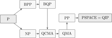
Every solid arrow means containment. Transitive containments are omitted, and spatial position has no set-theoretic meaning. The equality $\mathrm{QIP}=\mathrm{PSPACE}$ is known; strictness of the displayed containments is generally not.

In formulas, the main paths are

$$\begin{aligned} \mathrm P &\subseteq \mathrm{BPP} \subseteq \mathrm{BQP}, \\ \mathrm{BQP} &\subseteq \mathrm{QCMA} \subseteq \mathrm{QMA}, \\ \mathrm{QMA} &\subseteq \mathrm{PP} \subseteq \mathrm{PSPACE}. \end{aligned}$$

and

$$\mathrm P \subseteq \mathrm{NP} \subseteq \mathrm{QCMA}.$$

A tighter counting upper bound

$$\mathrm{BQP} \subseteq \mathrm{AWPP} \subseteq \mathrm{PP}$$

is known, but PP is more commonly used for a first map. The equality

$$\mathrm{QIP} = \mathrm{PSPACE}$$

is discussed below.

What remains open

No unconditional theorem currently establishes any of the following strict inequalities:

• $\mathrm{BPP}\neq\mathrm{BQP}$;
• $\mathrm{NP}\not\subseteq\mathrm{BQP}$;
• $\mathrm{BQP}\not\subseteq\mathrm{NP}$;
• $\mathrm{QCMA}\neq\mathrm{QMA}$;
• $\mathrm{BQP}\neq\mathrm{PSPACE}$.

It is also unknown whether P equals NP. Diagrams that draw separate regions for these classes often encode conjectures, not proved set relations.

The existence of compelling BQP algorithms is evidence of quantum advantage under current knowledge. It is not a proof that the same problems lack all classical polynomial-time algorithms.

Oracle Separations

An oracle $A$ is an idealized black box that answers a specified query at unit cost. The notation

$$\mathrm{BQP}^A$$

means BQP machines granted access to $A$; other classes receive the same oracle under their own query rules.

Oracle results can prove that one computational model exploits black-box structure more efficiently than another:

• Simon’s period-finding problem gives an oracle setting with polynomial quantum queries and exponentially many randomized classical queries.
• Raz and Tal constructed an oracle $A$ for which

$$\mathrm{BQP}^A \not\subseteq \mathrm{PH}^A,$$

where PH is the polynomial hierarchy.

• Aaronson and Kuperberg gave a quantum-oracle separation between QMA and QCMA.

These are rigorous separations in relativized or black-box models. They do not prove

$$\mathrm{BPP}\neq\mathrm{BQP}$$

or

$$\mathrm{QCMA}\neq\mathrm{QMA}$$

without an oracle. An oracle may also hide the physical cost of loading data or evaluating the queried function.

Query Complexity owns fixed black-box measures and the polynomial, adversary, and hybrid certificates used to prove matched-access query bounds. This page retains relativization and the distinction between oracle-world and unrelativized class claims.

Lower Bounds and Limitations owns the proof-technique and cross-resource implications of limitations on advantage claims; this page retains class definitions, containments, reductions, completeness statements, and the exact qualification of oracle-world evidence.

The right conclusion is methodological: any proof technique that behaves identically in every oracle world cannot settle a statement contradicted in one of those worlds. Oracle evidence can reveal mechanisms and barriers without resolving the ordinary class separation.

The Local Hamiltonian Problem

The $k$-local Hamiltonian problem is the canonical QMA-complete problem and the quantum analogue of classical constraint satisfaction.

An input describes

$$H = \sum_{j=1}^{m}H_j$$

on $n$ qubits, where $m=\operatorname{poly}(n)$ and each term $H_j$ acts nontrivially on at most $k$ qubits. The term entries and thresholds are specified with polynomially many bits.

Given numbers $a<b$ satisfying

$$b-a \geq \frac1{\operatorname{poly}(n)},$$

decide between

$$\begin{aligned} \text{YES:}\quad \lambda_{\min}(H) &\leq a, \\ \text{NO:}\quad \lambda_{\min}(H) &\geq b. \end{aligned}$$

Inputs with ground energy strictly between $a$ and $b$ violate the promise and may receive either answer.

Why it is in QMA

Merlin sends a purported low-energy state $\rho$. Arthur estimates its energy using polynomial resources, for example by sampling normalized local terms or by a suitable phase-estimation construction.

For a simple term-sampling verifier, shift and rescale so

$$0\leq H_j\leq I.$$

Choose $j$ uniformly and perform the two-outcome measurement

$$\{I-H_j,H_j\},$$

accepting on the first outcome. Then

$$\Pr[\text{accept}\mid\rho] = 1-\frac{\operatorname{Tr}(H\rho)}m.$$

A yes-instance has a witness with energy at most $a$. On a no-instance, the variational principle gives

$$\operatorname{Tr}(H\rho) \geq \lambda_{\min}(H) \geq b$$

for every witness. The acceptance gap is at least

$$\frac{b-a}{m},$$

which is inverse polynomial and can be amplified.

Why it is QMA-hard

The Feynman–Kitaev circuit-to-Hamiltonian construction encodes the history of a verifier computation. If

$$\lvert\psi_t\rangle = U_tU_{t-1}\cdots U_1 \lvert\psi_0\rangle,$$

the associated history state has the form

$$\lvert\eta\rangle = \frac1{\sqrt{T+1}} \sum_{t=0}^{T} \lvert t\rangle_{\mathrm{clock}} \lvert\psi_t\rangle_{\mathrm{work}}.$$

Local penalty terms enforce valid initialization, clock motion, gate propagation, and final acceptance. A verifier with an accepting witness produces a low-energy history state; soundness forces higher energy when no witness is accepted.

Kitaev’s construction established QMA-completeness for a constant-locality Hamiltonian. Kempe, Kitaev, and Regev proved that 2-local Hamiltonian on qubits is already QMA-complete.

Physical interpretation and limits

QMA-completeness is a worst-case statement about an inverse-polynomial-precision decision problem. It does not imply:

• every local Hamiltonian used in physics is hard;
• one-dimensional, commuting, stoquastic, gapped, or integrable subclasses all have the same complexity;
• preparing any ground state is equivalent to solving the decision problem;
• a variational method fails on every useful instance;
• finite-temperature observables inherit QMA-completeness automatically.

Locality is not enough by itself to guarantee tractability. Additional geometry, interaction type, symmetry, gap, sign structure, approximation scale, and input family can change the complexity.

Lattice Models Overview owns the physical language of local lattice Hamiltonians. This page owns the promise problem and its verifier complexity.

Adiabatic Quantum Computation owns the computation-model semantics and constructive circuit/history-state equivalence for a declared path. This page retains BQP and QMA definitions, Local Hamiltonian promise problems and completeness, and worst-case interpretation; deciding a low-energy promise problem is not the same task as following a supplied gapped path.

Quantum Interactive Proofs

In a quantum interactive proof, a computationally unbounded prover exchanges polynomial-size quantum messages with a polynomial-time quantum verifier. The verifier must satisfy completeness against an honest prover and soundness against every cheating strategy.

The class QIP contains problems with such polynomial-round protocols. Interaction appears much stronger than a single QMA witness, yet its exact power is known:

$$\mathrm{QIP} = \mathrm{PSPACE}.$$

The nontrivial direction is $\mathrm{QIP}\subseteq\mathrm{PSPACE}$, proved using semidefinite-program representations and matrix multiplicative weights. The reverse direction follows because classical interactive proofs satisfy $\mathrm{IP}=\mathrm{PSPACE}$ and are a special case of quantum interaction.

This equality does not say a standalone BQP machine solves PSPACE problems. The verifier receives help from an unbounded but untrusted prover and uses interaction to enforce soundness.

Related classes alter the protocol contract:

• QMA is the one-message quantum-witness model.
• QCMA keeps that message classical.
• QSZK additionally requires that interaction reveal essentially nothing beyond the truth of the claim.
• Multi-prover classes change the model by imposing separated provers and are not inferred from QIP alone.

The number and direction of messages, verifier randomness, entanglement assumptions, and zero-knowledge condition are all part of the class definition.

Reading a Quantum Speedup Claim

Complexity-class language is most useful when it prevents category errors. For any claimed quantum advantage, ask:

Question	Why it matters
What is the exact problem?	decision, search, function, and sampling tasks are not interchangeable
What is the input encoding?	amplitude or oracle access can hide data-loading cost
What is promised?	the algorithm may say nothing about off-promise inputs
Which resource is bounded?	query, gate, depth, and wall-clock complexity can differ
What is the comparator?	best known classical algorithm is not a lower bound
Is the result relativized?	oracle separation is not an ordinary class separation
Is the claim worst case or average case?	hardness and performance may live on different distributions
Is the circuit fault tolerant?	logical asymptotics omit physical overhead

The evidence taxonomy in Claims, Hype, and Evidence Standards distinguishes theorem, oracle result, resource estimate, experiment, and application claim.

Common Mistakes

• Treating BQP as the set of all problems a quantum computer might ever help with.
• Saying BQP is known to be strictly larger than BPP.
• Claiming Shor’s algorithm proves factoring is classically hard.
• Assuming NP-complete problems are efficiently solvable on quantum computers.
• Calling QMA “NP with a faster verifier” while omitting the quantum witness and soundness quantifier.
• Treating a classical description of a state as equivalent to a quantum witness.
• Forgetting the promise gap in local Hamiltonian.
• Inferring that every physical local Hamiltonian is QMA-hard.
• Reading a containment diagram as proof that every arrow is strict.
• Confusing PP’s tiny majority gap with bounded-error randomized computation.
• Treating an oracle query as a free physical subroutine.
• Concluding an unrelativized separation from an oracle separation.
• Interpreting $\mathrm{QIP}=\mathrm{PSPACE}$ as $\mathrm{BQP}=\mathrm{PSPACE}$.

Exercises

1. Amplify a BQP computation

A quantum circuit accepts yes-instances with probability at least $2/3$ and no-instances with probability at most $1/3$. Run it independently $k$ times and take a majority vote. Use Hoeffding’s inequality to bound the error.

Solution

For a yes-instance, let $X_i\in\{0,1\}$ be the acceptance indicator of run $i$. Then

$$\mathbb E[X_i] \geq \frac23.$$

The majority is wrong only if the sample mean falls by at least $1/6$. Hoeffding’s inequality gives

$$\overline X = \frac1k\sum_iX_i$$

and

$$\Pr\left[ \overline X\leq\frac12 \right] \leq e^{-k/18}.$$

The no-instance bound is identical after reversing acceptance and rejection. Thus $k=O(\log(1/\epsilon))$ repetitions reduce the error below $\epsilon$.

2. Prove three easy containments

Explain why

$$\mathrm{BPP} \subseteq \mathrm{BQP} \subseteq \mathrm{QCMA} \subseteq \mathrm{QMA}.$$

Solution

A quantum circuit can generate uniform random bits and reversibly simulate a classical randomized circuit, proving $\mathrm{BPP}\subseteq\mathrm{BQP}$.

A QCMA verifier may ignore its classical witness, so every BQP computation is a QCMA protocol with an empty witness.

For a QCMA protocol viewed as QMA, the verifier first measures the quantum witness register in the computational basis and then runs the QCMA verifier on the resulting string. A superposition therefore becomes a classical mixture of candidate strings. If no classical string succeeds above the soundness threshold, no superposition or mixture does either.

3. Keep the QMA quantifiers straight

For a no-instance, why is it insufficient to test the verifier on one plausible witness or on a finite list supplied by the algorithm designer?

Solution

QMA soundness requires

$$\forall\rho: \Pr[V_x(\rho)\text{ accepts}] \leq s.$$

The prover is adversarial and may send any state in the allowed witness space, not merely a witness anticipated by the verifier designer. Testing a selected list proves soundness only for that list.

Equivalently, acceptance is a positive linear functional of $\rho$, so the soundness question is the maximum acceptance probability over the entire state space. A valid proof must bound that maximum.

4. Verify local-Hamiltonian membership

Let

$$H=\sum_{j=1}^{m}H_j, \qquad 0\leq H_j\leq I.$$

The verifier chooses $j$ uniformly, measures $\{I-H_j,H_j\}$, and accepts on $I-H_j$. Derive the acceptance probability and the completeness–soundness gap.

Solution

Conditioned on $j$, the acceptance probability is

$$1-\operatorname{Tr}(H_j\rho).$$

Averaging uniformly,

$$\begin{aligned} \Pr[\text{accept}\mid\rho] &= \frac1m \sum_{j=1}^{m} \left[ 1-\operatorname{Tr}(H_j\rho) \right] \\ &= 1-\frac{\operatorname{Tr}(H\rho)}m. \end{aligned}$$

For a yes-instance, choose a witness with energy at most $a$, giving acceptance at least $1-a/m$. For a no-instance, every state has energy at least $b$, giving acceptance at most $1-b/m$. The gap is

$$\frac{b-a}{m}.$$

Because $m$ is polynomial and $b-a$ is inverse polynomial, the gap is inverse polynomial and can be amplified.

5. Identify the off-promise region

A local-Hamiltonian instance has thresholds $a=0.20$ and $b=0.25$. State what the algorithm must do when the ground energy is $0.18$, $0.23$, and $0.27$.

Solution

If $\lambda_{\min}=0.18\leq a$, the instance is a yes-instance and must be accepted with the promised completeness probability.

If $\lambda_{\min}=0.27\geq b$, it is a no-instance and must be rejected with the promised soundness probability.

If $\lambda_{\min}=0.23$, the input lies between $a$ and $b$ and violates the promise. The algorithm may accept or reject; its complexity guarantee imposes no condition there.

6. Interpret an oracle separation

Suppose there exists an oracle $A$ such that

$$\mathrm{BQP}^A \not\subseteq \mathrm{BPP}^A.$$

Which conclusion follows: an efficient quantum query algorithm outperforms every efficient randomized classical query algorithm relative to $A$, or $\mathrm{BQP}\neq\mathrm{BPP}$ without an oracle?

Solution

Only the first conclusion follows. The separation proves that the two relativized models differ when both receive unit-cost access to the same oracle $A$.

It does not prove an ordinary class separation. A nonrelativizing argument could behave differently when the oracle is replaced by an explicit function, and the explicit implementation cost may erase the query advantage.

7. Audit a containment diagram

A diagram asserts

$$\mathrm{NP} \subseteq \mathrm{BQP} \subsetneq \mathrm{QMA}.$$

Which parts are currently unjustified?

Solution

Neither displayed claim is known. It is open whether $\mathrm{NP}\subseteq\mathrm{BQP}$. Although $\mathrm{BQP}\subseteq\mathrm{QMA}$ is known, strictness is not; writing $\subsetneq$ overclaims a separation.

A safe statement is

$$\mathrm{BQP} \subseteq \mathrm{QMA},$$

together with an explicit note that the equality question is open. NP and BQP should not be ordered unless the diagram marks the relation as conjectural or unknown.

References

• S. Arora and B. Barak, Computational Complexity: A Modern Approach, Cambridge University Press, 2009, doi:10.1017/CBO9780511804090.
• E. Bernstein and U. Vazirani, “Quantum complexity theory,” SIAM Journal on Computing 26, 1411–1473, 1997, doi:10.1137/S0097539796300921.
• L. M. Adleman, J. DeMarrais, and M.-D. A. Huang, “Quantum computability,” SIAM Journal on Computing 26, 1524–1540, 1997, doi:10.1137/S0097539795293639.
• J. Watrous, “Quantum computational complexity,” in Encyclopedia of Complexity and Systems Science, 2009, arXiv:0804.3401.
• C. Marriott and J. Watrous, “Quantum Arthur–Merlin games,” Computational Complexity 14, 122–152, 2005, doi:10.1007/s00037-005-0194-x.
• S. Aaronson and G. Kuperberg, “Quantum versus classical proofs and advice,” Theory of Computing 3, 129–157, 2007, doi:10.4086/toc.2007.v003a007.
• J. Kempe, A. Kitaev, and O. Regev, “The complexity of the local Hamiltonian problem,” SIAM Journal on Computing 35, 1070–1097, 2006, doi:10.1137/S0097539704445226.
• R. Jain, Z. Ji, S. Upadhyay, and J. Watrous, “QIP = PSPACE,” Journal of the ACM 58, article 30, 2011, doi:10.1145/2049697.2049704.
• D. R. Simon, “On the power of quantum computation,” SIAM Journal on Computing 26, 1474–1483, 1997, doi:10.1137/S0097539796298637.
• R. Raz and A. Tal, “Oracle separation of BQP and PH,” Journal of the ACM 69, article 30, 2022, doi:10.1145/3530258.

See Also

• Algorithmic Primitives
• Shor Algorithm
• Circuit Model
• Universal Gate Sets
• Claims, Hype, and Evidence Standards
• Verification of Quantum Advantage
• Lattice Models Overview