Lower Bounds and Limitations

A lower bound limits a precisely declared task in a precisely declared resource. It does not automatically limit every implementation of a related task, nor does it automatically become a statement about gates, depth, energy, hardware time, or economic cost. Conversely, a quantum upper bound expressed in oracle calls or in the dimension of an amplitude-encoded input is not yet an end-to-end advantage. The missing steps may include obtaining the input, constructing the access interface, preparing states, compiling calls, extracting the requested output, controlling errors, repeating attempts, and verifying an accepted answer.

This page provides the implication discipline needed to carry a theorem across those boundaries. Its examples include no-fast-forwarding, generic state preparation, supplied quantum random-access memory, explicit-output and tomography costs, access-matched dequantization, noise-induced sampling overhead, relativized complexity evidence, and query-to-runtime conversion. The aim is neither to dismiss useful abstractions nor to replace them with one all-inclusive cost metric. It is to preserve what each result actually proves while making every additional conversion assumption visible.

The recurring rule is simple: freeze the computational contract, name the bounded resource, preserve the quantifiers, and demand a separate lemma for every change of resource. A theorem, a parameter-counting fact, a conditional conclusion, oracle evidence, and an empirical observation are different kinds of support. They can complement one another, but none may silently impersonate another.

Required background. Query Complexity supplies fixed-oracle resource measures and lower-bound proof vocabulary. Classical Information Review supplies the matched input, output, representation, accuracy, and total-cost contracts used throughout this page.

Cross-Resource Bounds on a Quantum Advantage Claim

The claim starts with a frozen contract

Let a computational claim concern a family labeled by a size parameter $n$ . Before quoting an asymptotic expression, specify the valid instances $x\in D_n$ , any promise $P_n(x)$ , the access map supplied to the algorithm, the required output relation $R_n(x)$ , the accuracy convention, and the accepted failure probability. A bound such as $Q(n,\epsilon)=\Omega(n)$ has meaning only inside that record. Changing from a bit oracle to coherent sample-and-query access, from an explicit vector to one expectation value, or from worst-case to average-case instances changes the problem rather than merely changing notation.

The comparison class must be frozen at the same time. A quantum circuit given a populated coherent data structure is not matched by a classical algorithm charged for reading an unindexed file. A quantum algorithm returning a state is not matched by a classical algorithm required to print every coordinate. A device experiment reporting the best observed sample is not matched by a classical solver required to certify optimality. The Claims, Hype, and Evidence Standards page owns the reporting language; here the concern is the formal implication beneath that language.

The contract also identifies the cost boundary. A theorem may count calls to $O_x$ while declaring every inter-query unitary free. A compiled analysis may count logical Clifford and non-Clifford gates but omit physical decoding latency. A benchmark may include queueing, calibration, retries, and verification. None of these boundaries is intrinsically wrong. Trouble begins when a conclusion is carried from one boundary to another without a proved reduction, an implementation model, or measured evidence.

A lower bound is not an end-to-end conclusion

Suppose every algorithm in a model requires at least $Q_*(n)$ oracle calls. This proves a lower bound on that named query resource. It may support a gate lower bound if every valid implementation necessarily expends a proved number of gates per distinguishable call and if cancellations or global implementations cannot evade the decomposition. Merely observing that one compiler uses $C(n)$ gates per call and multiplying $Q_*(n)C(n)$ does not prove that every implementation uses that product. The compiler supplies an upper bound on one implementation cost, not a universal per-call lower bound.

The reverse mistake is equally common. If an algorithm uses at most $Q(n)$ queries, an expensive known oracle circuit does not prove that the task itself is expensive: a different representation or an algorithm that never materializes that oracle may exist. Similarly, a worst-case hard family establishes existence of hard instances or distributions under its quantifiers. It does not make every instance hard, rule out structured exceptions, or determine typical performance on a chosen data distribution.

An end-to-end conclusion therefore needs a chain. Each link must state its direction: theorem to query count, interface implementation to logical resources, logical circuit to scheduled depth, scheduled computation to physical cycles, noisy execution to repetitions, and measured record to accepted answer. If one link is absent, the correct result is not “zero cost” but “conclusion unavailable at this boundary.”

The Eleven-Field Lower-Bound Claim Record

Recording a theorem before interpreting it

The record below is deliberately longer than a complexity label. Each row closes a loophole that otherwise permits an unlicensed change of problem, model, or conclusion. A field may be “not specified,” “excluded by the model,” or “not measured,” but those answers are not interchangeable with zero.

Claim field	Required content
Task, family, promise, and size variables	Name the relation or estimation task, the family $D_n$ , all promises, and every asymptotic variable rather than using one informal problem label.
Instance or input distribution	State worst case, average case under a named distribution, smoothed analysis, or one finite instance; retain adversarial choices and independence assumptions.
Representation, access, and supplied capabilities	Define classical storage, samples, coherent queries, inverse or controlled access, precision, preparation, and which construction costs are supplied.
Output and acceptance condition	Distinguish a state, one sample, an observable, a certificate, an implicit data structure, and an explicit classical description; give the verifier.
Error, success, and confidence	Give the norm or loss, additive or relative tolerance, per-attempt success, target confidence, and whether bias is permitted.
Bounded resource and unit of cost	Name queries, inspections, copies, measurements, gates, depth, qubits, cycles, time, energy, money, or cost per accepted answer and define one unit.
Upper or lower statement and asymptotic regime	State the inequality direction, parameter range, constants if material, limiting regime, and whether the statement is exact, asymptotic, or finite.
Quantifier order and hard-family scope	Preserve “for every algorithm there exists an instance,” distributional quantifiers, advice, uniformity, and whether one family or every instance is covered.
Reduction or implementation direction	Record which problem or resource maps to which, the overhead, success preservation, and whether the map is an upper-bound construction or lower-bound reduction.
Matched comparison class	Give the classical or quantum competitor the same input, output, accuracy, confidence, preprocessing, reuse, and accepted-answer boundary.
Licensed conclusion and excluded conclusions	Write the narrow claim supported by the preceding fields and explicitly list nearby gate, depth, runtime, physical, typical-case, or universal claims not established.

A robust claim can now be audited locally. If its lower-bound row says “oracle queries,” its conclusion may not say “seconds” unless later rows provide the conversion. If its output row says “quantum state,” it may not be compared with explicit vector writeout. If its quantifier row says “there exists a sparse Hamiltonian family,” the conclusion may not say “all Hamiltonians.” This disciplined record is not rhetorical caution; it is the mathematical type information required for valid implication.

Resources, Quantifiers, and Licensed Implications

Resource currencies are distinct

The following currencies answer different questions. “Dominant cost” is an empirical or model-dependent finding, not a reason to erase the other columns.

Resource currency	One counted unit	Needed contract	A valid implication	What does not follow	Typical owner
Input inspections and preprocessing	Read, sample, update, or arithmetic operation before governed execution	Storage format, precision, build algorithm, memory, reuse count	A proved preprocessing lower bound limits pipelines charged for that build	It does not apply when the data structure is genuinely supplied or reused under a different boundary	Classical Information Review
Oracle queries	One call to a fully defined access transformation	Registers, full-space action, precision, inverse/control licenses	A query lower bound limits algorithms in that fixed oracle model	It is not automatically a gate, depth, time, or hardware lower bound	Query Complexity
Copies and measurements	One independent state copy or declared collective measurement block	State family, measurement class, adaptivity, metric, confidence	A copy lower bound limits the specified estimation or reconstruction task	It need not limit one prescribed observable or an already-known property	State and Shadow Tomography
Logical gates	One gate from a named fault-free library	Synthesis tolerance, oracle circuits, arithmetic, cleanup, connectivity convention	A circuit lower bound constrains logical implementations in that library	It gives neither parallel depth nor physical cycles by itself	Gate synthesis and algorithm owners
Critical-path depth	One dependency layer under a scheduling model	Parallelism, connectivity, communication, measurement and feed-forward rules	A depth bound limits latency in that logical schedule	It is not elapsed time without gate and classical-latency data	Compilation owners
Logical qubits	One simultaneously live encoded information unit	Workspace policy, uncomputation, mid-circuit reuse, code interface	A width bound constrains logical memory under that program model	It is not a physical-qubit count without a code and target error	Algorithm and fault-tolerance owners
Physical qubits and cycles	One device qubit or error-correction cycle	Architecture, code, decoder, physical error, target logical failure	A resource estimate describes one fault-tolerant realization and scenario	It is not a theorem for every architecture or a measured runtime	Resource Estimation Tools
Wall-clock or accepted-answer cost	Seconds, energy, money, or another declared operational unit per accepted result	Scheduling, calibration, retries, decoding, verification, availability	A measured or modeled total can support an end-to-end comparison inside its envelope	It does not follow from asymptotic query notation alone	Algorithmic Benchmarking

An advantage can grow in one currency and disappear in another. Query count, gate count, depth, and physical time therefore remain a vector-valued ledger until a declared objective licenses a scalar comparison.

Quantifier order and asymptotic variables

The phrases “hard in the worst case” and “requires $L(n)$ ” hide quantifiers. A common theorem has the form

\forall A\in\mathcal A_n:\quad \left[ \forall x\in D_n, \Pr[A(x)\in R_n(x)]\ge 1-\delta \right] \Longrightarrow \left[ \exists x\in D_n, C_A(x)\ge L(n) \right].

This is not the same as the existence of one $x$ hard for all algorithms, an average-case lower bound over a chosen distribution, or a claim that every $x$ is hard. Randomized and quantum lower bounds may quantify over internal randomness, measurement outcomes, distributions, advice, or approximation error in different orders. Restoring those quantifiers often dissolves an apparent contradiction between a worst-case theorem and an easy structured instance.

Dimension $d$ , sparsity $s$ , rank $r$ , condition number $\kappa$ , scaled time $\tau$ , accuracy $\epsilon$ , confidence $1-\delta$ , depth $L$ , and database size $N$ are distinct asymptotic variables. A speedup in $d=2^n$ is meaningful in $n$ only if access and output avoid costs proportional to $d$ ; conditioning or explicit writeout can dominate a favorable dimension dependence.

Reductions and the direction of implication

If instances of $A$ reduce to $B$ and a solver for $B$ would solve $A$ , a lower bound for $A$ may transfer to $B$ after the reduction overhead is accounted for. A construction of a $B$ solver from an $A$ solver instead gives an upper-bound route. “Equivalent” requires both directions with promises, errors, and overheads.

If one query can be implemented with at most $C$ gates, then $Q$ queries plus nonquery work give a gate upper bound for that program. A gate lower bound instead needs an unavoidable-implementation argument. Multiplying a lower bound by an upper-bound conversion cost is invalid lower-bound arithmetic.

The Quantum Oracles page owns interface equivalences and capability licenses. The Query Complexity page owns query reductions and lower-bound certificates. This page records when those results may cross into a new resource statement and when the implication stops.

Canonical Ownership and Exclusions

The specialist owner table

Cross-resource reasoning is clearest when each theorem retains a single canonical home. The owner column below identifies where definitions, proofs, algorithm details, or empirical workflows belong; the present page owns only the transfer rule or limitation indicated in the final column.

Specialist owner	Retained subject	This page uses only
Query Complexity	Fixed-oracle measures; polynomial, adversary, hybrid, and information certificates; reductions and composition	The warning that a query result does not cross resource boundaries without a conversion lemma
Hamiltonian Simulation Algorithms	Sparse and block-encoded models, normalization, simulation algorithms, precision bounds, hard families, and structured exceptions	The exact scope of no-fast-forwarding and its non-implications for gates or physical time
Quantum Linear Algebra and Quantum Machine Learning	QLSP and learning tasks, access, conditioning, rank, outputs, verification, and theorem-specific bounds	General loading, output, matched-access, and dequantization caveats
State Tomography and Shadow Tomography	Reconstruction metrics, measurement models, estimators, copy bounds, and prescribed-observable protocols	The distinction between explicit reconstruction and restricted outputs
Quantum Complexity Classes	Class definitions, containments, completeness, reductions, interactive proofs, and exact oracle-world statements	The distinction among unconditional, conditional, and relativized evidence
Limits of Error Mitigation and quantum-error-correction owners	Protocols, no-go theorem details, codes, thresholds, and fault-tolerant constructions	The separation of mitigation sampling overhead from conditional fault-tolerant achievability
Resource Estimation Tools and Algorithmic Benchmarking	Compiled physical ledgers, scenarios, executed comparisons, and accepted-answer workflows	The data required before logical counts support runtime or cost claims
Negative Results and Limitations and Verification of Quantum Advantage	Dated empirical records, reversals, evidence chains, and update triggers	Durable implication rules that remain valid when particular experiments change

This division prevents a limitations page from becoming a second textbook on every lower-bound method. It also prevents a specialist page from carrying an end-to-end conclusion beyond its model. Cross-links are transfers of prerequisites and interpretation, not transfers of canonical ownership.

Deliberate exclusions

This page does not reproduce the polynomial or adversary methods, prove a sparse-Hamiltonian theorem from first principles, survey Hamiltonian-simulation algorithms, teach tomography estimators, catalogue quantum-learning models, derive every mitigation no-go result, or provide a fault-tolerant resource worksheet. It does not maintain a dated list of failed quantum-advantage experiments. Those would duplicate pages whose assumptions and update cycles are more specialized.

The exclusions also protect against a subtler error: collecting different limitations into one universal impossibility theorem. A state-preparation counting bound, a tomography copy lower bound, a dequantization result, and a noise-induced sampling theorem concern different tasks and models. They may all apply to one proposed pipeline only after that pipeline is shown to satisfy every hypothesis. Their costs cannot be added, maximized, or multiplied until overlap, dependence, and reuse have been specified.

The dated Research records remain planned, so evolving lower-bound frontiers do not belong in a stable theory article or an invented link to an unimplemented page. Durable principles appear here; dated open problems and changing records wait for their authorized owners.

No-Fast-Forwarding in Its Exact Model

The sparse black-box theorem

Set $\hbar=1$ . In the standard sparse-entry model, a $d$ -sparse Hamiltonian $H$ is accessed through black boxes that identify and evaluate the nonzero entries of a requested row. The natural dimensionless evolution scale is

\tau=d\lVert H\rVert_{\max}t,

where $\lVert H\rVert_{\max}=\max_{j,k}|H_{jk}|$ and $t$ is the simulated time. The access model, normalization, initial-state convention, output channel, and approximation metric are part of the theorem. Rescaling $H$ while leaving $t$ unchanged does not preserve the same instance; the product entering $\tau$ is what matters.

The original sparse-Hamiltonian obstruction is an existence statement with a different normalization. Write $\sigma=\lVert H\rVert t$ for its operator-norm time so that it is not confused with the sparse-entry scale $\tau$ above. Berry, Ahokas, Cleve, and Sanders construct, for every positive integer $N$ , a row-computable $2$ -sparse hard Hamiltonian with $\sigma=\pi N/2$ . Simulating the resulting state to trace-distance error at most $1/4$ needs at least $\sigma/(2\pi)=N/4$ Hamiltonian queries. This exact constant belongs to $\sigma=\lVert H\rVert t$ , not to $d\lVert H\rVert_{\max}t$ .

There is a second obstruction, logically separate from the linear-in- $\tau$ one. In the sparse-entry model, Berry, Childs, and Kothari give nearly optimal algorithms and lower bounds that include an $\Omega(\tau)$ dependence in the relevant regime and a high-precision obstruction of order

\Omega\!\left(\frac{\log(1/\epsilon)}{\log\log(1/\epsilon)}\right)

for the stated approximation task and oracle family. A page should not fuse these into “time times precision” unless a theorem actually gives that product. Nor should it replace the black-box query unit with logical gates. The Hamiltonian Simulation Algorithms page owns the precise hard families, access oracles, normalization, algorithms, and error conventions.

Structured fast-forwardable exceptions

No-fast-forwarding is not a ban on exploiting structure. Diagonal Hamiltonians with efficiently computable eigenvalues, commuting families, free-fermion models, or other succinctly diagonalizable systems can admit circuits whose cost grows much more slowly than a generic evolution time. The relevant question is whether the structure and the transformation exposing it are supplied or efficiently computable under the declared input model.

Atia and Aharonov formalize fast-forwarding and relate it to exponentially precise energy measurement. They also identify structured fast-forwardable classes, including commuting local Hamiltonians and quadratic fermionic Hamiltonians under their hypotheses. These exceptions do not contradict a hard-family oracle theorem: the domain has changed from all admissible sparse black boxes to a narrower class with exploitable algebraic information.

The correct structured claim names the family and the cost of recognizing or exposing the structure. If an efficient diagonalizing circuit $V$ and eigenvalue function $\lambda(z)$ are supplied, then implementing $V^\dagger e^{-i\lambda(z)t}V$ can be inexpensive even for large $t$ . If finding $V$ is itself the hard task, the same display is not an algorithm. A promise written only in prose, with no access mechanism for the promised information, cannot license a fast-forwarding conclusion.

What no-fast-forwarding does not imply

The theorem does not imply that every Hamiltonian requires $\Omega(t)$ gates, that physical systems cannot evolve for time $t$ without performing a digital simulation, or that an analog simulator must wait a time equal to a chosen dimensionless normalization. It does not turn oracle queries into circuit depth, energy, or dollars. It also does not rule out task-specific algorithms that estimate one property of $e^{-iHt}|\psi\rangle$ without producing a full simulation channel.

One should therefore report no-fast-forwarding in two sentences. The first states the theorem: a named hard family in a named sparse black-box model requires the stated number of oracle calls at the stated error. The second states the transfer limit: circuit, physical-time, and structured-family conclusions require additional implementation or reduction arguments. This qualification preserves a strong theorem instead of weakening it with an overbroad interpretation.

Input Access and State-Preparation Bottlenecks

Generic state descriptions and circuit synthesis

An arbitrary normalized pure state on $n$ qubits has $2^{n+1}-2$ real degrees of freedom after normalization and global phase are removed. A generic classical description therefore has exponential length in $n$ . In a declared exact circuit model consisting of arbitrary one-qubit gates and CNOTs, parameter counting and constructive synthesis show an exponential generic preparation cost. Shende, Bullock, and Markov give asymptotically optimal state-initialization circuits and matching exponential-order lower-bound reasoning for that model.

This is a counting fact about almost all states in a continuous family and an exact gate model. It is not a lower bound for every named state, for approximate preparation under every metric, or for states arriving from a physical source. The computational-basis state $|0^n\rangle$ , a stabilizer state, a matrix-product state of controlled bond dimension, or a state generated by a short known circuit occupies a highly structured subset. A generic-state statement that omits “generic,” “exact,” or the gate library changes its quantifiers.

Precision remains explicit: continuous rotations are ideal primitives here, whereas a discrete fault-tolerant library adds synthesis error and cost. Approximation can reduce preparation cost, so parameter counting alone does not choose a norm or physical method.

Structured loaders and succinct generators

Structure can replace an exponentially long table with a short program. If probabilities arise from an efficiently integrable distribution, Grover and Rudolph give a recursive state-preparation construction based on efficiently computed interval integrals. Other structured routes use arithmetic circuits, symmetries, tensor networks, generative models, or a short dynamical preparation. Each route is an algorithm only when its classical computations, precision, ancillas, and reversible cleanup are included.

A succinct generator changes the input representation. It does not refute a lower bound for unstructured amplitude lists, and the unstructured bound does not rule out the generator. The same distinction applies to an already-quantum input $|x\rangle$ produced upstream. If the scientific task genuinely begins with that state, preparation may be outside the boundary; if the claim concerns classical data stored on disk, silently treating $|x\rangle$ as free is a mismatch.

Physical preparation is a third contract. Cooling, heralding, adiabatic loading, or an upstream quantum process has fidelity, acceptance, and repetition costs outside a one-qubit-plus-CNOT count. The interface must state copy availability and error propagation.

QRAM as a supplied interface

Quantum random-access memory is often represented by a coherent map from an address register to stored data. The bucket-brigade proposal of Giovannetti, Lloyd, and Maccone uses $O(N)$ physical memory or switching elements for $N$ locations while arranging only $O(\log N)$ active routing elements along a query path. That architectural statement is neither an $O(\log N)$ construction of an arbitrary database nor a proof that fault-tolerant queries are cheap.

When a theorem assumes QRAM, say “given a populated coherent random-access interface with the stated precision and action.” Construction, population, refresh, control, and fault tolerance move to a separate ledger; an end-to-end claim must say whether they are included or amortized.

The classical comparator must receive matched access. It may be appropriate to give both algorithms the same preprocessed tree or random-access table and charge only online calls. It may instead be appropriate to charge both for building their structures from raw records. Comparing supplied quantum access with unstructured classical access changes two variables at once and cannot isolate a quantum advantage.

Construction, reuse, and amortization

Let $B_Q$ and $B_C$ be quantum and classical build costs, let $R$ be the number of reused problem instances or queries served by one build, and let $U_Q$ and $U_C$ be the corresponding online costs per use. A simple amortized boundary is

\bar C_Q(R)=\frac{B_Q}{R}+U_Q, \qquad \bar C_C(R)=\frac{B_C}{R}+U_C.

The break-even reuse count depends on all four quantities and exists only when their differences have the right signs. If the data change between calls, $B_Q$ may recur. If updates are local, a dynamic maintenance cost may replace a full rebuild. If preparation consumes the stored state, the supposed reuse may be physically unavailable. “One-time preprocessing” is therefore a claim about workload and persistence, not a mathematical constant that can always be discarded.

Arbitrary classical records can create an inspection floor, but this intuition is not a universal $\Omega(N)$ theorem: sampling, promises, succinct encodings, and property testing can change the task. Name the input distribution and accepted output before invoking a loading barrier.

Output, Readout, and Tomography Bottlenecks

A quantum state is not a classical vector

The output of the quantum linear-systems algorithm of Harrow, Hassidim, and Lloyd is a quantum state proportional to the solution vector under strong access, sparsity, conditioning, and precision assumptions. That state can support expectation estimation or another coherent subroutine. It is not a printed list of all solution coordinates. Requiring an explicit $d$ -coordinate vector defines a larger output task with at least the time needed to write its chosen finite-precision representation.

Six output contracts must stay separate: a prepared state, one sample from a measurement, one expectation value, a prescribed family of observables, a certificate accepted by a verifier, and a complete classical vector or density matrix. They have different information content and can have different optimal methods. An algorithm that produces one of them has not failed because it does not produce another; the comparison must ask for the output the application actually consumes.

Trace distance, total variation, expectation error, coordinatewise vector error, and objective suboptimality are not interchangeable. Any norm conversion and its dimension factor belong in the implication chain.

The full-tomography output contract

Full state tomography asks for a classical description of an unknown $d$ -dimensional density operator from copies under a specified measurement model and loss. For rank- $r$ states, the number of real parameters is of order $rd$ , but parameter count alone does not settle the statistical rate. Haah, Harrow, Ji, Wu, and Yu establish sample-optimal bounds: for full-rank states and trace-distance error $\epsilon$ , collective measurements require $\Omega(d^2/\epsilon^2)$ copies, while an upper bound of order $d^2\log(d/\epsilon)/\epsilon^2$ is achievable; rank-sensitive bounds scale with $rd/\epsilon^2$ up to the stated logarithmic factors and regimes.

Measurement restrictions matter. O’Donnell and Wright develop efficient tomography procedures and rank-sensitive guarantees, whereas Lowe and Nayak prove stronger lower bounds for nonadaptive single-copy measurements: under their trace-distance formulation, arbitrary single-copy measurements require $\Omega(r^2d/\epsilon^2)$ samples, and constant-outcome measurements require $\Omega(r^2d^2/\epsilon^2)$ in the stated regimes. These results cannot be mixed without retaining rank, metric, adaptivity, and collective-versus-single-copy access.

A tomography bound applies to full classical reconstruction in its metric, not unchanged to two-hypothesis discrimination, one observable, a promised stabilizer description, or a supplied preparation circuit. State Tomography owns those models.

Targeted observables, samples, and shadows

Restricted outputs can be much cheaper than reconstruction. Given an unknown $D$ -dimensional state and $M$ known two-outcome measurements, Aaronson formulated shadow tomography: estimate all $M$ acceptance probabilities to additive error $\epsilon$ using a number of copies polylogarithmic in $D$ and $M$ in the original theorem, with a dependence of approximately $\widetilde O(\epsilon^{-4}\log^4 M\log D)$ . The output is the prescribed list of expectation estimates, not a full density matrix.

A classical-shadow protocol can cheaply estimate a governed observable family under favorable norms and measurements, but it does not grant arbitrary future queries. Shadow Tomography owns the protocol bounds.

Samples can also be the natural answer. If a downstream task consumes bit strings from a distribution, demanding a probability table of exponential length invents an unnecessary output requirement. Conversely, a few samples do not constitute a classical description, and reporting only the best sample can introduce selection bias unless the acceptance and stopping rules were frozen.

Random access and explicit writeout

An explicit output of $d$ coordinates with $b$ bits per coordinate contains $db$ output bits, so a sequential interface that physically writes one bit per step has an elementary $\Omega(db)$ writeout cost. This is an interface counting fact, not a theorem about the internal quantum computation. Parallel output changes depth but not total output size; compressed output changes the task and needs a decoder and fidelity guarantee.

Random access does not allow an exponential classical message to be hidden in a small quantum state while preserving reliable recovery of every bit. Nayak proves that an encoding of $N$ classical bits into $m$ qubits from which each bit can be recovered with success probability at least $p>1/2$ obeys

m\ge \bigl[1-H_2(p)\bigr]N,

where $H_2$ is binary entropy, under the random-access-code model. The theorem does not forbid quantum states from representing structured vectors compactly or supporting selected global observables. It limits a specific promise of reliable per-bit recovery.

Thus “the answer is stored in amplitudes” is incomplete. One must say which measurement or coherent consumer retrieves what information, with what copy count and success. If the intended use ultimately prints all coordinates, output size re-enters. If the intended use is a small prescribed observable family, tomography and writeout bounds may be irrelevant.

Dequantization under Matched Access

Sample-and-query access

Dequantization results often compare a quantum algorithm using amplitude access with a classical algorithm given a data structure supporting length-square sampling, entry queries, and norm information. For a vector $x\in\mathbb C^N$ , a typical classical interface can query $x_i$ , sample $i$ with probability $|x_i|^2/\lVert x\rVert_2^2$ , and return or estimate $\lVert x\rVert_2$ . Matrix versions add row-norm sampling and entry access. Precision, failure probability, build cost, storage, and update rules are part of this capability.

Tang used such access to give a quantum-inspired classical recommendation-system algorithm with polylogarithmic dependence on large dimensions under low-rank and approximation assumptions, narrowing the earlier exponential-separation narrative for that access model and output task. Chia, Gilyén, Li, Lin, Tang, and Wang developed a broader sampling-based sublinear low-rank matrix-arithmetic framework. Neither result begins with an ordinary flat file while the compared quantum algorithm begins with a free amplitude state.

Matched access does not require identical internal operations. It requires comparable supplied information and comparable charging. If the quantum interface can coherently prepare row states and their inverses, the classical side should receive the corresponding sampling/query data structure when the dequantization theorem assumes it. If building either structure is material to the application, both build ledgers should be included.

Rank, conditioning, precision, and preprocessing

Low rank is not one Boolean promise. Algorithms may depend on exact rank, stable rank, spectral decay, Frobenius norm, incoherence, or the quality of a truncated approximation. The condition number $\kappa$ controls amplification of small singular directions, while precision $\epsilon$ can enter polynomially. Hiding these factors behind “polylogarithmic in dimension” can reverse the practical or asymptotic comparison.

The Quantum Linear Algebra page owns QLSP-specific access, conditioning, state output, observables, and verification. The Quantum Machine Learning page owns task-specific kernels, losses, generalization, and dequantization. In particular, Huang, Broughton, Mohseni, Babbush, Boixo, Neven, and McClean show that the origin and amount of data can qualitatively change quantum-learning power; a classical-data dequantization result should not be universalized to arbitrary quantum data.

Preprocessing must be attached to the workload. A balanced binary tree may support polylogarithmic sampling and update operations but require linear work to populate from $N$ arbitrary entries. Over many online calls that build may amortize; over a single query it may dominate. A theorem conditioned on the data structure remains correct either way. Only the end-to-end claim changes.

The licensed conclusion of a dequantization

A sound conclusion has the form: under this sample-and-query interface, these rank, norm, conditioning, and precision promises, this output, and this accounting of preprocessing and reuse, a classical algorithm matches or narrows the stated quantum complexity advantage. That statement can be decisive. It identifies which claimed speedup came from unequal access or an implicit output rather than from quantum processing.

It does not prove that arbitrary quantum data are classically accessible, that every quantum machine-learning task is easy, that no polynomial improvement remains, or that a hardware experiment has no value. It may leave dependence on $\kappa$ , $1/\epsilon$ , rank, or large constants that matter in a different asymptotic regime. It may also compare query models without constructing an equally fast conventional memory system.

Dequantization is therefore a matched-model result, not a universal adjective applied to an application area. The scientific response is to update the claim record: narrow the task, expose the access assumption, change the baseline, and identify any surviving separation. Treating the result as either irrelevant or globally fatal discards the information it actually supplies.

Noise, Mitigation, and Fault-Tolerant Overhead

Noise contracts and distinguishability

A noise limitation begins with a channel family. For ideal hypothesis states $\rho_0,\rho_1$ and depth- $L$ process $\mathcal N_L$ , suppose the declared model proves

\bigl\lVert\mathcal N_L(\rho_0)-\mathcal N_L(\rho_1)\bigr\rVert_1 \le \eta_L\lVert\rho_0-\rho_1\rVert_1, \qquad 0\le\eta_L\le 1,

Then distinguishability may shrink with $\eta_L$ . The conclusion still depends on channel, circuit, controls, measurement, estimator, and ancillary resources; a depolarizing theorem is not a coherent-error theorem.

For an unbiased bounded estimator with single-shot variance $\sigma^2$ , independent repetitions $M$ give standard error $\sigma/\sqrt M$ . If noise attenuates the mean by $\eta_L$ and mitigation rescales by $1/\eta_L$ , the variance is amplified by $1/\eta_L^2$ in this elementary model. Holding a target standard error $\epsilon$ can then require

M\ge \frac{\sigma^2}{\eta_L^2\epsilon^2}.

This calculation is a transparent propagation of declared assumptions. It is not a universal lower bound for biased estimators, collective strategies, error-detecting circuits, or different observables.

Mitigation, postselection, and sampling overhead

Error mitigation seeks a less biased estimate without encoding a fully corrected logical computation. Zero-Noise Extrapolation owns finite-instance physical scaling, effective-gain and coordinate-zero inference, covariance, validation, and abstention decisions; this page retains formal asymptotic lower-bound assumptions, resource regimes, and limitation scope. Temme, Bravyi, and Gambetta introduced zero-noise extrapolation and probabilistic error cancellation for short-depth circuits. In probabilistic cancellation, quasiprobability weights can enlarge variance; in extrapolation, coefficient growth and model mismatch can do the same. Postselection raises conditional fidelity only by discarding runs, so its acceptance probability belongs in cost per accepted estimate.

Formal limits are correspondingly scoped. Takagi, Endo, Minagawa, and Gu derive fundamental sampling-cost bounds for broad mitigation protocols, including exponential overhead for layered circuits under local depolarizing noise in the stated setting. Tsubouchi, Sagawa, and Yoshioka use quantum estimation theory to obtain a universal cost bound for unbiased observable estimation under their generic layered Markovian model. Quek, Stilck França, Khatri, Meyer, and Eisert establish tighter worst-case limitations, including shallow circuit families requiring superpolynomial samples for broad mitigation classes under their hypotheses.

These are strong no-go results for specified protocols, noise, circuits, and estimators, not every observable on every noisy circuit. Retain the worst-case or family quantifier; structure, symmetry, or error detection may change the cost.

Mitigation, fault tolerance, and surviving routes

Mitigation and fault-tolerant correction change different contracts. Mitigation transforms data from noisy executions and pays bias, variance, calibration, or acceptance overhead. Fault tolerance encodes logical information, repeatedly extracts syndromes, decodes, and implements logical operations so that the total failure can be suppressed below a target—conditional on local noise, threshold, decoder, architecture, and resource assumptions.

A mitigation lower bound therefore does not contradict a threshold theorem. It says a class of unencoded estimation strategies pays a cost under a named noisy process. A threshold theorem supplies a surviving route by changing the implementation to an encoded one, usually with substantial qubit, gate, cycle, distillation, routing, and decoding overhead. Whether that route is advantageous is a resource-estimation question, not a logical contradiction.

Retain both ledgers: mitigation cost for a specified estimator and fault-tolerant cost for a logical program. Compare them only after matching accuracy, confidence, output, and hardware assumptions.

Complexity-Theoretic Barriers and Relativization

Class containments and unresolved separations

A complexity-class statement concerns languages or promise problems decidable by uniform machine families under a resource definition. Bernstein and Vazirani established the quantum complexity framework underlying BQP, while Adleman, DeMarrais, and Huang clarified machine amplitudes and containments such as algebraic-amplitude BQP within PP. These results define and bound computational power; they do not by themselves identify a practical speedup for a particular encoded dataset.

Containment, separation, completeness, and conditional hardness differ. For example, $\mathrm{BQP}\subseteq\mathrm{PP}$ is not an efficient classical simulation; completeness requires a named reduction, and conditional hardness retains its assumption.

In particular, no unconditional theorem currently proves

\mathrm{BPP}\ne\mathrm{BQP}, \qquad \mathrm{NP}\not\subseteq\mathrm{BQP}, \qquad\text{or}\qquad \mathrm{BQP}\not\subseteq\mathrm{PH}.

The Quantum Complexity Classes page owns the exact definitions and known containments. The limitation here is epistemic and formal: best-known algorithms, failed searches for simulations, and oracle separations are evidence, not proofs of these ordinary-world statements.

Oracle evidence

An oracle separation constructs a black box relative to which two relativized classes differ. Bennett, Bernstein, Brassard, and Vazirani showed, for a uniformly random oracle $A$ , that $\mathrm{NP}^{A}\not\subseteq\mathrm{BQP}^{A}$ with probability one. This demonstrates limits of black-box quantum search and supplies evidence about possible class relationships. The oracle is part of the theorem; deleting its superscript changes the statement.

Raz and Tal proved that there exists an oracle $O$ for which

\mathrm{BQP}^{O}\not\subseteq\mathrm{PH}^{O}.

This resolves the relativized question they posed and constrains proof strategies that would hold uniformly relative to every oracle. It does not prove $\mathrm{BQP}\not\subseteq\mathrm{PH}$ without an oracle. Nor does it supply an executable implementation of $O$ whose gate cost preserves the oracle separation.

Oracle evidence identifies a clean model, proves a separation there, and excludes some general simulation arguments. Label it “oracle separation,” neither vague caveat nor unrelativized theorem.

Relativization limits proof techniques

Baker, Gill, and Solovay constructed oracles relative to which $\mathrm P=\mathrm{NP}$ and other oracles relative to which $\mathrm P\ne\mathrm{NP}$ . Consequently, a proof technique that relativizes in the relevant sense cannot settle the ordinary P-versus-NP question: the same reasoning would have to survive both oracle worlds. This is a barrier on a family of proof techniques, not evidence that the ordinary equality takes either value.

The same discipline applies in quantum complexity. If an oracle world separates BQP from PH, any proposed theorem placing BQP inside PH by a fully relativizing argument cannot be correct in full generality. A nonrelativizing technique might still establish an ordinary-world containment or separation. Algebraization, natural-proofs phenomena, and other barriers have their own hypotheses and should not be imported merely because the word “barrier” appears.

Complexity evidence can exclude reductions or simulations without assigning wall-clock cost. Implementation claims additionally need an explicit reduction and uniform encoding.

From Queries to Gates, Depth, and Runtime

Oracle implementations and call graphs

Suppose a logical algorithm makes $Q_j$ calls to each licensed oracle family $j$ , and a chosen compiler implements a call with $C_j$ logical gates. A complete upper-bound accounting identity for that compiled program is

G_{\mathrm{logical}} =G_{\mathrm{nonquery}} +\sum_j Q_jC_j +G_{\mathrm{control}} +G_{\mathrm{arithmetic}} +G_{\mathrm{cleanup}}.

The terms must not overlap: if oracle circuits already include their controls or cleanup, those costs are not added twice. Forward, inverse, controlled, powered, precision-dependent, and coherent-family calls may have different $C_j$ . Workspace that persists across calls changes both gates and live qubits.

This identity is an upper-bound ledger once every component is implemented. It does not turn a query lower bound into $\Omega(\sum_jQ_jC_j)$ , because $C_j$ is generally an upper bound for one decomposition. A universal gate lower bound needs a separate unavoidable-implementation argument. Similarly, treating $C_j=1$ is legitimate inside an oracle model but must be labeled as an abstract call, not a hardware gate.

A call graph reveals reuse and concurrency. Two nominal calls may share one prepared data structure; one logical call may invoke many physical memory operations; several commuting calls may run in parallel. Writing the graph before multiplying prevents both missing costs and invented products.

Gate count, depth, and scheduling

Gate count sums operations; depth finds a critical path through dependencies under a declared scheduling and connectivity model. If $Q$ calls occur in $R_Q$ serial query rounds, each implemented layer has depth at most $D_O$ , and nonquery work has scheduled depth $D_N$ , then one particular schedule has

D_{\mathrm{logical}}\le R_QD_O+D_N+D_{\mathrm{routing}}+D_{\mathrm{feedforward}}.

Using $Q D_O$ instead assumes all calls are serial. Using only $R_Q$ assumes the oracle layer itself has unit depth. Neither assumption should be hidden. Measurements can terminate a dependency chain, create a classical feed-forward delay, or permit qubit reuse; connectivity can turn a low-depth all-to-all circuit into a deeper routed circuit.

Depth still is not time. Logical gate types have different durations, error-correction gadgets may span different cycle counts, and concurrent operations compete for factories, buses, or control hardware. A depth bound can license a latency statement only after these timing and capacity constraints are supplied.

Logical-to-physical cost and accepted answers

A physical estimate chooses an architecture, code family, code distance, decoder, physical error model, target total failure, magic-state strategy, routing layout, cycle time, and classical-control latency. It then maps logical gates, depth, and live qubits into physical qubits and cycles. The Resource Estimation Tools page owns that scenario calculation; one estimate does not become a hardware-independent theorem.

Success and verification close the ledger. If independent attempts succeed with probability $p$ , the least $k$ giving confidence at least $1-\delta$ satisfies

1-(1-p)^k\ge 1-\delta.

Cost per accepted answer includes those attempts, state preparation, calibration, decoding, readout, classical verification, and rejected runs. Correlated failures or adaptive stopping require a different probability model. The Algorithmic Benchmarking page owns executed comparisons and uncertainty.

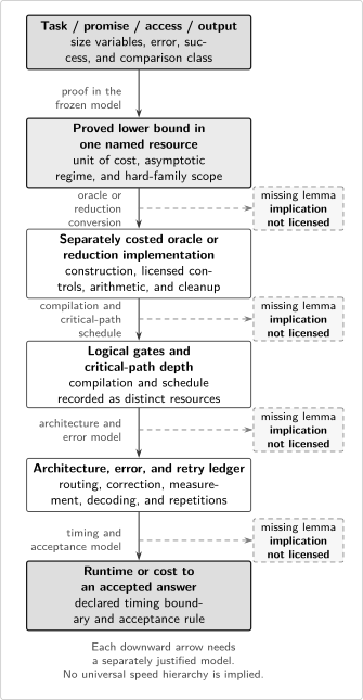
A vertical ledger showing the separately justified transitions from a computational contract to accepted-answer cost — A lower bound lives first in one named resource. Each arrow—from the frozen task and access contract to an oracle or reduction implementation, logical gates and critical-path depth, architecture and retry costs, and finally runtime or cost per accepted answer—needs a separately justified model or lemma. If that justification is absent, the cross-resource implication is not licensed.

Three Reproducible Finite Audits

Audit 1 — A no-fast-forwarding normalization ledger

Freeze $d=2$ , $\lVert H\rVert_{\max}=h=3/4$ , $t=16$ , and $\hbar=1$ . Direct substitution gives $\tau=dht/\hbar=24$ . A hypothetical observed or budgeted query count $Q=6$ therefore has the dimensionless ratio $Q/\tau=1/4$ . The audit checks normalization, units, and arithmetic only. One finite ratio neither proves the asymptotic no-fast-forwarding theorem nor shows that this particular Hamiltonian belongs to its hard family.

Audit 2 — An input-payload ledger

Freeze an explicit payload of $N=1024$ complex entries, with two signed or unsigned $16$ -bit components per entry under a declared fixed-point convention. The raw payload is $1024\times2\times16=32{,}768$ bits, or $4{,}096$ bytes, which is $4$ KiB. A binary address uses $\log_2N=10$ bits. A supplied-loader convention may exclude reading, building, and populating these payload bits from the online count; it does not erase storage, precision, maintenance, or fault-tolerant query costs from an end-to-end ledger.

Audit 3 — A query-to-logical-resource ledger

Freeze $Q=40$ calls arranged in ten serial query rounds. Let each query contribute $800$ gates, each query layer contribute depth $120$ , and let nonquery work contribute $12{,}000$ gates and depth $900$ . One attempt then has $44{,}000$ gates and depth $2{,}100$ . With independent per-attempt success $3/4$ , four attempts are necessary and sufficient to exceed $99\%$ confidence, giving conservative sequential totals of $176{,}000$ gates and depth $8{,}400$ . Runtime remains unavailable because no gate timings, architecture, routing, error-correction cycles, or classical latency were supplied.

The following dependency-free program recomputes all three ledgers from primitive inputs, checks units and identities with hard assertions, and prints only the governed sentinel.

const assert = (condition, label) => {
  if (!condition) throw new Error(label);
};

const normalization = {
  d: 2,
  h: 3 / 4,
  t: 16,
  hbar: 1,
  queries: 6,
  units: { d: 'dimensionless', h: 'inverse-time', t: 'time', hbar: 'dimensionless' },
};
const tau = normalization.d * normalization.h * normalization.t / normalization.hbar;
assert(normalization.units.h === 'inverse-time' && normalization.units.t === 'time', 'normalization units');
assert(tau === 24, 'scaled time');
assert(normalization.queries / tau === 1 / 4, 'query ratio');

const payload = { entries: 1024, componentsPerEntry: 2, bitsPerComponent: 16 };
const payloadBits = payload.entries * payload.componentsPerEntry * payload.bitsPerComponent;
const payloadBytes = payloadBits / 8;
const payloadKiB = payloadBytes / 1024;
const addressBits = Math.log2(payload.entries);
assert(Number.isInteger(addressBits), 'address width');
assert(payloadBits === 32768, 'payload bits');
assert(payloadBytes === 4096 && payloadKiB === 4 && addressBits === 10, 'payload units');

const conversion = {
  queries: 40,
  serialQueryRounds: 10,
  gatesPerQuery: 800,
  depthPerQueryLayer: 120,
  nonqueryGates: 12000,
  nonqueryDepth: 900,
  successPerAttempt: 3 / 4,
  targetConfidence: 0.99,
};
const gatesPerAttempt = conversion.queries * conversion.gatesPerQuery + conversion.nonqueryGates;
const depthPerAttempt = conversion.serialQueryRounds * conversion.depthPerQueryLayer + conversion.nonqueryDepth;
const attempts = Math.ceil(Math.log(1 - conversion.targetConfidence) / Math.log(1 - conversion.successPerAttempt));
assert(gatesPerAttempt === 44000 && depthPerAttempt === 2100, 'per-attempt resources');
assert(attempts === 4, 'attempt count');
assert(1 - (1 - conversion.successPerAttempt) ** attempts >= conversion.targetConfidence, 'confidence attained');
assert(1 - (1 - conversion.successPerAttempt) ** (attempts - 1) < conversion.targetConfidence, 'attempt count minimal');
assert(gatesPerAttempt * attempts === 176000, 'sequential gates');
assert(depthPerAttempt * attempts === 8400, 'sequential depth');
const runtime = null;
assert(runtime === null, 'runtime requires timing and architecture inputs');

console.log('Lower-bound finite audits: PASS');

The executable audit is a consistency check, not evidence for asymptotic hardness, hardware performance, or quantum advantage. Its purpose is to catch unit errors, missing terms, incorrect retry arithmetic, and an invented runtime before those mistakes enter a larger claim.

Common Cross-Resource Claim Failures

The comparison table summarizes seven recurring barriers. Each row states the evidence type and the largest nearby conclusion it can support without an additional bridge.

Barrier	Frozen contract	Evidence kind	Licensed conclusion	Unlicensed leap
No-fast-forwarding	Sparse black-box Hamiltonian, scaled time, state/channel error, hard family	Oracle-query lower-bound theorem	Generic simulators in that model cannot beat the stated time or precision dependence over the hard family	Every structured Hamiltonian needs linear gate depth or physical time
Generic preparation	Arbitrary exact $n$ -qubit pure state, one-qubit gates plus CNOTs	Parameter counting and circuit synthesis	Almost all exact states need exponentially many parameters and entangling gates in that model	Every scientifically relevant or approximately prepared state is hard
Supplied coherent memory	Fully defined populated QRAM action, precision, reuse	Interface assumption plus architecture estimate	Online query analysis is conditional on that supplied interface	Arbitrary data are loaded, maintained, and fault protected in logarithmic total cost
Explicit output or tomography	State family, requested classical description, metric, measurement class	Output-size fact or copy lower-bound theorem	Reconstruction requires the stated output bits or copies	One observable, one sample, or a prescribed shadow task has the same cost
Dequantization	Matched sample-and-query access, rank, conditioning, precision, output	Classical upper-bound construction	The corresponding quantum advantage narrows under the matched model	Arbitrary quantum data or all quantum learning are classically easy
Noise and mitigation	Channel, circuit family, estimator, bias, target error, allowed protocol	Variance calculation or scoped no-go theorem	The named strategy pays the proved sampling or acceptance overhead	All mitigation fails, or fault-tolerant correction is contradicted
Complexity and implementation	Language or promise problem, oracle/reduction, then compiled architecture	Containment, conditional or oracle evidence, plus separate estimates	The exact class or oracle statement and any explicitly modeled conversion	An unconditional class separation, universal circuit lower bound, or wall-clock verdict

Upper bound presented as impossibility. The best known cost is not a lower bound. “No faster method is known” is empirical; impossibility needs a proof with the relevant quantifiers.

Worst case presented as every case. “For every algorithm there exists a hard input” permits easy structured cases. Typical performance needs a distributional result.

A product of unlike inequalities. From $Q\ge Q_*$ and an implementation using at most $C$ gates per query, $G\ge Q_*C$ does not follow. Prove unavoidable gate cost or leave it open.

Free input on only one side. Match or separately charge amplitude access, QRAM, samples, preprocessing, and norm information; keep supplied-access conclusions conditional.

Output substitution. A state, expectation, sample, certificate, and full description differ. Tomography does not bound one observable, and an explicit-output baseline does not match a state output.

Noise theorem without its model. Retain locality, Markovianity, circuit family, estimator bias, and allowed controls; distinguish worst-case theorem from finite observation.

Oracle world presented as the ordinary world. Superscripts such as $O$ are mathematical content. Oracle separations constrain relativizing arguments but do not settle ordinary-world relations.

Logical depth presented as seconds. Runtime additionally needs scheduling, durations, communication, correction, decoding, repetitions, and verification. Otherwise it is unavailable.

Exercises

1. Restore the quantifiers in a lower-bound claim

A draft says, “Simulating a sparse Hamiltonian for scaled time $\tau$ always needs at least $\tau/(2\pi)$ quantum gates.” Diagnose its conflated normalization and rewrite it using $\sigma=\lVert H\rVert t$ as licensed by the original sparse no-fast-forwarding result. Then list three unavailable conclusions.

Solution

For every positive integer $N$ , there exists a row-computable $2$ -sparse Hamiltonian in the stated black-box model, with an associated initial-state task at operator-norm time $\sigma=\lVert H\rVert t=\pi N/2$ , such that any algorithm producing a state within trace distance $1/4$ of the target needs at least $\sigma/(2\pi)=N/4$ Hamiltonian queries. The quantifiers are “for every $N$ , there exists a hard Hamiltonian, and every successful algorithm for it needs the stated queries,” not “for every Hamiltonian.” The draft also changed queries into gates and replaced $\sigma$ by the distinct sparse-entry scale $\tau=d\lVert H\rVert_{\max}t$ .

Unavailable are an $\Omega(\tau)$ gate bound for every implementation, an $\Omega(t)$ physical-runtime bound, and hardness for every structured Hamiltonian. Each needs a separate implementation, timing, or structured-family theorem. Hamiltonian Simulation Algorithms owns the sparse theorem.

2. Audit a generic state-preparation statement

In the exact circuit model with arbitrary one-qubit gates and CNOTs, derive the parameter-count order for preparing a generic $n$ -qubit pure state from $|0^n\rangle$ . State why the conclusion does not apply to a state generated by a known polynomial-size circuit.

Solution

A vector in $\mathbb C^{2^n}$ has $2^{n+1}$ real coordinates. Normalization removes one degree of freedom and global phase removes another, leaving $2^{n+1}-2$ . An initial product state carries at most $2n$ relevant real parameters. In the standard exact one-qubit-plus-CNOT parameter-count argument, each additional CNOT can expose at most four new state parameters after redundant local freedoms are removed. If $k$ CNOTs prepare a generic state, then

2n+4k\ge 2^{n+1}-2, \qquad k\ge \frac{2^n-n-1}{2}=\Omega(2^n).

This exact-model statement permits much shorter structured or approximate preparations. A polynomial-size generator reaches only a structured subset and therefore does not contradict the generic bound. Shende, Bullock, and Markov own the synthesis result; this page owns its qualification.

3. Separate a quantum state from an explicit output

An algorithm prepares $|x\rangle=\sum_{i=0}^{d-1}x_i|i\rangle$ and estimates $\langle x|M|x\rangle$ to additive error $\epsilon$ . A comparison table says that it “returns the $d$ -component solution vector.” Diagnose the claim and give two legitimate output contracts.

Solution

Preparing $|x\rangle$ does not return an explicit list $(x_0,\ldots,x_{d-1})$ . Measurement exposes statistics of chosen observables, and amplitudes are not simultaneously readable coordinates. The table has substituted a larger classical-output task for the actual state-and-observable task.

One contract prepares a state within a named distance and estimates $\langle M\rangle$ to error $\epsilon$ and failure $\delta$ . Another outputs all $d$ complex coordinates to $b$ bits in a named norm, incurring explicit writeout of order $db$ . Quantum Linear Algebra owns state-output theorems; State Tomography owns reconstruction bounds.

4. Match access in a dequantization comparison

A quantum recommendation algorithm is given coherent row-state preparation in unit cost. Its classical comparator receives a flat array and is charged for building a length-square sampler. Specify a matched comparison, including preprocessing and reuse, and state the conclusion if the classical online algorithm then matches the quantum dimension dependence.

Solution

First define the supplied information: entry queries, length-square row and coordinate sampling, norm information, precision, inverse or update capabilities, and failure probability. Either supply corresponding populated interfaces to both algorithms and compare online costs, or charge both from the same flat input for constructing, storing, validating, and maintaining their interfaces. If the build is reused $R$ times, report $B_Q/R+U_Q$ and $B_C/R+U_C$ rather than dropping only one build cost. Match rank or stable-rank promises, conditioning, accuracy, requested recommendation output, and verification.

If classical dimension dependence then matches, that advantage narrows for this task and access. This does not make arbitrary quantum data accessible or dequantize all learning. Quantum Machine Learning owns the task result; Classical Information Review owns the comparator.

5. Propagate noise into sampling cost

Assume a declared channel attenuates the mean of a bounded unbiased estimator by $\eta=0.2$ . A mitigation rule divides by $\eta$ , the unmitigated single-shot variance is at most $1$ , shots are independent, and the target standard error is $\epsilon=0.02$ . Compute a sufficient shot count in this elementary model and compare it with the ideal $η=1$ count. State two reasons this is not a universal mitigation theorem.

Solution

Rescaling by $1/\eta$ amplifies variance to at most $1/\eta^2=25$ . Requiring standard error at most $\epsilon$ gives

M\ge \frac{1}{\eta^2\epsilon^2} =\frac{1}{(0.2)^2(0.02)^2} =62{,}500.

For $\eta=1$ , $M\ge2{,}500$ , so the overhead is $25$ . The result assumes unbiased rescaling, independent shots, and the stated variance and standard-error target; bias, correlations, controls, or a tail-confidence target change it. Limits of Error Mitigation owns protocol theorems; this page owns propagation.

6. Qualify an oracle separation

Starting from $\exists O:\mathrm{BQP}^{O}\not\subseteq\mathrm{PH}^{O}$ , assess the two claims “BQP is not contained in PH” and “no classical circuit can implement the separating oracle efficiently.” Give the strongest conclusion licensed without extra assumptions.

Solution

Neither proposed claim follows. The first deletes the oracle superscript and would be an unrelativized class separation, which the theorem does not establish. The second asks about implementing the oracle in an ordinary circuit model, but an oracle theorem treats each licensed call as a primitive and need not supply any efficient implementation.

The licensed conclusion is existence of an oracle world separating the classes, so a uniformly relativizing containment proof cannot work in that form. The ordinary relation remains unresolved, and an explicit oracle circuit needs a separate uniformity and gate audit. Quantum Complexity Classes owns the exact statement.

7. Convert queries without inventing runtime

A program makes $40$ calls in ten serial query rounds. A chosen implementation uses $800$ gates per call and depth $120$ per query layer; nonquery work uses $12{,}000$ gates and depth $900$ . Per-attempt success is $3/4$ . Find the gate count, logical depth, and number of independent attempts for at least $99\%$ confidence. Explain why seconds remain unknown and why these numbers are upper bounds for the chosen compilation rather than universal lower bounds.

Solution

The per-attempt gate count is $40(800)+12{,}000=44{,}000$ . The scheduled query depth is $10(120)=1{,}200$ , so total logical depth is $1{,}200+900=2{,}100$ . After $k$ independent attempts, failure is $(1/4)^k$ . Three attempts give confidence $1-1/64=98.4375\%$ , below $99\%$ ; four give $1-1/256\approx99.6094\%$ . Conservative sequential totals are therefore $176{,}000$ gates and depth $8{,}400$ .

Seconds require durations, routing, feed-forward, correction cycles, decoding, contention, and verification. The $800$ gates and depth $120$ describe one compilation, not universal lower bounds. Resource Estimation Tools owns physical scenarios; Algorithmic Benchmarking owns accepted-answer comparisons.

References

S. Aaronson, “Shadow Tomography of Quantum States,” SIAM Journal on Computing 49(5), STOC18-368–STOC18-394 (2020), doi:10.1137/18M120275X.
L. M. Adleman, J. DeMarrais, and M.-D. A. Huang, “Quantum Computability,” SIAM Journal on Computing 26, 1524–1540 (1997), doi:10.1137/S0097539795293639.
Y. Atia and D. Aharonov, “Fast-Forwarding of Hamiltonians and Exponentially Precise Measurements,” Nature Communications 8, 1572 (2017), doi:10.1038/s41467-017-01637-7.
T. Baker, J. Gill, and R. Solovay, “Relativizations of the P=?NP Question,” SIAM Journal on Computing 4, 431–442 (1975), doi:10.1137/0204037.
C. H. Bennett, E. Bernstein, G. Brassard, and U. Vazirani, “Strengths and Weaknesses of Quantum Computing,” SIAM Journal on Computing 26, 1510–1523 (1997), doi:10.1137/S0097539796300933.
E. Bernstein and U. Vazirani, “Quantum Complexity Theory,” SIAM Journal on Computing 26, 1411–1473 (1997), doi:10.1137/S0097539796300921.
D. W. Berry, G. Ahokas, R. Cleve, and B. C. Sanders, “Efficient Quantum Algorithms for Simulating Sparse Hamiltonians,” Communications in Mathematical Physics 270, 359–371 (2007), doi:10.1007/s00220-006-0150-x.
D. W. Berry, A. M. Childs, and R. Kothari, “Hamiltonian Simulation with Nearly Optimal Dependence on All Parameters,” in Proceedings of the 56th IEEE Annual Symposium on Foundations of Computer Science, 792–809 (2015), doi:10.1109/FOCS.2015.54.
N.-H. Chia, A. Gilyén, T. Li, H.-H. Lin, E. Tang, and C. Wang, “Sampling-Based Sublinear Low-Rank Matrix Arithmetic Framework for Dequantizing Quantum Machine Learning,” in Proceedings of the 52nd Annual ACM Symposium on Theory of Computing, 387–400 (2020), doi:10.1145/3357713.3384314.
V. Giovannetti, S. Lloyd, and L. Maccone, “Quantum Random Access Memory,” Physical Review Letters 100, 160501 (2008), doi:10.1103/PhysRevLett.100.160501.
L. Grover and T. Rudolph, “Creating Superpositions That Correspond to Efficiently Integrable Probability Distributions,” arXiv:quant-ph/0208112 (2002), arXiv:quant-ph/0208112.
J. Haah, A. W. Harrow, Z. Ji, X. Wu, and N. Yu, “Sample-Optimal Tomography of Quantum States,” IEEE Transactions on Information Theory 63, 5628–5641 (2017), doi:10.1109/TIT.2017.2719044.
A. W. Harrow, A. Hassidim, and S. Lloyd, “Quantum Algorithm for Linear Systems of Equations,” Physical Review Letters 103, 150502 (2009), doi:10.1103/PhysRevLett.103.150502.
H.-Y. Huang, M. Broughton, M. Mohseni, R. Babbush, S. Boixo, H. Neven, and J. R. McClean, “Power of Data in Quantum Machine Learning,” Nature Communications 12, 2631 (2021), doi:10.1038/s41467-021-22539-9.
A. Lowe and A. Nayak, “Lower Bounds for Learning Quantum States with Single-Copy Measurements,” ACM Transactions on Computation Theory 17(1), Article 7, 42 pages (2025), doi:10.1145/3717450.
A. Nayak, “Optimal Lower Bounds for Quantum Automata and Random Access Codes,” in Proceedings of the 40th Annual Symposium on Foundations of Computer Science, 369–376 (1999), doi:10.1109/SFFCS.1999.814608.
R. O’Donnell and J. Wright, “Efficient Quantum Tomography,” in Proceedings of the 48th Annual ACM Symposium on Theory of Computing, 899–912 (2016), doi:10.1145/2897518.2897544.
Y. Quek, D. Stilck França, S. Khatri, J. J. Meyer, and J. Eisert, “Exponentially Tighter Bounds on Limitations of Quantum Error Mitigation,” Nature Physics 20, 1648–1658 (2024), doi:10.1038/s41567-024-02536-7.
R. Raz and A. Tal, “Oracle Separation of BQP and PH,” Journal of the ACM 69(4), Article 30 (2022), doi:10.1145/3530258.
V. V. Shende, S. S. Bullock, and I. L. Markov, “Synthesis of Quantum-Logic Circuits,” IEEE Transactions on Computer-Aided Design of Integrated Circuits and Systems 25, 1000–1010 (2006), doi:10.1109/TCAD.2005.855930.
R. Takagi, S. Endo, S. Minagawa, and M. Gu, “Fundamental Limits of Quantum Error Mitigation,” npj Quantum Information 8, 114 (2022), doi:10.1038/s41534-022-00618-z.
E. Tang, “A Quantum-Inspired Classical Algorithm for Recommendation Systems,” in Proceedings of the 51st Annual ACM Symposium on Theory of Computing, 217–228 (2019), doi:10.1145/3313276.3316310.
K. Temme, S. Bravyi, and J. M. Gambetta, “Error Mitigation for Short-Depth Quantum Circuits,” Physical Review Letters 119, 180509 (2017), doi:10.1103/PhysRevLett.119.180509.
K. Tsubouchi, T. Sagawa, and N. Yoshioka, “Universal Cost Bound of Quantum Error Mitigation Based on Quantum Estimation Theory,” Physical Review Letters 131, 210601 (2023), doi:10.1103/PhysRevLett.131.210601.