Limits of Error Mitigation

An error-mitigation limit is meaningful only after the claim has been frozen: the ideal observable, distribution, state, channel, or task loss; the noisy access actually available; whether the output is a weak expectation estimate or a stronger sample, state, channel, or reusable quantum object; the allowed bias or loss; the failure probability; and the complete resource budget. A failed finite audit is a warning about that declared regime, while an asymptotic lower bound is a quantified statement about a specified family. Neither licenses the slogan that all mitigation fails. The scientifically correct outcome may be to narrow the domain, regularize an unstable inverse, redesign the experiment, escalate toward encoded protection, or stop without publishing a nominally corrected number.

Required background. Error Mitigation Overview supplies the frozen estimator, acceptance, covariance, validation, and total-cost records used here. Lower Bounds and Limitations supplies the quantifier discipline and cross-resource implication rules needed to interpret a limitation theorem without extending its scope.

Helpful background. Quantum Measurement as Estimation supplies estimator, risk, and confidence language; Algorithmic Benchmarking supplies matched-task and accepted-answer comparisons; and Why Quantum Error Correction Is Possible supplies the distinction between output inference and protected encoded evolution.

Error Mitigation Limits as an Inference Problem

Weak recovery estimates declared observables

The usual mitigation target is a number. Let the ideal circuit prepare $\rho_{\mathrm{id}}$ , let $O$ be Hermitian, and normalize it so that its spectrum lies in $[-1,1]$ . The ideal expectation is then

\mu=\operatorname{Tr}(O\rho_{\mathrm{id}})\in[-1,1].

A weak mitigation protocol receives records from one or more noisy implementations and returns an estimator $\widehat\mu$ . Its claim concerns this declared $O$ , circuit family, noise epoch, and loss. Even an accurate $\widehat\mu$ need not be the expectation of $O$ in a physical recovered state: signed combinations can be outside the state space, and different observable-specific estimators need not be mutually compatible with one density operator. Cai et al. (2023) survey this broad inference-oriented landscape, while the constructions of Temme, Bravyi, and Gambetta (2017), Li and Benjamin (2017), and Endo, Benjamin, and Li (2018) illustrate how useful estimates can be obtained without claiming state recovery.

Weak recovery is nevertheless scientifically substantive. Energies, response functions, correlators, and success probabilities are often the quantities a study actually needs. The limitation audit asks whether the specified estimator improves the declared loss at an acceptable total cost and confidence. It does not demote a valid observable result merely because the result is not a recovered state.

Strong recovery asks for samples or states

A stronger output supports operations that a list of expectation estimates may not. Producing samples close in total-variation distance to an ideal distribution can support downstream search or optimization; producing a state or channel can support later, adaptively chosen measurements; producing coherent output can feed another quantum process. These objects demand different metrics and access models. Estimates for a polynomial list of observables do not generally determine an exponentially large distribution, and a classical number cannot be inserted where a protected qubit is required.

Quek et al. (2024) formalize a useful weak–strong distinction: weak mitigation outputs expectation estimates for declared observables, whereas strong mitigation outputs samples from a distribution close to an ideal measurement distribution. Their separation results retain a worst-case circuit construction, an access model based on copies of noisy output states and a classical circuit description, and a specified output metric. They do not prove that every finite set of local expectations is hard or that an observable estimate secretly reconstructs a state. Before importing any bound, record which output the application truly consumes.

This page owns limits rather than protocol construction

The audit begins from specialist records rather than rebuilding their algorithms. It imports response matrices, extrapolation weights, quasiprobability decompositions, sector projectors, or compiled control schedules; it then tests scope, statistical spread, calibration transfer, acceptance, identifiability, and total cost. General risk and lower-bound proof machinery also remain with their canonical owners. This firewall keeps a limits page from becoming a second, inconsistent mitigation overview.

Object	Canonical owner	Imported use	Forbidden duplication
Cross-family mitigation taxonomy, estimator ledger, acceptance, covariance, composition order, and total cost	Error Mitigation Overview	freeze the common claim and resource records	another method-selection overview
Response correction, ZNE, PEC, symmetry filtering, and compiled DD	Measurement Error Mitigation, Zero-Noise Extrapolation, Probabilistic Error Cancellation, Symmetry Verification, and Dynamical Decoupling	import each method’s estimator, model license, covariance, acceptance, and validation outputs	rederiving any specialist algorithm or deployment workflow
General estimators, risk, confidence, and information bounds	Quantum Measurement as Estimation	import definitions and general statistical cautions	a general estimation-theory chapter
Query, communication, sampling, and other lower-bound proof frameworks	Lower Bounds and Limitations	preserve theorem quantifiers and cross-resource implications	reproducing general adversary, polynomial, communication, or complexity proofs
Complete task, comparator, reference, runtime, and accepted-answer benchmark	Algorithmic Benchmarking	import matched-task and matched-budget records	a complete application benchmark
Durable no-go, reversal, and update-trigger ledger	Negative Results and Limitations	hand off durable cross-domain records after the local decision	duplicating the long-lived negative-results ledger
Correctability, encoded recovery, thresholds, and fault-tolerant architecture	Why Quantum Error Correction Is Possible and Threshold Theorem	identify the escalation boundary	deriving codes, recovery maps, thresholds, or fault-tolerant gadgets
Complete reproducibility and disclosure schema	Reporting Standards	export the final evidence record	rebuilding site-wide reporting infrastructure

The separation is operational. A specialist may establish that a particular estimator is well defined under a model. The limit audit still asks whether its uncertainty, model sensitivity, and cost permit the proposed claim. Conversely, a local stop decision belongs in the durable ledger only after its scope and update trigger have been preserved.

Freeze the Claim Before Applying a Bound

State the ideal target and noisy access

A useful claim record starts with the ideal object and the exact oracle available to the mitigation procedure. For an expectation target, name $O$ , its normalization, the ideal state preparation, circuit parameters, and any averaging over instances. For a sampling target, name the measurement basis and distance between distributions. For a task loss, define how a returned answer is scored. Then describe whether the protocol receives independent measurement outcomes, copies of a noisy state, multiple deliberately modified circuits, coherent access to several copies, calibration data, or a classical description of the ideal circuit.

“The same noise rate” is not a sufficient access declaration. Local depolarization after every layer, one global depolarizing channel, amplitude damping, temporally correlated drift, and an empirical sparse Pauli–Lindblad model are different families. van den Berg et al. (2023), for example, demonstrate PEC with learned sparse Pauli–Lindblad models on hardware; that implementation evidence does not license replacing an arbitrary device channel by that model. State which parameters are known, fitted, bounded, or allowed to change between calibration and science acquisition.

Preserve loss, bias, confidence, and resource quantifiers

For every estimator $\widehat\mu$ , define its bias and mean-squared error under the declared data-generating model:

b=\mathbb E[\widehat\mu]-\mu, \qquad \operatorname{MSE}(\widehat\mu) =b^2+\operatorname{Var}(\widehat\mu).

The expectation in this definition includes every stated random element: shots, randomized circuits, learned weights, and calibration records if those are repeated in the experiment. A theorem about unbiased estimators does not automatically cover a regularized estimator with $b\ne0$ . A variance claim does not by itself guarantee a tail probability. An accuracy statement must say whether it is pointwise, worst case over a family, or averaged over circuits, states, noise realizations, or training data.

Resources also require quantifiers. “Samples” may mean individual circuit outputs, coherent copies supplied to one collective measurement, estimator rounds containing several outputs, attempted shots, or accepted records. Classical simulation, parameter search, calibration, and reference generation may dominate even when the science-shot count is small. A lower bound on one coordinate is not automatically a bound on runtime or energy; an upper bound on shots is not a guarantee that the wall-clock workflow is feasible.

A bound-scope certificate prevents theorem drift

Before quoting a limitation theorem, fill every row below and attach the resulting certificate to the claim. If a field cannot be matched, the correct action is to withhold that application, not to substitute a more convenient hypothesis. “At least as powerful” reasoning must also be explicit: a lower bound that survives a stronger access model can apply to a weaker one, but only if the target, loss, and resource coordinate remain the same.

Record	Required declaration	Executable check	Failure if absent
Ideal target	observable, distribution, state, channel, or task loss	compare every reported output with the same frozen object	target drift
Output strength	weak expectation recovery or strong samples, state, channel, or reusable output	classify the final object before invoking a theorem	strong conclusion from weak evidence
Instance family	circuit, state, observable, depth, width, locality, and promise	test that the audited instance lies in the theorem family	hard-family theorem exported to every instance
Noisy access	channel family, transfer assumptions, calibration epoch, and correlation model	reconstruct the exact data-access oracle used by the claim	access-model substitution
Permitted operations	classical computation, controls, ancillas, postselection, learning, and adaptation	enumerate every operation available to the protocol and lower bound	hidden resource or forbidden operation
Copy model	independent shots, collective measurement, or coherent multi-copy access	match the implementation to the theorem’s copy assumptions	wrong sampling class
Loss and bias	norm, observable error, task loss, conditional target, and allowed bias	evaluate the declared finite loss on held-out records	incomparable accuracy claims
Accuracy and confidence	$\epsilon$ , $\delta$ , interval construction, and failure event	recompute coverage or the stated tail bound	standard error presented as confidence
Bounded resource	shots, accepted shots, depth, width, coherent copies, time, classical work, or a declared vector	reproduce the resource conversion and matched budget	denominator laundering
Quantifiers and escape clauses	worst case or average case, asymptotic variable, hard family, constants, and structured exceptions	restate the theorem with all quantifiers before applying it	theorem drift or universal overclaim

This certificate is deliberately redundant with a good experimental record. Its purpose is adversarial: it makes the common silent substitutions visible. A statement about expectation recovery under independent local depolarization cannot be republished as a statement about sampling under correlated hardware noise. A worst-case dependence on depth cannot be relabeled a measured wall-clock prediction. A result conditional on exact channel knowledge cannot establish robustness to an estimated, drifting channel.

Distinguishability Lost to Noise

Data processing contracts distinguishability

Trace distance quantifies the best single-copy binary discrimination advantage between states. For every completely positive trace-preserving channel $\mathcal N$ ,

D(\mathcal N(\rho),\mathcal N(\sigma)) \le D(\rho,\sigma), \qquad D(\rho,\sigma)=\frac12\lVert\rho-\sigma\rVert_1.

This data-processing inequality says that a physical noisy channel cannot increase the distinguishability of the two inputs. If distinct ideal targets become nearly indistinguishable in the available outputs, a downstream procedure needs more copies, more prior information, a restricted target family, or some other resource to tell them apart reliably. The principle is powerful because any estimator accurate on both targets could itself be used as a discriminator when an observable separates them.

The inequality alone is not a sample-complexity theorem. Turning contraction into a lower bound requires a reduction from the estimation task to discrimination, a copy model, an error and confidence criterion, and a quantitative divergence or distance for many-copy outputs. Those details are exactly where theorem scopes differ.

Inversion amplifies statistical and model sensitivity

Mitigation often behaves like an inverse problem. If a forward map attenuates a component by $s$ , an exact inverse multiplies that component by $1/s$ . It therefore multiplies an additive data perturbation by the same factor and a variance contribution by roughly $1/s^2$ . Small singular values of a response matrix, extrapolation design, or channel representation mark directions in which finite data carry little information about the ideal quantity.

Model error is amplified as well. Writing the assumed forward operator as $T$ and the actual one as $T+\Delta T$ , a nominal inverse $T^{-1}$ leaves a residual involving $T^{-1}\Delta T$ . A small calibration residual in the observed space can become a large target error when $\lVert T^{-1}\rVert$ is large. This is why exact-model unbiasedness is a conditional algebraic property rather than a robustness certificate.

Contraction is a warning rather than a universal verdict

Contraction can be mild on the observable subspace relevant to a task even when the full state is hard to reconstruct. A local observable may have a shallow causal cone; a symmetry promise may remove ambiguous directions; a known input family may admit a compact classical model; or an application may tolerate bias. Conversely, global trace distance can look adequate while the particular parameter of interest is poorly identified. The audit must connect distinguishability to the declared target rather than treating one state metric as a universal feasibility score.

The frontier question is which physical and algorithmic structures yield transferable finite advantages without smuggling in the answer through prior knowledge. Existing lower bounds identify hard families and expensive regimes, not a complete phase diagram of every structured task. Claims outside their hypotheses remain open to evidence, but they do not receive a presumption of favorable scaling.

Sampling, Acceptance, and Estimator Spread

Signed weights control a finite variance scale

Many mitigation estimators are linear combinations of sample means,

\widehat\mu=\sum_{j=1}^{m}w_j\overline X_j, \qquad \operatorname{Var}(\widehat\mu)=\boldsymbol w^{\mathsf T} \boldsymbol\Sigma\boldsymbol w.

Here $w_j$ is the frozen coefficient for stratum $j$ , $\overline X_j$ is its empirical mean, and $\boldsymbol\Sigma$ is the covariance matrix of those means. Negative weights can cancel systematic response while increasing stochastic spread. The coefficient one-norm $\Gamma=\sum_j|w_j|$ is therefore a useful diagnostic when records are bounded and the stated sampling design applies. It is not a theorem that every mitigation protocol costs $\Gamma^2$ ; nonlinear estimators, unequal variances, covariance, adaptive allocation, and coherent measurements change the analysis.

Takagi (2021) gives a resource-theoretic optimization of PEC decompositions. Its scope certificate fixes an ideal unitary channel, a specified noisy implementable-operation set generated from a fixed noise channel and programmable operations, expectation-value recovery through signed simulation, and the minimum coefficient one-norm as the resource cost. Exact optimal costs for the studied depolarizing and dephasing models concern that operation set and exact noise description; they are not universal costs for arbitrary drifting circuits, biased estimators, or complete applications.

Optimal allocation differs from equal allocation

Assume the strata are independent, a single shot in stratum $j$ has standard deviation $\sigma_j$ , and $n_j$ shots are allocated with $\sum_j n_j=N$ . Then

\operatorname{Var}(\widehat\mu) =\sum_j\frac{w_j^2\sigma_j^2}{n_j}.

Minimizing this expression with a Lagrange multiplier gives

n_j= N\frac{|w_j|\sigma_j}{\sum_k |w_k|\sigma_k}, \qquad \operatorname{Var}_{\min}(\widehat\mu) = \frac{\left(\sum_j|w_j|\sigma_j\right)^2}{N}.

Thus a large absolute weight or noisy stratum receives more shots. Integer allocation, setup costs, and minimum-per-stratum calibration can modify the practical optimum. If records share randomized circuits, calibration parameters, or readout batches, off-diagonal covariance invalidates this independent formula; the full quadratic form must be optimized instead.

Vanishing acceptance consumes attempts

Let $A\in\{0,1\}$ mark acceptance and $a=\Pr(A=1)$ . For a measured variable $X$ ,

\mu_{\mathrm{cond}} = \mathbb E[X\mid A=1] = \frac{\mathbb E[AX]}{a}, \qquad \mu_{\mathrm{uncond}}=\mathbb E[AX].

The conditional mean describes the retained branch; the unconditional mean is subnormalized by acceptance. Neither equals the original ideal expectation without a support, projection, recovery, or target-preservation argument. Obtaining $n$ accepted records requires about $n/a$ attempts under independent stationary acceptance, and the fluctuation of the random denominator matters for ratio estimators. Failed shots still consume preparation, control, readout, and often calibration time.

Acceptance can also be informative about drift. A collapsing or context-dependent rate may signal that the promised sector or detector model has failed. Reporting only accepted shots both hides cost and suppresses a diagnostic variable.

Tail confidence is not standard error

A standard error is a scale, usually estimated under a variance and dependence model. It is not automatically a guarantee that $|\widehat\mu-\mu|\le\epsilon$ except with probability $\delta$ . Under the narrower assumption of independent, bounded single-shot variables $Z\in[-\Gamma,\Gamma]$ , Hoeffding’s inequality supplies the sufficient condition

N\ge \frac{2\Gamma^2}{\epsilon^2} \ln\!\left(\frac{2}{\delta}\right).

This is a conservative bounded-variable upper guarantee on a required sample choice, not the exact sample complexity and not an information-theoretic lower bound. Empirical Bernstein bounds, asymptotic normal intervals, bootstrap procedures, or sequential confidence sequences require their own hypotheses. Reusing data to choose the mitigation strength and then reporting the same interval as if the choice were fixed breaks nominal coverage.

Coherent multi-copy access changes the theorem class

Some protocols measure each noisy copy independently and combine classical outcomes. Others jointly operate on several copies or permit a collective measurement across all available outputs. These are different access classes. A lower bound proved even with arbitrary collective measurements is robust against restricting the experiment to single-copy measurements; a result proved only for independent measurements cannot automatically be exported in the other direction.

The copy unit must be explicit as well. Takagi, Endo, Minagawa, and Gu (2022) define $(Q,K)$ protocols in which a round can coherently process $Q$ distorted states from each of $K$ configurations before classical averaging over rounds. Their distinguishability result bounds maximum estimator spread given a maximum bias, with the noisy effective channels and local-versus-global measurement power stated. Its scope certificate therefore records weak expectation output, non-adaptive noisy-device operations, distorted-state copies per round, allowed preknowledge, bias, maximum spread, and round count. Their local-depolarizing layered-circuit consequence is exponential in depth within that model; it is not a statement that every protocol’s total shots equal their sufficient Hoeffding conversion or that every circuit instance is hard.

Model Error, Identifiability, and Drift

Exact-model unbiasedness is conditional

An estimator may satisfy $\mathbb E_{P_0}[\widehat\mu]=\mu$ under an assumed distribution $P_0$ yet be biased under the actual $P$ . PEC is unbiased when the ideal operation lies in the implemented signed basis and the learned coefficients describe the science epoch. Extrapolation cancels declared expansion terms when the noise-scaled family preserves the ideal limit. Response inversion is unbiased when the response matrix transfers. These are conditional identities, not evidence that the conditions hold.

The data may also fail to identify the desired ideal target. If two target parameters produce nearly the same distribution of all permitted observations, no post-processing can reliably separate them at low cost. Adding a fitted parameter can make the model more expressive while worsening identifiability. A defensible analysis reports which directions are learned from data, which are fixed by physics, and which are assumed.

Ill-conditioned recovery amplifies calibration error

Calibration uncertainty should be propagated through the estimator, not appended as an informal caveat. If $\widehat\mu=f(Y,\widehat\theta)$ depends on science data $Y$ and calibrated parameters $\widehat\theta$ , its variance generally contains science, calibration, and covariance terms. First-order propagation is useful only when $f$ is sufficiently smooth and the uncertainty region stays inside the local regime. Near singular matrices, ratios with small denominators, high-order extrapolation, and large quasiprobability weights require direct resampling or robust bounds.

Qin, Chen, and Li (2023) analyze error statistics and scalability of mitigation formulas, emphasizing that fluctuations and formula structure matter alongside nominal bias cancellation. Their results are model-specific diagnostics, not a universal conversion from device error rate to application accuracy. The practical question is whether the full estimator remains stable under held-out perturbations at the calibration resolution actually achieved.

Training, tuning, and final validation must remain distinct

Training learns a model; tuning chooses a method, strength, order, allocation, stopping rule, or circuit subset; validation tests the frozen choice; final science acquisition estimates the declared target. If the same records perform several roles, selection enters the sampling distribution. A fitted estimator can appear unbiased on its training set and a hyperparameter can win by chance among many candidates.

Lowe et al. (2021) place several data-driven mitigation methods in a unified learning framework, which makes the training distribution and transfer question explicit. Bultrini et al. (2023) compare multiple state-of-the-art techniques under finite benchmark conditions and show why conclusions depend on the method, noise, circuit, and budget. Neither study is a universal exception to a lower bound. Their evidence motivates a clean split: archive training and tuning records, freeze the pipeline, and evaluate it on independently selected validation tasks before touching the final science set.

Bias–Variance–Cost Tradeoffs

Mean-squared error retains bias and variance

Bias and variance answer different questions. Bias is the displacement of the estimator’s repeated-data mean from the ideal target. Variance describes its random spread around that mean. Mean-squared error adds them in the target’s units, so an estimator with smaller absolute bias can still be worse if its variance grows more quickly. Confidence additionally requires a tail construction, and operational utility may use a task loss other than squared error.

The comparison must use a common data-generating distribution and budget. A raw estimator, a mildly regularized inverse, and an aggressive unbiased inverse should be evaluated at the same attempted cost or at the same accepted-answer cost, not at whichever denominator favors each method. When calibration is random, its contribution belongs in the repeated-workflow MSE. If only conditional-on-calibration variance is reported, label it as such.

Regularization can beat a lower-bias inverse

Regularization deliberately leaves some attenuation or constrains an inverse direction. Truncating small singular values, shrinking extrapolation coefficients, reducing polynomial order, or clipping unstable estimates may add bias while sharply reducing variance and model sensitivity. Under squared-error loss, that trade can be rational. The mitigation strength must be chosen on tuning data and frozen before validation; choosing it on the final target and reporting the winner’s naive error bar undercounts selection.

Regularization does not “evade” an unbiased-estimation theorem. It changes the estimator class and therefore the claim. The new scope certificate records nonzero bias, the tuning rule, the domain over which risk was evaluated, and the loss under which the regularized estimator wins. Audit 2 below is a finite illustration of that decision, not a universal ranking of raw, moderate, and aggressive methods.

Calibration and failed attempts belong inside risk

A full resource statement is a vector,

\boldsymbol C_{\mathrm{total}} = \boldsymbol C_{\mathrm{tune}} +\boldsymbol C_{\mathrm{cal}} +\boldsymbol C_{\mathrm{science}} +\boldsymbol C_{\mathrm{validation}} +\boldsymbol C_{\mathrm{failed}}.

Each component can itself contain attempted shots, accepted shots, circuit executions, coherent copies, qubits, control duration, wall-clock time, energy, classical memory and computation, and human or queue latency. Heterogeneous coordinates should not be summed into a scalar unless a declared conversion rule—such as measured seconds per attempt or a priced service schedule—supports the addition. The same rule must be applied to every comparator.

Calibration affects both cost and risk. More calibration can reduce parameter uncertainty but leave fewer attempts for science acquisition; less calibration can make a low-variance conditional estimate unreliable after transfer. Failed jobs and rejected records enter cost even when they never enter the estimator. A meaningful optimization chooses the entire allocation under the prespecified loss and total resource boundary.

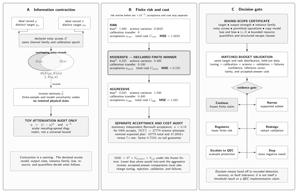
Information contraction, finite bias–variance–cost accounting, and the resulting mitigation decision gate. — A mitigation claim passes three distinct gates: preserve the theorem’s access and output scope, reproduce finite bias–variance–acceptance and total-cost arithmetic, and validate the final decision at matched resources. The attenuation factor $\eta=(1-p)^L$ is a toy diagnostic, not a universal error-mitigation law.

Scaling Bounds and Their Quantifiers

Depth, width, and observable light cones are different resources

Depth $L$ , width $M$ or $n$ , total gate count, and the number of noisy gates in an observable’s backward light cone can scale differently. A layer of parallel gates increases depth once but may expose many qubits; a local observable in a geometrically local circuit may depend on only a small region until its light cone grows. A bound exponential in selected noisy layers is not automatically exponential in every definition of circuit size, and an exponential dependence on width for rapidly scrambling circuits need not describe a fixed-width depth study.

Tsubouchi, Sagawa, and Yoshioka (2023) derive quantum-estimation-theoretic copy bounds for a virtual-circuit class. Its scope certificate fixes an unbiased estimate of a traceless observable with a declared standard deviation; an $n$ -qubit, $L$ -layer circuit with Markovian post-layer channels that are injective and full rank; randomized controls and noise boosting no weaker than the baseline; $N$ noisy-circuit copies; and a joint final POVM. Their generic depth result has a sharper unital case. Their exponential-in-width result is an average statement for random layered circuits with unitary two-design structure; broader brick-wall behavior and biased rescaling beyond the exact global-depolarizing case are numerical evidence, not the same theorem. Error correction is outside their virtual-circuit class.

Worst-case families do not describe every circuit

Quek et al. (2024) obtain substantially tighter lower bounds by constructing hard circuits whose noisy outputs rapidly lose information. Their scope certificate fixes a classical description of the ideal circuit and observables, $m$ copies of the noisy output, arbitrary collective measurement, weak expectation or strong computational-basis sampling output as separately defined, and a copy-count resource. The headline local-depolarizing and non-unital results are worst-case statements; the shortest-depth constructions use rapid mixing and all-to-all connectivity, while geometrically local variants have separately stated depth scalings. The main weak-mitigation bounds also specify whether the algorithm is input-state agnostic, and their input-aware conclusion introduces a classical-algorithm alternative rather than silently retaining the same claim.

Those results can disqualify a universal promise covering the hard family. They cannot be applied merely because an experiment has the same qubit count and nominal error rate. The auditor must match connectivity, circuit ensemble, input knowledge, output class, noise placement, loss, failure probability, and the counted copies. Exact knowledge of the noise is already allowed in parts of the analysis, so “better calibration” does not answer those particular lower bounds; special structure outside the hard family may.

Weak and strong mitigation support different conclusions

Theorem 3 of Takagi, Tajima, and Gu (2023) provides a particularly transparent weak-estimation lower bound when all of its hypotheses are retained. Let $\mathcal S$ be a target-state family containing at least two states, $\mathcal O$ the observable family, $\widehat E_A(\rho)$ the estimate returned for $\operatorname{Tr}(A\rho)$ , $\delta\ge0$ the allowed absolute error, and $0\le\epsilon\le1/2$ the failure probability. The required performance condition is, for every $\rho\in\mathcal S$ and $A\in\mathcal O$ ,

\Pr\!\left( \left|\operatorname{Tr}(A\rho)-\widehat E_A(\rho)\right| \le \delta \right) \ge 1-\epsilon, \qquad D_{\mathcal O}(\rho,\sigma) := \max_{A\in\mathcal O} \left|\operatorname{Tr}\!\left[A(\rho-\sigma)\right]\right|.

Its scope certificate uses only the paper’s $M$ -qubit layered model. Index the $N$ distorted output states by $r$ , the $L$ selected unitary layers by $\ell$ , and the $M$ qubits by $m$ . After each selected unitary layer, at every $(r,\ell,m)$ location, local depolarizing noise

\mathcal D_{\gamma_{r\ell m}}(\tau) =(1-\gamma_{r\ell m})\tau +\gamma_{r\ell m}\frac{I}{2}

has strength $\gamma_{r\ell m}\ge\gamma$ . The intermediate operations from the $M$ -qubit system to itself are unital, and an arbitrary final process receives the $N$ distorted states. Quantum error correction is excluded from this model. If some $\rho,\sigma\in\mathcal S$ satisfy $D_{\mathcal O}(\rho,\sigma)\ge2\delta$ , Theorem 3 gives the necessary condition

N \ge \frac{(1-2\epsilon)^2} {2\ln 2\,M(1-\gamma)^{2L}}.

Every symbol is a theorem resource or performance parameter: $M$ is circuit width, $L$ counts the selected noisy layers, $\gamma$ is a uniform lower bound on every local depolarizing strength, $\delta$ is absolute estimation accuracy, $\epsilon$ is failure probability, and $N$ is the total number of distorted output states or noisy samples supplied to the final mitigation process. $N$ is not the number of rounds, accepted samples, calibration attempts, or wall-clock seconds.

For an exact numerical fixture, take

\delta=0.2,\quad \rho=|0000\rangle\langle0000|,\quad \sigma=|1111\rangle\langle1111|,\quad A=|0000\rangle\langle0000|, \quad D_{\mathcal O}=1\ge 0.4,

where $\mathcal O=\{A\}$ is the singleton observable family. With $M=4$ , $\gamma=0.02$ , $L=200$ , and $\epsilon=0.05$ , the numerator is $(1-2\epsilon)^2=0.9^2=0.81$ , while

0.98^{400}=0.00030933586580571048, \qquad 2\ln 2\,(4)(0.98^{400})=0.0017153222658343825.

Substitution gives

\frac{0.9^2}{0.0017153222658343825} =472.21447312467114, \qquad N\ge 473.

The ceiling is valid because $N$ counts states and must be an integer: every integer satisfying $N\ge472.21447312467114$ is at least $473$ . This is a necessary theorem-scoped condition. It is neither a sufficient budget for achieving the performance guarantee nor an observed-shot prediction. Calibration, rejection, and time would require additional accounting.

Classical computation and input-state knowledge alter the access model

Giving a protocol a full classical description of the input or ideal circuit may enable classical computation that uses no noisy samples. A lower bound on quantum samples alone then cannot rule out an expensive classical solution; it must either charge classical work or state a disjunction between large sample use and an equivalent classical procedure. Conversely, denying the mitigation algorithm input information can strengthen a lower bound but narrows its applicability.

The relevant question is not whether classical computation is “free” in the abstract. It is what the theorem counts and what the application budget permits. A protocol may trade quantum samples for exponential classical post-processing, memory, or exact input-state knowledge. That is a genuine resource conversion, not a contradiction. It must be exposed before the result is called efficient.

Structured Exceptions and Finite Useful Regimes

Shallow, local, symmetric, and problem-specific structure can matter

A finite protocol can be useful when contraction is modest, the relevant observable has a small light cone, the circuit preserves a verified sector, the noise has a stable sparse description, or the task needs only a few bounded expectations. Such structure changes the instance family or target, not the validity of a theorem about a broader hard family. It must be declared before inspecting results and tested on held-out instances.

The original ZNE proposals of Li and Benjamin (2017) and Temme, Bravyi, and Gambetta (2017), the practical combined methods of Endo, Benjamin, and Li (2018), and the broader hybrid review of Endo, Cai, Benjamin, and Yuan (2021) provide constructive finite-regime evidence. Suzuki et al. (2022) discuss mitigation across NISQ and fault-tolerant eras. These works show available strategies and use cases; they do not prove favorable asymptotic scaling for every noise family.

A finite success does not establish favorable asymptotic scaling

A demonstration at a few depths and widths establishes what was measured at those sizes, within reference and selection uncertainty. It does not identify a polynomial or exponential law without a prespecified scaling family, sufficient dynamic range, competing functional forms, and uncertainty on the fit. Fixed total shots can also create a floor that hides the growth of variance until larger sizes.

Finite success should therefore be reported directly: target, device epoch, circuits, estimator, attempted and accepted budget, accuracy, confidence, and comparator. Avoid extrapolating “scalable” from a visually stable short curve. The result remains useful without an asymptotic adjective.

A worst-case lower bound does not erase a validated finite result

Worst-case theorems rule out a uniform low-cost guarantee over a family containing hard instances. They do not say that every member is hard, nor do they retroactively invalidate a well-controlled finite estimate. A validated structured result and a worst-case asymptotic barrier can both be true. The former tells us where the present protocol worked; the latter constrains how broadly that success may be promised.

Wang et al. (2024) study whether error mitigation can improve trainability of noisy variational algorithms and identify regime-dependent limitations. Their trainability analysis is not a universal error-mitigation no-go. It is evidence that the target—optimization signal rather than a single final expectation—and the noise-induced landscape matter. The appropriate frontier statement is conditional: useful finite regimes exist, while transferable scaling claims remain method-, structure-, and resource-dependent.

Benchmark at Matched Accepted-Answer Cost

Compare the same target and task distribution

Every comparator must solve the same frozen problem on the same prespecified task distribution. Raw and mitigated estimates should use the same ideal observable and loss; a classical baseline should receive the same input information; a sampling method should not be compared with an expectation estimator as though their outputs were interchangeable. Match accuracy and confidence, then compare the resources required per accepted answer.

Charge calibration, tuning, rejection, and validation

The headline science-shot count is only one coordinate. Charge noise learning, calibration refreshes, hyperparameter searches, deliberately amplified circuits, rejected records, failed jobs, reference construction, validation, and classical post-processing. Amortization is allowed only over the declared reuse horizon and transfer domain. Algorithmic Benchmarking owns the end-to-end comparison; this page supplies the mitigation-specific disqualification tests.

Selection on favorable circuits invalidates population claims

Selecting circuits after seeing which ones mitigation helps converts a population claim into a selected-subset claim. The repair is to predeclare strata and selection rules, retain all attempted instances, or narrow the conclusion and validate the restricted family independently. A benchmark may still report heterogeneous effects, but the failures and excluded circuits belong beside the successes.

Report failure probability and reference uncertainty

An error bar on $\widehat\mu$ is incomplete if the ideal reference is itself uncertain or if the pipeline can abstain, fail to converge, or return no accepted answer. Report interval construction, coverage target, all failure events, reference uncertainty, and the number of attempts. Export the complete record to Reporting Standards rather than treating a plot legend as reproducibility metadata.

Compose Methods Without Multiplying Licenses

Individually validated components need not form a validated stack

A response correction, physical suppression layer, extrapolator, or sector filter can pass its own test yet fail after composition. Order changes the data distribution and often the estimand. A license proved on raw outputs does not automatically transfer to outputs already conditioned, folded, randomized, or pulse-compiled.

Shared records create covariance and selection dependence

Components may reuse shots, calibration models, randomized circuits, or training data. Such reuse can be efficient, but it does not create independent evidence. Shared records introduce covariance; choosing a downstream estimator after inspecting upstream results introduces selection. Propagate the joint estimator or resample the entire pipeline rather than adding component variances as if independent.

Every upstream intervention changes downstream evidence

A physical intervention changes the channel seen by every later method. Refit or revalidate the downstream model, acceptance rule, weights, covariance, and transfer domain after the intervention. Freeze the full stack before held-out validation. Component certificates are inputs to this record, not licenses that multiply into a system-level guarantee.

Why Mitigation Does Not Replace Fault Tolerance

Output inference is not protected quantum evolution

Mitigation typically returns selected classical estimates after a noisy computation. It need not preserve an unknown logical state through intermediate operations, support adaptive coherent use, or produce a reusable channel. Better final expectations are therefore not evidence that information remained protected throughout the circuit.

Threshold claims require encoded fault containment

A threshold theorem concerns an encoded architecture, a fault model, fault-tolerant gadgets, syndrome extraction, recovery or decoding, and a scaling construction that suppresses logical failure below a threshold. None follows from a finite mitigated observable. Threshold Theorem owns those hypotheses; Why Quantum Error Correction Is Possible owns correctability and encoded recovery.

Mitigation and QEC can coexist without becoming equivalent

Mitigation may improve a finite logical observable, help characterize an encoded experiment, or complement detection and correction. QEC may in turn reduce noise enough that a finite estimator becomes practical. This coexistence changes the combined resource ledger but not the concepts: one infers selected outputs, the other protects encoded information. Escalating to QEC is a decision to evaluate a different architecture, not a claim that a threshold has already been met.

Executable Finite Audits and Stop Decisions

The following fixtures are deliberately small, reproducible calculations. Audits 1, 2, and 4 are finite estimator and cost examples; Audit 3 is a scalar attenuation toy. None is a consequence of the asymptotic theorems above, and none supplies an observed hardware budget.

Audit 1: signed-weight allocation

For weights $(1.5,-0.5)$ , independent per-shot standard deviations $(1,1)$ , and $20{,}000$ science shots, the allocation rule gives $(15{,}000,5{,}000)$ . The variance is $0.0002$ and standard error $0.01414213562373095$ , below equal allocation’s $0.00025$ and $0.015811388300841896$ . This conclusion uses independent strata and the declared variances.

Audit 2: bias–variance–calibration risk

Using $b^2+v/n+v_{\mathrm{cal}}$ , the raw, moderate, and aggressive risks are $0.0016625000000000001$ , $0.0007250000000000001$ , and $0.001925$ ; their RMSEs are $0.04077376607575023$ , $0.02692582403567252$ , and $0.04387482193696061$ . The moderate estimator wins this finite MSE comparison even though the aggressive estimator has smaller bias. This is not a universal ranking of regularizers.

Audit 3: an attenuation-cost toy model

For the explicitly scalar toy $\eta=(1-p)^L$ with $p=0.02$ and $L=100$ , $\eta=0.13261955589475294$ and the rescaling factor in variance is $\eta^{-2}=56.857120527912684$ . Multiplying an ideal standard-error budget of $10{,}000$ shots by this factor and taking a ceiling gives $568{,}572$ . This is not a theorem about arbitrary circuits, observables, noise, or mitigation protocols.

Audit 4: acceptance and unconditional cost

With acceptance $a=0.18$ and conditional mean $0.72$ , the subnormalized mean is $0.1296$ . Under stationary independent Bernoulli acceptance, the stopping time $T$ needed to collect $5{,}000$ accepted science records has $\mathbb E[T]=5{,}000/0.18$ ; the integer planning conversion is $\lceil\mathbb E[T]\rceil=27{,}778$ , not a guarantee that a fixed run of $27{,}778$ attempts succeeds. Adding $6{,}000$ calibration attempts gives the nominal expected planning total $33{,}778$ . At $0.0014$ seconds per attempt, its nominal expected planning time is $47.2892$ seconds rather than the raw accepted-record time of $7$ seconds, a ratio of $6.7556$ . A guaranteed or high-confidence budget for obtaining the accepted count requires a binomial or stopping-time tail calculation. Neither conditional nor subnormalized mean is the original ideal target without an additional argument.

// LIMITS_OF_ERROR_MITIGATION_FINITE_AUDITS
import assert from 'node:assert/strict';

const close = (actual, expected, tolerance = 1e-15) => {
  assert.ok(
    Math.abs(actual - expected) <= tolerance,
    `expected ${expected}, received ${actual}`,
  );
};

// Audit 1: signed-weight allocation.
const weights = [1.5, -0.5];
const perShotSigma = [1, 1];
const scienceBudget = 20_000;
const coefficientOneNorm = weights.reduce(
  (sum, weight) => sum + Math.abs(weight),
  0,
);
const allocationDenominator = weights.reduce(
  (sum, weight, index) =>
    sum + Math.abs(weight) * perShotSigma[index],
  0,
);
const optimalAllocation = weights.map((weight, index) =>
  scienceBudget *
  Math.abs(weight) *
  perShotSigma[index] /
  allocationDenominator
);
const independentVariance = (allocation) =>
  weights.reduce(
    (sum, weight, index) =>
      sum +
      weight ** 2 *
      perShotSigma[index] ** 2 /
      allocation[index],
    0,
  );
const optimalVariance = independentVariance(optimalAllocation);
const equalAllocation = [10_000, 10_000];
const equalVariance = independentVariance(equalAllocation);

assert.equal(coefficientOneNorm, 2);
assert.equal(coefficientOneNorm ** 2, 4);
assert.deepEqual(optimalAllocation, [15_000, 5_000]);
close(optimalVariance, 0.0002);
close(Math.sqrt(optimalVariance), 0.01414213562373095);
close(equalVariance, 0.00025);
close(Math.sqrt(equalVariance), 0.015811388300841896);
assert.ok(optimalVariance < equalVariance);

// Audit 2: bias–variance–calibration risk.
const risk = ({ bias, perShotVariance, shots, calibrationVariance = 0 }) =>
  bias ** 2 + perShotVariance / shots + calibrationVariance;

const rawRisk = risk({
  bias: 0.04,
  perShotVariance: 0.75,
  shots: 12_000,
});
const moderateRisk = risk({
  bias: 0.015,
  perShotVariance: 3.2,
  shots: 8_000,
  calibrationVariance: 0.0001,
});
const aggressiveRisk = risk({
  bias: 0.005,
  perShotVariance: 12,
  shots: 8_000,
  calibrationVariance: 0.0004,
});

close(rawRisk, 0.0016625000000000001);
close(Math.sqrt(rawRisk), 0.04077376607575023);
close(moderateRisk, 0.0007250000000000001);
close(Math.sqrt(moderateRisk), 0.02692582403567252);
close(aggressiveRisk, 0.001925);
close(Math.sqrt(aggressiveRisk), 0.04387482193696061);
assert.ok(moderateRisk < rawRisk);
assert.ok(moderateRisk < aggressiveRisk);
assert.ok(0.005 < 0.015);

// Audit 3: attenuation-cost toy model.
const perLayerAttenuation = 1 - 0.02;
const layers = 100;
const attenuation = perLayerAttenuation ** layers;
const rescalingOverhead = attenuation ** -2;
const targetStandardError = 0.01;
const idealShots = targetStandardError ** -2;
const rescaledShots = Math.ceil(idealShots * rescalingOverhead);

close(attenuation, 0.13261955589475294);
close(rescalingOverhead, 56.857120527912684, 1e-13);
assert.equal(idealShots, 10_000);
assert.equal(rescaledShots, 568_572);

// Audit 4: acceptance and unconditional cost.
const acceptance = 0.18;
const conditionalMean = 0.72;
const unconditionalMean = acceptance * conditionalMean;
const requiredAccepted = 5_000;
const scienceAttempts = Math.ceil(requiredAccepted / acceptance);
const calibrationAttempts = 6_000;
const totalAttempts = scienceAttempts + calibrationAttempts;
const secondsPerAttempt = 0.0014;
const totalSeconds = totalAttempts * secondsPerAttempt;
const rawSeconds = requiredAccepted * secondsPerAttempt;

close(unconditionalMean, 0.1296);
assert.equal(scienceAttempts, 27_778);
assert.equal(totalAttempts, 33_778);
close(totalSeconds, 47.2892);
close(rawSeconds, 7);
close(totalSeconds / rawSeconds, 6.7556);

console.log('Limits-of-error-mitigation finite audits: PASS');

Continue, narrow, regularize, redesign, escalate, or stop

The decision must follow the evidence gate that failed or passed. “Continue” means only that held-out benefit remains positive for the frozen finite claim at matched cost and confidence. “Escalate” means that the mitigation-only route cannot meet the declared need and that encoded options should be evaluated; it is not itself a threshold result. Store enough evidence to reproduce the decision and define what future evidence could reverse it.

Decision	Evidence threshold	Trigger	Retained claim	Next permitted action	Stored evidence
Continue	held-out benefit remains positive at matched total cost and declared confidence	model, calibration, acceptance, and reference checks pass	finite claim for the frozen task and regime	collect the prespecified final data	complete scope certificate and validation record
Narrow	only a subset of observables, circuits, depths, contexts, or epochs transfers	population or context check fails outside a supported subset	explicitly restricted finite claim	rerun independent validation on the restricted set	excluded strata and revised quantifiers
Regularize	lower-bias inversion loses on MSE or stability	variance, calibration sensitivity, or conditioning dominates	biased but lower-risk estimator under the declared loss	freeze regularization before final validation	bias, variance, calibration, and selection ledger
Redesign	target, access, or implementation does not satisfy the selected protocol license	residual, drift, composition, or feasibility test fails	no performance claim for the rejected design	change protocol or physical experiment and restart validation	failure trace and changed-design boundary
Escalate	required accuracy, output strength, or duration cannot be reached at accepted cost	finite stress test or scoped bound rules out the mitigation-only route	local stop decision, not a universal impossibility theorem	evaluate encoded detection, recovery, or fault tolerance	explicit handoff to the QEC owner
Stop	no supported finite regime remains or evidence cannot identify benefit	matched-budget comparison, identifiability, or independent validation fails	documented negative result within frozen scope	archive the claim and define an update trigger	full negative-result record and reproduction assets

Exercises

Allocate a Signed Estimator

For $w=(1.5,-0.5)$ , $\sigma=(1,1)$ , and $N=20{,}000$ , derive the independent-stratum optimum and compare it with equal allocation.

Solution

Minimize $\sum_j w_j^2\sigma_j^2/n_j$ subject to $\sum_jn_j=N$ . The Lagrange equations give $n_j\propto|w_j|\sigma_j$ , hence $(n_1,n_2)=(15{,}000,5{,}000)$ . The variance is $2.0\times10^{-4}$ and standard error is $0.01414213562373095$ . Equal allocation gives variance $2.5\times10^{-4}$ and standard error $0.015811388300841896$ . Shared records or calibration create covariance, so the independent sum and this allocation cease to be valid.

Convert Standard Error to Tail Confidence

For $\Gamma=2$ , $\epsilon=0.02$ , and $\delta=0.05$ , apply the stated Hoeffding condition.

Solution

Substitution gives

\left\lceil \frac{2(2^2)}{(0.02)^2}\ln(40) \right\rceil =73{,}778.

This is sufficient under independent draws and the bound $Z\in[-2,2]$ . It is not the exact sample complexity, a standard-error conversion, or an information-theoretic lower bound; a tighter distribution-specific analysis could require fewer samples.

Choose by MSE Rather Than Bias Alone

Reconstruct Audit 2 and choose the estimator under squared-error loss.

Solution

The raw, moderate, and aggressive MSEs are respectively $0.0016625000000000001$ , $0.0007250000000000001$ , and $0.001925$ . Their RMSEs are $0.04077376607575023$ , $0.02692582403567252$ , and $0.04387482193696061$ . Choose the moderate estimator. The aggressive estimator’s bias, $0.005$ , is smaller than $0.015$ , but its science variance and calibration-transfer variance more than erase that advantage.

Scope an Exponential Lower Bound

Audit a proposed application of a layered local-depolarizing lower bound.

Solution

Record the ideal target, weak or strong output, circuit family, depth, width, locality, observable family, local noise placement and strength, permitted operations, copy model, input knowledge, bias or loss, accuracy, confidence, counted resource, and worst- or average-case quantifiers. Only then match the instance. “All mitigation is exponentially costly” drops these restrictions. “One finite success refutes the theorem” also fails: a structured finite instance can lie outside the hard family or below the asymptotic regime.

Audit Conditional Acceptance

Reconstruct Audit 4 and distinguish its three possible targets.

Solution

For stationary independent Bernoulli acceptance, the stopping time obeys $\mathbb E[T]=5000/0.18$ , so $\lceil\mathbb E[T]\rceil=27{,}778$ is an integer expected-planning conversion, not a fixed-attempt guarantee. Calibration raises the nominal expected planning total to $33{,}778$ . The conditional mean is $0.72$ ; the subnormalized mean is $0.18(0.72)=0.1296$ . Nominal expected planning time is $33{,}778(0.0014)=47.2892$ seconds, versus $7$ seconds for $5{,}000$ raw records, a ratio $6.7556$ . A guaranteed or high-confidence accepted-count budget needs a tail calculation. Neither mean equals the original ideal target without a target-preservation argument.

Design a Matched-Budget Benchmark

Specify a fair benchmark for a raw estimator and two mitigation pipelines.

Solution

Freeze one ideal target, task distribution, loss, accuracy, and confidence. Give every comparator the same declared resource vector and charge tuning, calibration, science attempts, rejection, failed jobs, validation, classical work, and uncertain reference construction. Predeclare circuit strata and the selection rule; do not inspect results and retain only favorable circuits. Compare cost per accepted answer and report failures as outcomes rather than deleting them.

Test a Composed Mitigation Stack

Audit one physical intervention followed by two estimator-level methods.

Solution

Use the dependency order physical intervention $\to$ first estimator $\to$ second estimator. The intervention changes the downstream channel; the first estimator changes the records and possibly the target seen by the second. Shared shots or calibration induce covariance, while choosing the second method after inspecting the first creates selection dependence. Refit downstream model records after the intervention and require fresh held-out validation of the frozen complete stack.

Write an Escalation Record

Turn a failed mitigation audit into a bounded scientific decision.

Solution

Choose exactly the supported action: continue, narrow, regularize, redesign, escalate, or stop. Preserve any validated finite claim—for example, benefit for specified local observables and depths—while naming the failed gate, such as acceptance-adjusted cost or model transfer. Escalation means evaluating encoded detection, recovery, or fault tolerance because mitigation cannot meet the frozen requirement. It does not assert that a code threshold is satisfied or that a fault-tolerant implementation exists.

References

Daniel Bultrini, Max Hunter Gordon, Piotr Czarnik, Andrew Arrasmith, M. Cerezo, Patrick J. Coles, and Lukasz Cincio, “Unifying and benchmarking state-of-the-art quantum error mitigation techniques,” Quantum 7, 1034 (2023), doi:10.22331/q-2023-06-06-1034.
Zhenyu Cai, Ryan Babbush, Simon C. Benjamin, Suguru Endo, William J. Huggins, Ying Li, Jarrod R. McClean, and Thomas E. O’Brien, “Quantum error mitigation,” Reviews of Modern Physics 95, 045005 (2023), doi:10.1103/RevModPhys.95.045005.
Suguru Endo, Simon C. Benjamin, and Ying Li, “Practical Quantum Error Mitigation for Near-Future Applications,” Physical Review X 8, 031027 (2018), doi:10.1103/PhysRevX.8.031027.
Suguru Endo, Zhenyu Cai, Simon C. Benjamin, and Xiao Yuan, “Hybrid Quantum-Classical Algorithms and Quantum Error Mitigation,” Journal of the Physical Society of Japan 90, 032001 (2021), doi:10.7566/JPSJ.90.032001.
Ying Li and Simon C. Benjamin, “Efficient Variational Quantum Simulator Incorporating Active Error Minimization,” Physical Review X 7, 021050 (2017), doi:10.1103/PhysRevX.7.021050.
Angus Lowe, Max Hunter Gordon, Piotr Czarnik, Andrew Arrasmith, Patrick J. Coles, and Lukasz Cincio, “Unified approach to data-driven quantum error mitigation,” Physical Review Research 3, 033098 (2021), doi:10.1103/PhysRevResearch.3.033098.
Yihui Quek, Daniel Stilck França, Sumeet Khatri, Johannes Jakob Meyer, and Jens Eisert, “Exponentially tighter bounds on limitations of quantum error mitigation,” Nature Physics 20, 1648–1658 (2024), doi:10.1038/s41567-024-02536-7.
Dayue Qin, Yanzhu Chen, and Ying Li, “Error statistics and scalability of quantum error mitigation formulas,” npj Quantum Information 9, 35 (2023), doi:10.1038/s41534-023-00707-7.
Yasunari Suzuki, Suguru Endo, Keisuke Fujii, and Yuuki Tokunaga, “Quantum Error Mitigation as a Universal Error Reduction Technique: Applications from the NISQ to the Fault-Tolerant Quantum Computing Eras,” PRX Quantum 3, 010345 (2022), doi:10.1103/PRXQuantum.3.010345.
Ryuji Takagi, “Optimal resource cost for error mitigation,” Physical Review Research 3, 033178 (2021), doi:10.1103/PhysRevResearch.3.033178.
Ryuji Takagi, Suguru Endo, Shintaro Minagawa, and Mile Gu, “Fundamental limits of quantum error mitigation,” npj Quantum Information 8, 114 (2022), doi:10.1038/s41534-022-00618-z.
Ryuji Takagi, Hiroyasu Tajima, and Mile Gu, “Universal Sampling Lower Bounds for Quantum Error Mitigation,” Physical Review Letters 131, 210602 (2023), doi:10.1103/PhysRevLett.131.210602.
Kristan Temme, Sergey Bravyi, and Jay M. Gambetta, “Error Mitigation for Short-Depth Quantum Circuits,” Physical Review Letters 119, 180509 (2017), doi:10.1103/PhysRevLett.119.180509.
Kento Tsubouchi, Takahiro Sagawa, and Nobuyuki Yoshioka, “Universal Cost Bound of Quantum Error Mitigation Based on Quantum Estimation Theory,” Physical Review Letters 131, 210601 (2023), doi:10.1103/PhysRevLett.131.210601.
Ewout van den Berg, Zlatko K. Minev, Abhinav Kandala, and Kristan Temme, “Probabilistic error cancellation with sparse Pauli–Lindblad models on noisy quantum processors,” Nature Physics 19, 1116–1121 (2023), doi:10.1038/s41567-023-02042-2.
Samson Wang, Piotr Czarnik, Andrew Arrasmith, M. Cerezo, Lukasz Cincio, and Patrick J. Coles, “Can Error Mitigation Improve Trainability of Noisy Variational Quantum Algorithms?” Quantum 8, 1287 (2024), doi:10.22331/q-2024-03-14-1287.