Measurement Error Mitigation

Measurement error mitigation treats terminal readout as a calibrated inverse problem. A latent outcome $z$ in a declared alphabet is transformed into a reported outcome $y$ by a classical response, and finite calibration and science records support an estimate of a latent distribution or diagonal observable. The result can be a better estimator when the response is identifiable, stable enough, and validated in the science context. It is not a repaired detector, restored quantum state, or corrected circuit trajectory. This page fixes the response orientation, separates detector response from empirical confusion, compares inverse and forward procedures, propagates science and calibration uncertainty, and makes structural assumptions, drift, acceptance, and total cost part of the claim.

Required background. SPAM Errors supplies the assignment license, preparation–measurement nonidentifiability, outcome and context conventions, and transfer boundary needed before a response is inverted. Error Mitigation Overview supplies the frozen estimand, estimator, validation split, and total-resource record.

Helpful background. Quantum Measurement as Estimation supplies likelihood, loss, identifiability, and coverage language, while Variance and Covariance supplies multinomial and shared-calibration covariance propagation.

Measurement Mitigation Is a Calibrated Inverse Problem

Correction changes an estimator, not a detector

A measurement-response experiment yields classical records. Mitigation applies a declared transformation to those records, together with calibration information, to estimate a quantity that would have been obtained from a licensed latent alphabet. It may reduce bias in a population, parity, or diagonal expectation, yet it does not alter the detector that produced the records. Nor does it imply that a density operator existed whose complete statistics equal all independently corrected observables.

This distinction keeps the scientific claim proportional to the evidence. An inverse can assign signed weights to reported outcomes; a constrained reconstruction can move an estimate to the probability simplex; an observable-specific method can avoid reconstructing a global distribution. These are different estimators with different sampling laws. The review by Cai et al. (2023) places readout correction inside the broader error-mitigation landscape, where assumptions, calibration, variance, and resource overhead qualify every improvement claim.

The terminal classical-response license

The response model begins after a SPAM analysis has named the latent and reported alphabets, preparation trust, context, epoch, and acquisition order. Its narrow license says that, for the terminal measurement and workload under study, a column-stochastic classical map relates latent probabilities to reported probabilities. It does not identify a POVM, quantum instrument, analog detector mechanism, or conditional postmeasurement state. Maciejewski, Zimborás, and Oszmaniec (2020) derive correction from detector tomography under trusted-probe assumptions; that route is stronger than fitting a command-to-report table and therefore must not be inferred from such a table alone.

The license also fixes transfer. A response calibrated on isolated basis preparations may fail under simultaneous readout, changed schedules or classifiers, leakage, or later epochs. Retain its data and version, test representative holdouts, and expire it when transfer or drift fails.

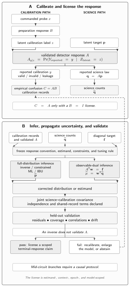
Terminal measurement mitigation is a calibrated inverse problem. The empirical table $C=AB$ separates preparation response from detector response, while full-distribution or observable-dual inference propagates science and calibration uncertainty through held-out residual, correlation, coverage, and drift checks. Failed validation licenses recalibration, model enlargement, or abstention—not a repaired detector, restored state, or corrected mid-circuit trajectory.

What this specialist page owns

The specialist calculation starts with calibrated counts and ends with a scoped terminal estimate. It owns the orientation of response matrices; the distinction among preparation, detector, and empirical command-to-report maps; algebraic identifiability and finite sensitivity; inverse, constrained, likelihood, unfolding, regularized, and observable-dual procedures; structured multiqubit models; propagation of both science and calibration randomness; and held-out tests of correlation, context transfer, and drift. Bravyi et al. (2021) and Geller (2021) show how useful multiqubit correction claims depend on explicit structural and SPAM-qualified assumptions rather than on the phrase “measurement correction” alone.

It does not allocate preparation versus measurement error, reconstruct a POVM, instrument, state, or process, engineer detectors, choose all mitigation families, run calibration services, benchmark applications, restore logical information, or establish fault tolerance. Those tasks require different evidence and owners.

Fix the Response Convention and the Estimand

Reported outcomes are rows and latent outcomes are columns

Let $Z_{\mathrm{latent}}$ denote the outcome that would be available immediately before the licensed terminal classical response, and let $Y_{\mathrm{reported}}$ denote the stored report. Adopt

$$A_{y|z} = \Pr(Y_{\mathrm{reported}}=y\mid Z_{\mathrm{latent}}=z), \qquad \sum_y A_{y|z}=1, \qquad \mathbf q=A\mathbf p.$$

Thus reported outcomes $y$ are rows, latent outcomes $z$ are columns, $\mathbf p$ is the latent distribution, and $\mathbf q$ is the reported distribution. Every column is stochastic because it conditions on one latent event. Writing the conditional probability before displaying a matrix prevents the common transpose error.

For a binary response define

$$A = \begin{pmatrix} 1-\alpha & \beta\\ \alpha & 1-\beta \end{pmatrix}, \qquad d=1-\alpha-\beta.$$

Here $\alpha=\Pr(1|0)$ and $\beta=\Pr(0|1)$. If $m=p_0-p_1$ and $m_{\mathrm{obs}}=q_0-q_1$, direct substitution gives

$$m_{\mathrm{obs}} = (\beta-\alpha)+d\,m, \qquad m = \frac{m_{\mathrm{obs}}-(\beta-\alpha)}{d}.$$

The inverse exists only when $d\ne0$. The offset $\beta-\alpha$ is essential for asymmetric errors; omitting it or transposing $A$ changes the answer. At $d=0$, both latent columns coincide, so no number of terminal reports distinguishes the two latent probabilities.

Separate A from the observed calibration table C

Calibration hardware normally issues a command $x$ rather than directly preparing a certified latent label $z$. Write the preparation response and empirical confusion table as

$$B_{z|x} = \Pr(Z_{\mathrm{latent}}=z\mid X_{\mathrm{commanded}}=x), \qquad C_{y|x} = \sum_z A_{y|z}B_{z|x}, \qquad C=AB.$$

The calibration frequencies identify $C$, subject to finite sampling and the declared context. They identify detector response $A$ only when an additional preparation license is supplied. Aligned command and latent alphabets with $B=I$ give $C=A$. If $B$ is separately characterized, recovery of $A$ requires the map $A\mapsto AB$ to be injective on the chosen response family—for example, full row rank of $B$ in the unconstrained finite model—and the uncertainty of $B$ must be propagated.

Bounds on preparation response yield a set of compatible detector responses rather than a unique matrix. Alternatively, one may deliberately define a command-relative target and use $C$ as its forward map. That is coherent, but it does not turn $C$ into detector-only $A$. More calibration repetitions shrink uncertainty around $C$; they cannot factor $C=AB$ without new trust or experimental variation. This is the preparation–measurement nonidentifiability retained from the SPAM boundary.

Define the estimand before reconstructing a histogram

The target may be the full latent distribution $\mathbf p$, a marginal, a parity, a diagonal expectation $\mu=\mathbf f^{\mathsf T}\mathbf p$, an accepted conditional distribution, or a decision derived from one of these. These targets need not demand the same response information. Reconstructing $2^n$ probabilities to estimate one local diagonal observable can add calibration and variance costs without adding relevant evidence.

Freeze the target alphabet and order, context and epoch, accepted sectors, loss and utility, uncertainty and coverage threshold, model-comparison rule, validation set, and resource boundary. If a target is conditional on acceptance, report both its definition and the acceptance probability. If the requested quantity is nonlinear in $\mathbf p$, state that nonlinearity before selecting an estimator; a linear inverse followed by an undeclared nonlinear transformation has a different sampling law.

Keep outcome and bitstring order explicit

Write one explicit index map from physical bit labels to stored strings before any matrix is assembled. State whether the order is $00,01,10,11$ or another convention, whether strings are displayed most-significant-bit first, how classical-register order relates to physical wires, and which row and column correspond to each event. The same mapping must be used by calibration, science acquisition, bit-flip masks, marginalization, and reported results.

Invalid classifier codes, timeouts, erasures, loss flags, and resolved leakage reports remain explicit outcomes unless a predeclared coarse graining merges them. A response column that silently drops such events becomes substochastic. Renormalizing it changes the target to a conditional distribution and hides yield. Acquisition order also belongs in the record because a blockwise drift can mimic command dependence or change the response between calibration and science.

Object	Definition	Normalization	Learned from	Licenses	Does not license
$\mathbf p$	Latent terminal distribution	$\mathbf1^{\mathsf T}\mathbf p=1$ on the declared alphabet	Scientific target or model	Latent populations for that target	A prepared quantum state
$\mathbf q$	Reported terminal distribution $A\mathbf p$	$\mathbf1^{\mathsf T}\mathbf q=1$ with all reports retained	Science counts	Report frequencies in context	Latent populations without $A$
$A$	Detector response $A_{y\mid{}z}$	Each latent column sums to one	Trusted latent probes or licensed factorization	Terminal classical forward prediction	A POVM, instrument, or mechanism
$B$	Preparation response $B_{z\mid{}x}$	Each command column sums to one	Independent preparation evidence	Command-to-latent prediction	Detector attribution
$C=AB$	Empirical confusion $C_{y\mid{}x}$	Each command column sums to one	Commanded calibration counts	Command-to-report prediction	$C=A$ without a $B=I$ license
Accepted conditional distribution	$q_y\mathbf1_{\mathcal A}(y)/\Pr(\mathcal A)$	Sums to one over accepted reports	Accepted counts plus total attempts	Conditional reported target	Original unconditional distribution
Diagonal estimand $\mathbf f$ and dual $\mathbf w$	$\mu=\mathbf f^{\mathsf T}\mathbf p$, $A^{\mathsf T}\mathbf w=\mathbf f$	No probability normalization for $\mathbf w$	Target plus validated $A$	Observable-specific correction	Full-histogram recovery

Calibrate a Response That Can Be Identified

Trusted preparations and the meaning of calibration

A calibration column is a multinomial experiment conditioned on a preparation claim. To interpret it as a column of $A$, the latent preparation must be trusted, separately bounded, or included in a joint model whose unresolved freedoms are reported. Basis commands alone do not provide this trust. Calibration metadata should record preparation protocol, reset history, spectators, simultaneous operations, measurement settings, classifier version, timestamps, accepted outcomes, and the number of trials per column.

When $B=I$ is only approximate, sensitivity analysis should vary plausible $B$ within its uncertainty or identified set. If the resulting corrected quantity changes materially, preparation uncertainty is part of the dominant error budget. Geller’s conditionally rigorous transition-matrix approach makes this dependency explicit: rigor is conditional on assumptions that suppress or bound the relevant state-preparation contribution and on a response model that transfers.

Full matrices, product factors, and local models

For $n$ binary outcomes, a full response has $2^n$ columns and $2^n-1$ free probabilities in each column, hence $2^n(2^n-1)$ free parameters. It normally requires every computational-basis preparation and sufficient records to resolve rare outcomes. This model can represent arbitrary classical correlations inside the declared alphabet, but its calibration and storage costs become exponential.

A product response assumes

$$A_{\mathbf y|\mathbf z} = \prod_{j=1}^{n}A^{(j)}_{y_j|z_j},$$

reducing the parameter count to $2n$ for binary columns. This is a physical hypothesis of conditional independence and locality, not a numerical convenience that becomes true at large $n$. Local or context-conditioned factors may include neighbor states, simultaneous-readout groups, or a sparse graphical dependence. The declared structure determines which calibration preparations and falsifiers are required.

Correlated responses require correlated tests

One-bit error rates are marginals of a joint response. They do not determine whether flips occur independently, in pairs, or through larger correlated patterns. Two responses can have identical error probability on every bit while assigning very different probability to parity and multibit events. Validation must therefore include joint residuals suited to the intended observables: pair and cluster correlations, parity sectors, Hamming-weight tails, conditional spectator behavior, or direct workload loss.

A product model should be compared against at least one richer alternative on held-out preparations. Residuals must retain sign and outcome structure rather than collapse immediately to average assignment fidelity. For a science target dominated by rare outputs, calibration should deliberately probe those outputs; an excellent average fit can coexist with a severe error in the relevant tail.

Retain contexts, epochs, and acquisition order

Attach a context label and epoch to every response estimate. Context includes measured subset, spectator preparation, concurrent drives and readout, compilation and pulse versions, detector settings, classifier, reset mode, temperature or other retained environment data, and acceptance rules. An epoch should be short enough that stationarity is plausible and long enough to estimate the response; this compromise must be checked empirically.

Preserve order and timestamps. Interleaved sentinels can reveal drift, hysteresis, or shot history. Bracketing science with calibrations supports interpolation only under a justified time model, and pooling epochs requires exchangeability.

The model record includes a validity window and expiry condition even when no drift is detected. Proctor et al. (2020) show how processor drift can be detected and tracked statistically; chronology is therefore part of validation rather than an informal note.

Test Rank and Conditioning Before Solving

Rank controls algebraic identifiability

For full-distribution recovery, distinct latent distributions must produce distinct reported distributions inside the declared model. Algebraically, the relevant columns of $A$ need full rank. If the rank is deficient, a nonzero vector $\mathbf v$ satisfies $A\mathbf v=0$, so $\mathbf p$ and $\mathbf p+t\mathbf v$ are observationally indistinguishable whenever both remain feasible. More science shots cannot separate them.

The Moore–Penrose pseudoinverse then recovers only the component in the identifiable subspace selected by its criterion. A particular regularizer may choose one point among many compatible distributions, but that point is not identified by the records alone. Observable-specific recovery can still be possible: $\mu=\mathbf f^{\mathsf T}\mathbf p$ is identifiable exactly when $\mathbf f$ lies in the range of $A^{\mathsf T}$.

Rectangular responses are legitimate. A tall response can retain erasure or leakage and still have full column rank; a wide response needs structure for full recovery, though selected observables or bounds may survive.

Singular values control finite sensitivity

For a full-rank matrix, singular values quantify how reported perturbations are amplified by inversion. With

$$\kappa_2(A) = \frac{\sigma_{\max}(A)}{\sigma_{\min}(A)},$$

a small $\sigma_{\min}$ marks a direction in latent space that produces little change in reported probabilities. Sampling noise, calibration uncertainty, roundoff, or small model perturbations along that direction can become large after inversion. Report the singular spectrum relevant to the chosen subspace, not only a determinant or a scalar average error.

Conditioning is target-dependent: a global inverse may be unstable while a local dual is stable. Singular-value truncation can help, but its threshold and discarded subspace define a biased estimator.

Model mismatch is not conditioning

Condition number answers a sensitivity question under the assumed matrix. It does not answer whether that matrix describes the science experiment. The identity has perfect condition number and can still be a disastrously wrong response. Conversely, a correctly specified but ill-conditioned response can transfer well while producing large uncertainty. These are distinct failure modes and need distinct diagnostics.

Use rank and singular values before solving, then use calibration-fit residuals, held-out predictive residuals, correlation tests, chronology, and coverage to evaluate adequacy. A physical simplex output, a small optimization residual, or agreement with the fitted calibration table cannot replace held-out evidence. When mismatch dominates, changing the solver treats the symptom; the model must be enlarged, recalibrated, bounded, or rejected.

Choose an Inference Procedure

Direct inverse and pseudoinverse baselines

When $A$ is square and nonsingular, the direct baseline is

$$\widehat{\mathbf p}_{\mathrm{inv}} = A^{-1}\widehat{\mathbf q}.$$

Under an exactly known, correct, stationary response it is linear and unbiased. Its visible weights and amplified directions make it a useful diagnostic, while a large inverse can make finite variance prohibitive.

A negative component is not a negative physical probability. It signals that the empirical reported vector lies outside the image of the probability simplex under the fitted response, or that finite variation has been amplified. Possible causes include ordinary shot noise, calibration noise, drift, structural mismatch, or severe conditioning. Report the signed result and its uncertainty as a diagnostic. Clipping negative values and renormalizing is a new nonlinear estimator; it must be named, tuned, and validated rather than presented as the inverse.

For rectangular or deficient systems, a pseudoinverse or matrix-free solve selects a stated identifiable projection, never information in a null direction. Record tolerance and preconditioner.

Constrained least squares preserves the simplex

With a frozen positive weighting matrix $W$, simplex-constrained weighted least squares is

$$\widehat{\mathbf p}_{\mathrm{CLS}} = \underset{\mathbf p\ge0,\ \mathbf1^{\mathsf T}\mathbf p=1} {\operatorname{arg\,min}} (\widehat{\mathbf q}-A\mathbf p)^{\mathsf T} W (\widehat{\mathbf q}-A\mathbf p).$$

The constraints guarantee a normalized nonnegative output, which is useful when a full distribution is the declared estimand. They also change the estimator. Near a simplex boundary the sampling distribution is asymmetric, standard unconstrained covariance formulas can fail, and projection can introduce finite-sample bias. Choice of $W$ determines which reported residuals matter; estimating $W$ from the same records can add further dependence.

A feasible solution does not validate the response. In Audit 2 constrained least squares returns the nearest boundary, while its nonzero forward residual exposes model failure.

Forward likelihood handles counts directly

For terminal multinomial counts $n_y$, fit the forward model through

$$\widehat{\mathbf p}_{\mathrm{ML}} = \underset{\mathbf p\ge0,\ \mathbf1^{\mathsf T}\mathbf p=1} {\operatorname{arg\,max}} \sum_y n_y\log(A\mathbf p)_y.$$

This uses the count likelihood rather than a Gaussian approximation and naturally respects heteroscedastic multinomial variation. State how terms with $n_y=0$ are handled, forbid positive counts at zero modeled probability, and record constraints, optimizer tolerance, convergence tests, and any boundary solution. If $A$ is uncertain, a joint or hierarchical likelihood can fit its calibration columns rather than pretending they are fixed.

Likelihood chooses the best member of the proposed family; residual and held-out checks must certify the family. Audit 2’s likelihood and constrained fits agree only because the frequency lies beyond the feasible interval.

Iterative Bayesian unfolding and early stopping

Iterative Bayesian unfolding (IBU) applies a multiplicative update. For normalized $\widehat{\mathbf q}$, a simplex initial iterate $\mathbf p^{(0)}$, and positive modeled denominators wherever $\widehat q_y>0$, define

$$p_z^{(k+1)} = p_z^{(k)} \sum_y A_{y|z} \frac{\widehat q_y} {\sum_{z'}A_{y|z'}p_{z'}^{(k)}}.$$

A term with $\widehat q_y=0$ and a zero denominator is assigned its continuous zero-weight limit. In the stated domain, column stochasticity preserves normalization, and nonnegative inputs preserve nonnegativity. Every latent component that might be needed must start with positive mass because the multiplicative rule cannot revive a zero component.

D’Agostini (1995) introduced this unfolding construction; Nachman et al. (2020), Nguyen (2023), and Pokharel et al. (2024) develop quantum-readout, information-theoretic, and scalable IBU treatments. A finite iterate remains start- and stop-dependent, is not automatically a posterior, and still needs calibration uncertainty and transfer tests.

Early stopping suppresses unstable directions before full convergence and therefore acts as implicit regularization. Freeze its criterion on training or tuning data. Inspecting the final holdout to choose the number of steps converts that holdout into tuning data and invalidates the nominal test claim.

Regularization creates a bias–variance choice

Penalties, truncation, shrinkage, smoothing, projection, and early stopping trade sensitivity against bias. State the objective, hyperparameter, constraints, initialization, tolerance, and loss; “stabilized inversion” is not reproducible.

Choose hyperparameters for the declared science targets, because a penalty that improves global error can worsen a rare probability or parity. Compare procedures on representative validation records and freeze the choice before final science.

Procedure	Equation or objective	Output	Simplex guaranteed	Tuning	Principal advantage	Principal failure
Direct inverse	$A^{-1}\widehat{\mathbf q}$	Signed full vector	No	None beyond solver tolerance	Transparent linear baseline	Amplifies noise and mismatch
Pseudoinverse/matrix-free linear solve	Minimum-norm or iterative solution	Identifiable projection	No	Rank cutoff or tolerance	Handles large or rectangular systems	Null directions remain unidentified
Simplex-constrained WLS	Minimize weighted forward residual	Full probability vector	Yes	$W$ and optimizer choices	Enforces physical probabilities	Boundary bias; fit is not validation
Forward multinomial ML	Maximize count log likelihood	Full probability vector	Yes	Optimizer, tolerance, and convergence checks	Uses counts directly	Misspecified response still fits
Explicit penalized/regularized reconstruction	Likelihood or loss plus penalty	Target-dependent estimate	Only if constrained	Penalty and strength	Controls unstable directions	Adds tuning-dependent bias
IBU	Stopped multiplicative update	Full probability vector	Yes in its stated domain	Initial iterate and stopping	Matrix operations preserve positivity	Finite result depends on start and stop
Observable-specific dual	Solve $A^{\mathsf T}\mathbf w=\mathbf f$	One diagonal estimand	Not applicable	Dual-selection criterion	Avoids unnecessary histogram recovery	Weight variance and target-limited scope

Correct the Observable Instead of the Full Histogram

Solve the dual response equation

Suppose the target is the diagonal observable

$$\mu = \mathbf f^{\mathsf T}\mathbf p.$$

If a weight vector satisfies

$$A^{\mathsf T}\mathbf w=\mathbf f,$$

then the sample mean of $w_y$ over reported outcomes is unbiased under a known correct response:

$$\widehat\mu = \mathbf w^{\mathsf T}\widehat{\mathbf q}, \qquad \mathbb E(\widehat\mu) = \mathbf w^{\mathsf T}A\mathbf p = \mathbf f^{\mathsf T}\mathbf p.$$

A solution exists exactly when $\mathbf f$ lies in $\operatorname{range}(A^{\mathsf T})$. This condition can hold even when the full latent distribution is not identifiable. Conversely, a requested observable outside that range cannot be recovered by any linear weighting of terminal reports without additional assumptions. The dual equation therefore tests target-specific identifiability before spending resources on a global reconstruction.

The weights are not probabilities and may be negative or exceed one. Their spread controls sampling variance. In Audit 1, $\mathbf f=(1,-1)^{\mathsf T}$ gives $\mathbf w=(45/37,-55/37)^{\mathsf T}$; averaging these two report-dependent values corrects the signed moment, not the detector or every possible observable.

Nonunique dual weights should serve a declared criterion

When there are more reported outcomes than needed to identify $\mathbf f$, the dual equation may have many solutions. Choosing an arbitrary one makes the procedure underspecified. A minimum-norm solution is convenient but need not minimize experimental variance. If a reference reported distribution or acquisition covariance $\Sigma_q$ is frozen, one may instead solve

$$\underset{\mathbf w}{\operatorname{arg\,min}} \ \mathbf w^{\mathsf T}\Sigma_q\mathbf w \quad\text{subject to}\quad A^{\mathsf T}\mathbf w=\mathbf f.$$

The reference used in this optimization becomes part of the estimator and must not be selected on the final holdout. Robust criteria can limit worst-case variance over a declared family, while regularized duals can accept controlled bias when exact weights are unstable. In every case report the criterion, constraints, calibration version, weight vector, predicted overhead, and sensitivity to response uncertainty.

The method of van den Berg, Minev, and Temme (2022) gives model-free correction for expectation values. Correct only what the design identifies: “model-free” does not mean assumption-free or uncertainty-free.

Local observables can use marginal responses

If $\mathbf f$ depends on a subset of bits, a validated marginal response for that subset may suffice. Summing reported outcomes over spectators gives a local forward relation only when spectator preparation, simultaneous measurement, and context dependence have been tested. This does not license a tensor product for the unobserved global response.

For a collection of local observables, calibrate and validate the neighborhoods each one requires. Reused calibration couples their errors even if science shots are independent. Nguyen (2023) discusses information-theoretic design and local-marginal structure; such reductions are valuable when the target and correlations justify them. They do not support arbitrary nonlocal observables or a hidden full-histogram claim.

Propagate Science and Calibration Uncertainty

Multinomial science covariance

For $N$ independent terminal science records with reported distribution $\mathbf q$, the frequency vector has covariance

$$\operatorname{Cov}(\widehat{\mathbf q}) = \frac{1}{N} \left[ \operatorname{diag}(\mathbf q) - \mathbf q\mathbf q^{\mathsf T} \right].$$

The off-diagonal entries are negative because frequencies must sum to one. For fixed known $A$ and fixed dual weights,

$$\operatorname{Var}_{\mathrm{sci}}(\widehat\mu) = \frac{1}{N} \mathbf w^{\mathsf T} \left[ \operatorname{diag}(\mathbf q) - \mathbf q\mathbf q^{\mathsf T} \right] \mathbf w.$$

Dropping the off-diagonal terms generally gives the wrong answer. The same matrix propagates through a fixed linear inverse, but constrained, fitted, stopped, or conditional estimators are nonlinear and require an uncertainty method matched to their sampling law. Small acceptance, active boundaries, and near-singular response directions are warning signs against a routine Gaussian approximation.

Calibration columns are finite random objects

With $N_z$ trusted calibration records in latent column $z$, the estimated column has multinomial covariance

$$\operatorname{Cov}(\widehat{\mathbf A}_{\cdot|z}) = \frac{ \operatorname{diag}(\mathbf A_{\cdot|z}) - \mathbf A_{\cdot|z}\mathbf A_{\cdot|z}^{\mathsf T}} {N_z}.$$

Every fitted response is therefore random. Treating it as exact understates uncertainty, especially when science records greatly outnumber calibration records or inversion magnifies a weak response direction. Include uncertainty in preparation response $B$, constrained column estimates, shared records, and any smoothing or structural fit. Independent calibration columns have block-diagonal sampling covariance only when their records and nuisance parameters are independent.

Shared calibration couples corrected estimates

Corrected values from different circuits often reuse the same response estimate. Conditional on calibration they may appear independent, yet marginally they covary. Let $\boldsymbol\theta$ collect response parameters and let $\mathbf g_i$ be the derivative of corrected estimate $i$ with respect to them. A leading delta approximation is

$$\operatorname{Cov}_{\mathrm{cal}} (\widehat\mu_i,\widehat\mu_j) \approx \mathbf g_i^{\mathsf T} \operatorname{Cov}(\widehat{\boldsymbol\theta}) \mathbf g_j.$$

This term matters for differences, regressions, averaged energies, and any combined benchmark. Shared calibration can create positive or negative covariance depending on the sensitivities. Counting its variance in each point while dropping cross terms does not reproduce the uncertainty of a combined result. Calibration amortization reduces cost per estimate but never makes the shared random object exact.

Bootstrap, delta, and repeated-calibration checks

The delta method is efficient when the estimator is smooth, counts are adequate, and the response is away from singularities and active constraints. A parametric or nonparametric bootstrap can handle more nonlinear procedures, but resampling must preserve multinomial columns, shared calibration across science tasks, temporal blocks, paired circuits, and selection steps. Resampling each corrected number independently destroys the very dependence that needs propagation.

Repeated calibrations and empirical coverage studies test what formal propagation misses. Acquire responses across representative epochs and contexts, apply the complete frozen estimator to simulated or trusted targets, and check interval coverage and tail loss. Joint likelihood is preferable when counts are low and the response model is compact. Direct coverage simulation is preferable near boundaries or when model-selection and stopping rules matter.

Scale the Response Model Without Hiding Structure

Tensor-product structure is a hypothesis

The product response reduces an exponential parameter count to $2n$, but it asserts that each reported bit is conditionally independent given its own latent bit in the declared context. Matching all one-bit calibration marginals verifies only those marginals. Audit 3 constructs a pair-flip response with the same one-bit flip probabilities as a product response and a total-variation separation of $0.18$ for latent $00$.

Test product structure on held-out multibit preparations with pair and cluster residuals, parity observables, conditional flips, and workload-relevant tails. The appropriate alternative may be a full response on a small subsystem, a graphical model, or bounded correlation rather than an immediate full $2^n$ matrix. The response family should be the least complex one that passes prospective tests for the declared target, not the smallest one that fits its own calibration marginals.

Clustered and correlated models trade cost for mismatch

Disjoint-cluster models calibrate full responses inside small groups and multiply across groups. They retain within-cluster correlations but assume conditional independence across cluster boundaries. Overlapping local models or classical continuous-time Markov process descriptions can represent structured correlated flips with polynomially many local terms, provided locality, generator form, and context are tested.

Cluster size and neighborhood are tuning choices. Choose them using calibration and validation data, freeze them before the final holdout, and report the residual interactions they omit. A classical Markov process used to parameterize readout transitions is not a statement that the preceding quantum dynamics is Markovian. Similar terminology does not transfer the physical claim.

Sparse-support and matrix-free algorithms

Observed-support methods restrict computation to outcomes that appear or are otherwise justified by the workload. Nation et al. (2021) show how such support can make measurement mitigation scalable for suitable circuits. Sparse-output methods instead assume that the science distribution is concentrated on a few dominant measured bitstrings and combine that sparsity with a product or local response model; Yang, Raymond, and Uno (2022) develop an efficient approach under those joint assumptions. Both strategies exchange global coverage for support, outcome-sparsity, or response-locality assumptions.

A rare latent or reported event can matter greatly to a parity, tail probability, or decision threshold. Holdouts should therefore include adversarial or deliberately seeded outcomes beyond the initial observed support. State the rule for admitting new outcomes and the probability mass or bias that omitted support could hide. Matrix-free solvers reduce memory and arithmetic; they do not reduce the experimental information needed to identify an unrestricted response.

Bit-flip averaging symmetrizes the experiment

For uniformly sampled masks $\mathbf s\in\{0,1\}^n$, apply physical bit flips before measurement and undo the same mask in classical processing. The effective response is

$$\widetilde A_{\mathbf y|\mathbf z} = 2^{-n} \sum_{\mathbf s} A_{\mathbf y\oplus\mathbf s \mid \mathbf z\oplus\mathbf s}.$$

Translation symmetry makes the response depend on the flip pattern $\mathbf y\oplus\mathbf z$, reducing a general binary response from $2^n(2^n-1)$ to $2^n-1$ free probabilities. Correlated flip patterns remain, so the parameter count is still exponential without locality or sparsity. Smith et al. (2021) analyze qubit readout mitigation with bit-flip averaging. The calibration and science paths must use the same mask distribution and unmasking convention.

The inserted $X$ operations have error, duration, and scheduling cost, and they can change crosstalk or leakage. Validate the symmetrized response in its new context rather than assuming it equals the original response with bias removed. Funcke et al. (2022) instead develop observable-specific classical bit-flip correction; keep that estimator and the physical averaging protocol distinct.

Response family or boundary	Structure	Nominal calibration scale	Retained effects	Required falsifier	Typical computation	Claim boundary
Full response	Arbitrary column-stochastic map	$2^n$ preparations and $2^n(2^n-1)$ parameters	All classical correlations in the alphabet	Held-out column and context residuals	Dense fit or solve	Exponential; terminal and epoch-specific
Single-qubit product	Conditional product of binary factors	$O(n)$ preparations and $2n$ parameters	Independent asymmetric flips	Joint parity and pair residuals	Tensor contractions	No correlated-response claim
Disjoint-cluster	Full factors within fixed clusters	Exponential in largest cluster	Within-cluster correlation	Cross-cluster conditional residuals	Block or tensor solve	Independence across clusters
Local correlated/classical CTMP	Sparse local transitions or generator	Polynomial only with bounded locality	Declared local correlated flips	Nonlocal and generator-form tests	Sparse exponential or iterative solve	Classical response model, not quantum memory
Observed-support subspace	Restriction to justified outcomes	Scale with retained support	Transitions inside retained support	Seeded rare-output holdouts	Reduced or matrix-free solve	No guarantee outside support
Sparse-output	Sparse science distribution plus product/local response	Local-response calibration; science work scales with retained outcomes	Dominant measured bitstrings and declared local assignment effects	Held-out tail mass and response-correlation tests	Sparse dictionaries and local tensor algebra	Outcome sparsity and response locality required
Bit-flip averaging	Translation-invariant flip pattern	$2^n-1$ general parameters	Correlated flip patterns	Symmetrized-context correlation test	Convolution or sampled masks	Inserted controls and exponential general form
Leakage/loss-enlarged rectangular	Extra reported rows and calibrated latent sectors	Scale with enlarged alphabets	Erasure, invalid, loss, resolved leakage	Column sums, acceptance, sector probes	Rectangular likelihood or dual	Uncalibrated latent leakage only bounded
Mid-circuit instrument/trajectory	Outcome plus conditional state and feedforward	Protocol-specific	Causal branch effects	Instrument and trajectory holdouts	Instrument-level forward model	Terminal inverse is insufficient

Validate Transfer, Correlation, and Drift

Freeze fit, tuning, validation, and science records

Assign every record a role before analysis. Calibration-fit records estimate response parameters. Tuning records choose structure, penalties, cluster size, support, or IBU stopping. Validation records test the frozen candidate and set expiry or rejection thresholds. Final science records support the reported target. A record may not silently change roles after its outcome is seen.

Record the data flow, randomization, seeds, preprocessing, software version, and response identifier. If a validation failure leads to a revised model, reserve a new holdout for the revised candidate. Repeatedly modifying a procedure until it passes the same holdout makes that set part of development. The final claim then needs new prospective evidence.

Test residuals on workload-representative holdouts

Forward-predict reserved reported distributions and compare residuals by outcome, latent preparation, context, time, and acquisition order. Include one-bit marginals, joint correlations, parity or other target-sensitive summaries, rare-event tails, and a loss matched to the science estimand. A global average can hide the response direction amplified most strongly by correction.

Coverage is a joint validation target. Apply the entire estimator, including response fitting, constraints, regularization, selection, and acceptance, to trusted or simulated tasks and test whether intervals cover at their stated frequency. Compare corrected and raw procedures at matched total resources. Report failures even when the final point estimate looks favorable.

A holdout drawn only from the same basis commands and isolated schedule as calibration cannot license simultaneous or workload transfer. Enlarge the validation ensemble before claiming that transfer. When the intended domain is too broad to sample adequately, narrow the claim or report sensitivity bounds.

Recalibration needs an expiry rule

Each response version carries a creation epoch, validated contexts, expiry time or sentinel rule, and triggers for recalibration, quarantine, or model enlargement. Triggers may use predictive residuals, change-point statistics, classifier revisions, hardware events, or accumulated time, but their thresholds must be set prospectively. Recalibration itself consumes preparations, shots, queue time, classical fitting, and device availability.

Pooling old and new calibrations assumes exchangeability or a time model. If drift is detected, a weighted average without that model can obscure both epochs. Apply the old response to a current holdout to measure stale-transfer bias, as in Audit 3, and compare that bias with science shot noise. If the stale error is material, do not hide it inside a nominal sampling interval.

Retain Leakage, Loss, and Causal Measurement Boundaries

Loss and leakage need explicit outcome spaces

Keep erasure, timeout, invalid-code, loss, and resolved leakage outcomes as reported rows so each response column sums to one. Add latent leakage columns only when those sectors can be prepared, characterized, or bounded. A tall rectangular response can use extra reports to identify computational populations; an uncalibrated latent sector remains a source of ambiguity rather than a probability to be assigned by convenience.

For an accepted set $\mathcal A$, the reported conditional distribution is

$$q_{\mathrm{acc}}(y) = \frac{q_y\mathbf1_{\mathcal A}(y)} {\sum_{y'\in\mathcal A}q_{y'}}.$$

This map is nonlinear and changes the estimand. Report the acceptance probability, rejected attempts, and uncertainty from numerator and denominator. Do not call the accepted distribution the original $\mathbf p$ unless a separate theorem and validated response establish that relation. Leakage and Crosstalk owns enlarged-sector physical models; this page retains their terminal outcome and inference consequences.

Mid-circuit errors are causal, not only terminal labels

A mid-circuit report selects a conditional quantum state, changes branch probability, controls feedforward, and thereby changes later evolution. Relabeling the stored bit at the end cannot in general reverse that causal history. The appropriate object is an instrument or trajectory model, with response correction integrated into a protocol that preserves the desired conditional operation.

Hashim et al. (2025) develop quasiprobabilistic correction of mid-circuit measurements for adaptive feedback using measurement randomized compiling under their stated assumptions. Koh, Koh, and Thompson (2026) give a readout-error mitigation protocol for mid-circuit measurements and feedforward with its own conditions. These specialist results demonstrate that causal correction is possible in designed regimes; they do not make a terminal confusion inverse universal.

When a workload contains mid-circuit measurement, hand it to Measurement in Circuits for record semantics and to Quantum Instruments for conditional maps. Keep backaction, leakage, branch-dependent gates, and adaptive context explicit. A terminal-only estimate may still correct a final readout after the adaptive circuit, but it cannot retrospectively repair earlier branch selection.

Three Reproducible Finite Audits

Audit 1 — Orientation, factorization, and dual correction

Take

$$A= \begin{pmatrix}0.92&0.18\\0.08&0.82\end{pmatrix}, \qquad B= \begin{pmatrix}0.95&0.10\\0.05&0.90\end{pmatrix}, \qquad \mathbf p= \begin{pmatrix}0.35\\0.65\end{pmatrix}.$$

The empirical command-to-report table and science distribution are

$$C=AB= \begin{pmatrix}0.883&0.254\\0.117&0.746\end{pmatrix}, \qquad \mathbf q=A\mathbf p= \begin{pmatrix}0.439\\0.561\end{pmatrix}.$$

The licensed detector inverse returns $(0.35,0.65)^{\mathsf T}$, whereas applying the empirical $C^{-1}$ to the same science vector gives $(0.29411764705882354,0.7058823529411765)^{\mathsf T}$. The latter operation wrongly attributes preparation response $B$ to the detector. For the signed target $\mathbf f=(1,-1)^{\mathsf T}$, the dual weights are

$$\mathbf w = \begin{pmatrix}45/37\\-55/37\end{pmatrix} = \begin{pmatrix}1.2162162162162162\\-1.4864864864864864\end{pmatrix},$$

so $A^{\mathsf T}\mathbf w=\mathbf f$ and $\mathbf w^{\mathsf T}\mathbf q=\mathbf f^{\mathsf T}\mathbf p=-0.3$. With $1000$ science records, the complete multinomial covariance gives variance $0.001798970051132213$. The negative frequency covariance is included. This dual statement concerns only the declared diagonal observable.

Audit 2 — Inversion pathology and iterative unfolding

Now use

$$A= \begin{pmatrix}0.6&0.4\\0.4&0.6\end{pmatrix}, \qquad \widehat{\mathbf q}= \begin{pmatrix}0.35\\0.65\end{pmatrix}.$$

The singular values are $(1,0.2)$ and $\kappa_2=5$, yet the direct inverse is $(-0.25,1.25)^{\mathsf T}$. Every physical forward distribution has first component in $[0.4,0.6]$, so the empirical $0.35$ is outside the model. Unweighted simplex-constrained least squares and forward multinomial likelihood both select $(0,1)^{\mathsf T}$ and fit $(0.4,0.6)^{\mathsf T}$. Their physical boundary answer does not validate the response.

Starting IBU at $(0.5,0.5)^{\mathsf T}$ gives $(0.47,0.53)^{\mathsf T}$ after one step and $(0.4412995471347874,0.5587004528652126)^{\mathsf T}$ after two. Both iterates remain normalized and nonnegative, but neither removes the forward residual. The finite output retains dependence on the initial iterate and stopping rule; more iterations move toward the likelihood boundary rather than proving that the model is adequate.

Audit 3 — Correlation, calibration, and transfer

Freeze bit order $00,01,10,11$ and use the pair-flip response

$$A_{\mathrm{corr}} = \begin{pmatrix} 0.9&0&0&0.1\\ 0&0.9&0.1&0\\ 0&0.1&0.9&0\\ 0.1&0&0&0.9 \end{pmatrix}.$$

For latent $00$, it reports $(0.9,0,0,0.1)^{\mathsf T}$. Each one-bit flip marginal is $0.1$, but the product model built from those marginals reports $(0.81,0.09,0.09,0.01)^{\mathsf T}$. Their total-variation distance is $0.18$, and the connected flip covariance is $0.09$. Equal marginals therefore do not license a product response.

Reuse Audit 1 with $100$ calibration records in each latent column and $1000$ science records. From $\alpha=0.08$, $\beta=0.18$, $q_0=0.439$, $p_0=0.35$, $m=-0.3$, and $d=1-\alpha-\beta$, differentiate

$$p_0 = \frac{q_0-\beta}{d}, \qquad \frac{\partial m}{\partial q_0} = \frac{2}{d}, \qquad \frac{\partial m}{\partial\alpha} = \frac{2p_0}{d}, \qquad \frac{\partial m}{\partial\beta} = -\frac{2(1-p_0)}{d}.$$

Independent science and calibration records give science variance $0.0017989700511322135$, calibration variance $0.00521380569758948$, total variance $0.007012775748721694$, and standard error $0.08374231755045769$. Calibration dominates here and would couple every corrected estimate that reuses it.

If the live response drifts to $\alpha=0.12$ and $\beta=0.22$ at the same $p_0=0.35$, then $q_0=0.451$. Correcting it with the old response gives $m=-0.2675675675675674$, a stale-calibration bias of $0.032432432432432545$. At a holdout $p_0=0.8$, the current-minus-stale predicted $q_0$ is $-0.024$. This transfer error can dominate nominal shot noise. Finally, binary bit-flip averaging of Audit 1 produces

$$\widetilde A = \begin{pmatrix}0.87&0.13\\0.13&0.87\end{pmatrix},$$

which is a symmetrized effective response, not a repaired original detector. The following dependency-free audit constructs every result from the primitive matrices and probabilities, applies absolute tolerance $10^{-12}$, checks normalization and positivity, and emits one line only.

const tolerance = 1e-12;

function close(actual, expected, label) {
  if (!Number.isFinite(actual) || Math.abs(actual - expected) > tolerance) {
    throw new Error(`${label}: ${actual} versus ${expected}`);
  }
}

function closeVector(actual, expected, label) {
  if (actual.length !== expected.length) throw new Error(`${label}: length`);
  actual.forEach((value, place) => close(value, expected[place], `${label}[${place}]`));
}

function closeMatrix(actual, expected, label) {
  if (actual.length !== expected.length) throw new Error(`${label}: rows`);
  actual.forEach((row, place) => closeVector(row, expected[place], `${label}[${place}]`));
}

function transpose(matrix) {
  return matrix[0].map((_, column) => matrix.map((row) => row[column]));
}

function matrixVector(matrix, vector) {
  return matrix.map((row) => row.reduce((total, value, place) => total + value * vector[place], 0));
}

function matrixProduct(left, right) {
  const rightT = transpose(right);
  return left.map((row) => rightT.map((column) =>
    row.reduce((total, value, place) => total + value * column[place], 0)));
}

function inverseTwo(matrix) {
  const determinant = matrix[0][0] * matrix[1][1] - matrix[0][1] * matrix[1][0];
  if (Math.abs(determinant) <= tolerance) throw new Error('singular two by two matrix');
  return [
    [matrix[1][1] / determinant, -matrix[0][1] / determinant],
    [-matrix[1][0] / determinant, matrix[0][0] / determinant],
  ];
}

function dot(left, right) {
  return left.reduce((total, value, place) => total + value * right[place], 0);
}

function quadratic(vector, matrix) {
  return dot(vector, matrixVector(matrix, vector));
}

function singularValuesTwo(matrix) {
  const gram = matrixProduct(transpose(matrix), matrix);
  const halfTrace = (gram[0][0] + gram[1][1]) / 2;
  const radius = Math.sqrt(((gram[0][0] - gram[1][1]) / 2) ** 2 + gram[0][1] * gram[1][0]);
  return [Math.sqrt(halfTrace + radius), Math.sqrt(halfTrace - radius)];
}

function ibuStep(response, observed, current) {
  const predicted = matrixVector(response, current);
  return current.map((mass, latent) => mass * response.reduce((total, row, reported) => {
    const ratio = observed[reported] === 0 && predicted[reported] === 0
      ? 0
      : observed[reported] / predicted[reported];
    return total + row[latent] * ratio;
  }, 0));
}

function assertSimplex(vector, label) {
  close(vector.reduce((total, value) => total + value, 0), 1, `${label} normalization`);
  if (vector.some((value) => value < -tolerance)) throw new Error(`${label}: negativity`);
}

const responseOne = [[0.92, 0.18], [0.08, 0.82]];
const preparationOne = [[0.95, 0.10], [0.05, 0.90]];
const latentOne = [0.35, 0.65];
const targetOne = [1, -1];
const scienceTrials = 1000;

const confusionOne = matrixProduct(responseOne, preparationOne);
const reportedOne = matrixVector(responseOne, latentOne);
const correctedOne = matrixVector(inverseTwo(responseOne), reportedOne);
const wrongCorrection = matrixVector(inverseTwo(confusionOne), reportedOne);
const dualOne = matrixVector(inverseTwo(transpose(responseOne)), targetOne);
const scienceCovarianceOne = reportedOne.map((value, row) => reportedOne.map((other, column) =>
  ((row === column ? value : 0) - value * other) / scienceTrials));
const momentOne = dot(dualOne, reportedOne);
const scienceVarianceOne = quadratic(dualOne, scienceCovarianceOne);

closeMatrix(confusionOne, [[0.883, 0.254], [0.117, 0.746]], 'audit one C');
closeVector(reportedOne, [0.439, 0.561], 'audit one q');
closeVector(correctedOne, [0.35, 0.65], 'audit one inverse');
closeVector(wrongCorrection, [0.29411764705882354, 0.7058823529411765], 'audit one wrong map');
closeVector(dualOne, [45 / 37, -55 / 37], 'audit one dual fractions');
closeVector(dualOne, [1.2162162162162162, -1.4864864864864864], 'audit one dual decimals');
closeVector(matrixVector(transpose(responseOne), dualOne), targetOne, 'audit one dual equation');
close(momentOne, -0.3, 'audit one corrected moment');
close(dot(targetOne, latentOne), -0.3, 'audit one latent moment');
close(scienceVarianceOne, 0.001798970051132213, 'audit one science variance');
if (!(scienceCovarianceOne[0][1] < 0 && scienceCovarianceOne[1][0] < 0)) {
  throw new Error('audit one multinomial covariance signs');
}

const responseTwo = [[0.6, 0.4], [0.4, 0.6]];
const observedTwo = [0.35, 0.65];
const initialTwo = [0.5, 0.5];
const singularTwo = singularValuesTwo(responseTwo);
const conditionTwo = singularTwo[0] / singularTwo[1];
const inverseResultTwo = matrixVector(inverseTwo(responseTwo), observedTwo);
const lowerReportedZero = responseTwo[0][1];
const upperReportedZero = responseTwo[0][0];
const clippedReportedZero = Math.min(upperReportedZero, Math.max(lowerReportedZero, observedTwo[0]));
const boundaryLatentZero = (clippedReportedZero - lowerReportedZero) / (upperReportedZero - lowerReportedZero);
const constrainedTwo = [boundaryLatentZero, 1 - boundaryLatentZero];
const likelihoodTwo = [boundaryLatentZero, 1 - boundaryLatentZero];
const fittedTwo = matrixVector(responseTwo, likelihoodTwo);
const ibuOne = ibuStep(responseTwo, observedTwo, initialTwo);
const ibuTwo = ibuStep(responseTwo, observedTwo, ibuOne);

closeVector(singularTwo, [1, 0.2], 'audit two singular values');
close(conditionTwo, 5, 'audit two condition number');
closeVector(inverseResultTwo, [-0.25, 1.25], 'audit two inverse');
closeVector(constrainedTwo, [0, 1], 'audit two constrained solution');
closeVector(likelihoodTwo, [0, 1], 'audit two likelihood solution');
closeVector(fittedTwo, [0.4, 0.6], 'audit two fitted response');
closeVector(ibuOne, [0.47, 0.53], 'audit two IBU step one');
closeVector(ibuTwo, [0.4412995471347874, 0.5587004528652126], 'audit two IBU step two');
assertSimplex(ibuOne, 'audit two IBU step one');
assertSimplex(ibuTwo, 'audit two IBU step two');
close(lowerReportedZero, 0.4, 'audit two feasible lower bound');
close(upperReportedZero, 0.6, 'audit two feasible upper bound');
if (!(observedTwo[0] < lowerReportedZero)) {
  throw new Error('audit two feasible interval');
}

const correlated = [
  [0.9, 0, 0, 0.1],
  [0, 0.9, 0.1, 0],
  [0, 0.1, 0.9, 0],
  [0.1, 0, 0, 0.9],
];
const correlatedForZero = correlated.map((row) => row[0]);
const flipFirst = correlatedForZero[2] + correlatedForZero[3];
const flipSecond = correlatedForZero[1] + correlatedForZero[3];
const productForZero = [
  (1 - flipFirst) * (1 - flipSecond),
  (1 - flipFirst) * flipSecond,
  flipFirst * (1 - flipSecond),
  flipFirst * flipSecond,
];
const totalVariation = correlatedForZero.reduce((total, value, place) =>
  total + Math.abs(value - productForZero[place]), 0) / 2;
const connectedFlipCovariance = correlatedForZero[3] - flipFirst * flipSecond;

close(flipFirst, 0.1, 'audit three first marginal');
close(flipSecond, 0.1, 'audit three second marginal');
closeVector(correlatedForZero, [0.9, 0, 0, 0.1], 'audit three correlated output');
closeVector(productForZero, [0.81, 0.09, 0.09, 0.01], 'audit three product output');
close(totalVariation, 0.18, 'audit three total variation');
close(connectedFlipCovariance, 0.09, 'audit three connected covariance');

const calibrationTrialsPerColumn = 100;
const alphaOne = responseOne[1][0];
const betaOne = responseOne[0][1];
const qZeroOne = reportedOne[0];
const pZeroOne = latentOne[0];
const dOne = 1 - alphaOne - betaOne;
const recoveredPZero = (qZeroOne - betaOne) / dOne;
const recoveredMoment = 2 * recoveredPZero - 1;
const derivativeQ = 2 / dOne;
const derivativeAlpha = 2 * pZeroOne / dOne;
const derivativeBeta = -2 * (1 - pZeroOne) / dOne;
const varianceQ = qZeroOne * (1 - qZeroOne) / scienceTrials;
const varianceAlpha = alphaOne * (1 - alphaOne) / calibrationTrialsPerColumn;
const varianceBeta = betaOne * (1 - betaOne) / calibrationTrialsPerColumn;
const scienceVarianceThree = derivativeQ ** 2 * varianceQ;
const calibrationVarianceThree = derivativeAlpha ** 2 * varianceAlpha + derivativeBeta ** 2 * varianceBeta;
const totalVarianceThree = scienceVarianceThree + calibrationVarianceThree;
const standardErrorThree = Math.sqrt(totalVarianceThree);

close(alphaOne, 0.08, 'audit three alpha');
close(betaOne, 0.18, 'audit three beta');
close(qZeroOne, 0.439, 'audit three q zero');
close(pZeroOne, 0.35, 'audit three p zero');
close(recoveredMoment, -0.3, 'audit three moment');
close(scienceVarianceThree, 0.0017989700511322135, 'audit three science variance');
close(calibrationVarianceThree, 0.00521380569758948, 'audit three calibration variance');
close(totalVarianceThree, 0.007012775748721694, 'audit three total variance');
close(standardErrorThree, 0.08374231755045769, 'audit three standard error');

const liveAlpha = 0.12;
const liveBeta = 0.22;
const liveQZero = (1 - liveAlpha) * pZeroOne + liveBeta * (1 - pZeroOne);
const stalePZero = (liveQZero - betaOne) / dOne;
const staleMoment = 2 * stalePZero - 1;
const staleBias = staleMoment - (2 * pZeroOne - 1);
const holdoutPZero = 0.8;
const currentHoldoutQZero = (1 - liveAlpha) * holdoutPZero + liveBeta * (1 - holdoutPZero);
const staleHoldoutQZero = (1 - alphaOne) * holdoutPZero + betaOne * (1 - holdoutPZero);
const holdoutDifference = currentHoldoutQZero - staleHoldoutQZero;

close(liveQZero, 0.451, 'audit three drifted q zero');
close(staleMoment, -0.2675675675675674, 'audit three stale moment');
close(staleBias, 0.032432432432432545, 'audit three stale bias');
close(holdoutDifference, -0.024, 'audit three holdout difference');

const averagedResponse = responseOne.map((row, reported) => row.map((_, latent) =>
  (responseOne[reported][latent] + responseOne[reported ^ 1][latent ^ 1]) / 2));
closeMatrix(averagedResponse, [[0.87, 0.13], [0.13, 0.87]], 'audit three averaged response');

console.log('Measurement-error-mitigation finite audits: PASS');

Canonical Owners and Common Claim Failures

Canonical handoffs. Noise, Channels, and Error Mitigation owns the ten-field noise-to-action record; SPAM Errors owns assignment licenses, attribution, gauge, and context transfer; and Error Mitigation Overview owns cross-family estimator and resource decisions. Quantum Measurement as Estimation and Variance and Covariance own general inference and covariance theory. Measurement in Circuits owns ideal terminal and mid-circuit records, while Measurement Tomography, POVMs, and Quantum Instruments own detector and instrument reconstruction.

Leakage and Crosstalk owns enlarged-sector physics. Metrics for Quantum Hardware and Control, Readout, and Calibration own physical estimands, detector chains, classifiers, and engineering. Device Characterization owns experimental design and model adequacy; Calibration Loops owns deployment, validity, scheduling, rollback, and quarantine; Algorithmic Benchmarking owns end-to-end accepted-answer comparison; and Reporting Standards owns durable provenance.

Common claim failures. Calling $C$ detector response $A$ without a preparation license confuses empirical prediction with attribution. Treating negative inverse components as physical, or clipping them without declaration, replaces a diagnostic with an unnamed estimator. A simplex output does not validate the response, and a condition number is not a fit test. Finite IBU is neither prior-free nor automatically a posterior. Omitting calibration uncertainty or covariance shared across corrected values understates uncertainty. Matching marginals does not validate a product response; local, support-limited, sparse, and bit-flip-averaged methods are not universally scalable or assumption-free. Bit-flip averaging retains correlated flips and inserted-control error. Dropping leakage, loss, invalid reports, or rejected attempts changes normalization, target, and cost. A terminal inverse cannot repair a causal mid-circuit branch, a detector, a state, a device, or logical information. Finally, choosing structure, regularization, or stopping after inspecting the final holdout consumes that holdout for tuning.

Exercises

1. Separate detector response A from empirical confusion C. For Audit 1, form $C=AB$, compute $\mathbf q=A\mathbf p$, and compare $A^{-1}\mathbf q$ with $C^{-1}\mathbf q$. State the extra assumption required to identify $C$ with $A$.

Solution

Multiplication gives $C=((0.883,0.254),(0.117,0.746))$ and $\mathbf q=(0.439,0.561)^{\mathsf T}$. The detector inverse gives $(0.35,0.65)^{\mathsf T}$, while $C^{-1}\mathbf q=(0.29411764705882354,0.7058823529411765)^{\mathsf T}$. The latter attributes preparation response to detection. Aligned alphabets plus an explicit $B=I$ preparation license make $C=A$; otherwise a separately identified, sufficiently ranked $B$ and propagated uncertainty are needed.

2. Invert the binary response and locate its singular case. Derive the determinant, inverse, and signed-expectation correction for the asymmetric binary response. Explain what happens at $d=0$.

Solution

The determinant is $d=1-\alpha-\beta$, and for $d\ne0$,

$$A^{-1} = \frac1d \begin{pmatrix}1-\beta&-\beta\\-\alpha&1-\alpha\end{pmatrix}.$$

Using $m_{\mathrm{obs}}=(\beta-\alpha)+dm$ gives $m=[m_{\mathrm{obs}}-(\beta-\alpha)]/d$. At $d=0$ the two columns coincide, rank falls to one, and the latent signed moment is not identifiable. Additional repetitions estimate the common reported column more precisely but do not restore the missing direction.

3. Compare inverse, constrained, likelihood, and two-step unfolding estimates. Reproduce Audit 2 and distinguish a boundary fit from response validation.

Solution

The inverse is $(-0.25,1.25)^{\mathsf T}$. Because feasible $q_0$ ranges only from $0.4$ to $0.6$, both simplex-constrained least squares and multinomial likelihood choose $(0,1)^{\mathsf T}$ and predict $(0.4,0.6)^{\mathsf T}$. Starting from $(0.5,0.5)^{\mathsf T}$, IBU gives $(0.47,0.53)^{\mathsf T}$ and then $(0.4412995471347874,0.5587004528652126)^{\mathsf T}$. These physical estimates differ because their criteria differ; none removes the held-out forward discrepancy $0.35<0.4$.

4. Derive observable-dual weights and the full multinomial variance. For Audit 1, solve $A^{\mathsf T}\mathbf w=(1,-1)^{\mathsf T}$ and propagate all covariance entries for $1000$ science records.

Solution

Solving gives $\mathbf w=(45/37,-55/37)^{\mathsf T}$. With $\mathbf q=(0.439,0.561)^{\mathsf T}$,

$$\Sigma_q = \frac1{1000} \left[\operatorname{diag}(\mathbf q)-\mathbf q\mathbf q^{\mathsf T}\right].$$

The off-diagonal entries are $-0.439(0.561)/1000$ rather than zero. Evaluating $\mathbf w^{\mathsf T}\Sigma_q\mathbf w$ gives $0.001798970051132213$ and $\mathbf w^{\mathsf T}\mathbf q=-0.3$. The result corrects only the signed diagonal target.

5. Reject a product model with equal marginals and a correlated joint response. Use the Audit 3 response for latent $00$ to derive both the total-variation distance and connected flip covariance.

Solution

The joint flip distribution is $(0.9,0,0,0.1)$, so each bit flips with probability $0.1$. Independence would give $(0.81,0.09,0.09,0.01)$. Half the sum of absolute component differences is $0.18$. If $F_1,F_2$ are flip indicators, then $\mathbb E(F_1F_2)-\mathbb E(F_1)\mathbb E(F_2)=0.1-0.01=0.09$. Equal one-bit marginals therefore conceal a strong pair-flip correlation.

6. Audit bit-flip averaging, parameter reduction, and inserted-X error. Derive the parameter count after averaging and list the evidence required before transferring the effective response to science.

Solution

A general binary response has $2^n$ columns with $2^n-1$ free entries each. Uniform masks make the averaged response depend only on $\mathbf y\oplus\mathbf z$, leaving $2^n-1$ flip-pattern probabilities. Correlated patterns remain, so further scaling needs locality or sparsity. Calibration and science must share mask and unmasking rules; inserted-$X$ error, time, crosstalk, and leakage must be charged; and held-out correlation and drift tests must validate the symmetrized context.

7. Propagate science and calibration variance, stale bias, and shared covariance. Reproduce the Audit 3 variances and explain how one response estimate couples two corrected observables.

Solution

Using the displayed derivatives with binomial science and independent calibration columns gives $V_{\mathrm{sci}}=0.0017989700511322135$ and $V_{\mathrm{cal}}=0.00521380569758948$. Their sum is $0.007012775748721694$, with standard error $0.08374231755045769$. The drifted response creates signed-moment bias $0.032432432432432545$. For estimates $i,j$ sharing parameters $\boldsymbol\theta$, add $\mathbf g_i^{\mathsf T}\operatorname{Cov}(\widehat{\boldsymbol\theta})\mathbf g_j$; separate error bars alone omit this cross-covariance.

8. Retain erasure outcomes and hand off a mid-circuit causal branch. For $A=((0.9,0.1),(0.05,0.7),(0.05,0.2))$ and $\mathbf p=(0.6,0.4)^{\mathsf T}$, compute the reported vector, acceptance outside the third row, and accepted conditional distribution. Then scope a mid-circuit claim.

Solution

Matrix multiplication gives $\mathbf q=(0.58,0.31,0.11)^{\mathsf T}$. Acceptance is $0.58+0.31=0.89$, and conditioning gives $(0.58/0.89,0.31/0.89)=(0.651685393258427,0.348314606741573)$. This is not the original $(0.6,0.4)$; it is a target conditioned on no erasure, and rejected attempts remain in cost. A mid-circuit report also selects a conditional state and later branch, so it needs an instrument-level causal protocol rather than terminal renormalization.

References

• S. Bravyi, S. Sheldon, A. Kandala, D. C. McKay, and J. M. Gambetta, “Mitigating Measurement Errors in Multiqubit Experiments,” Physical Review A 103, 042605 (2021), doi:10.1103/PhysRevA.103.042605.
• Z. Cai, R. Babbush, S. C. Benjamin, S. Endo, W. J. Huggins, Y. Li, J. R. McClean, and T. E. O’Brien, “Quantum Error Mitigation,” Reviews of Modern Physics 95, 045005 (2023), doi:10.1103/RevModPhys.95.045005.
• G. D’Agostini, “A Multidimensional Unfolding Method Based on Bayes’ Theorem,” Nuclear Instruments and Methods in Physics Research Section A 362, 487–498 (1995), doi:10.1016/0168-9002(95)00274-X.
• L. Funcke, T. Hartung, K. Jansen, S. Kühn, P. Stornati, and X. Wang, “Measurement Error Mitigation in Quantum Computers Through Classical Bit-Flip Correction,” Physical Review A 105, 062404 (2022), doi:10.1103/PhysRevA.105.062404.
• M. R. Geller, “Conditionally Rigorous Mitigation of Multiqubit Measurement Errors,” Physical Review Letters 127, 090502 (2021), doi:10.1103/PhysRevLett.127.090502.
• A. Hashim, A. Carignan-Dugas, L. Chen, C. Jünger, N. Fruitwala, Y. Xu, G. Huang, J. J. Wallman, and I. Siddiqi, “Quasiprobabilistic Readout Correction of Midcircuit Measurements for Adaptive Feedback via Measurement Randomized Compiling,” PRX Quantum 6, 010307 (2025), doi:10.1103/PRXQuantum.6.010307.
• J. M. Koh, D. E. Koh, and J. Thompson, “Readout Error Mitigation for Mid-Circuit Measurements and Feedforward,” PRX Quantum 7, 010317 (2026), doi:10.1103/cj89-4h5t.
• F. B. Maciejewski, Z. Zimborás, and M. Oszmaniec, “Mitigation of Readout Noise in Near-Term Quantum Devices by Classical Post-Processing Based on Detector Tomography,” Quantum 4, 257 (2020), doi:10.22331/q-2020-04-24-257.
• B. Nachman, M. Urbanek, W. A. de Jong, and C. W. Bauer, “Unfolding Quantum Computer Readout Noise,” npj Quantum Information 6, 84 (2020), doi:10.1038/s41534-020-00309-7.
• P. D. Nation, H. Kang, N. Sundaresan, and J. M. Gambetta, “Scalable Mitigation of Measurement Errors on Quantum Computers,” PRX Quantum 2, 040326 (2021), doi:10.1103/PRXQuantum.2.040326.
• H.-C. Nguyen, “Information-Theoretic Approach to Readout-Error Mitigation for Quantum Computers,” Physical Review A 108, 052419 (2023), doi:10.1103/PhysRevA.108.052419.
• B. Pokharel, S. Srinivasan, G. Quiroz, and B. Boots, “Scalable Measurement Error Mitigation via Iterative Bayesian Unfolding,” Physical Review Research 6, 013187 (2024), doi:10.1103/PhysRevResearch.6.013187.
• T. J. Proctor, M. Revelle, E. Nielsen, K. Rudinger, D. Lobser, P. Maunz, R. Blume-Kohout, and K. Young, “Detecting and Tracking Drift in Quantum Information Processors,” Nature Communications 11, 5396 (2020), doi:10.1038/s41467-020-19074-4.
• A. W. R. Smith, K. E. Khosla, C. N. Self, and M. S. Kim, “Qubit Readout Error Mitigation with Bit-Flip Averaging,” Science Advances 7, eabi8009 (2021), doi:10.1126/sciadv.abi8009.
• E. van den Berg, Z. K. Minev, and K. Temme, “Model-Free Readout-Error Mitigation for Quantum Expectation Values,” Physical Review A 105, 032620 (2022), doi:10.1103/PhysRevA.105.032620.
• B. Yang, R. Raymond, and S. Uno, “Efficient Quantum Readout-Error Mitigation for Sparse Measurement Outcomes of Near-Term Quantum Devices,” Physical Review A 106, 012423 (2022), doi:10.1103/PhysRevA.106.012423.