Symmetry Verification

Symmetry verification is sector-conditioned inference: a proved constraint on the ideal task is converted into a projector, a measurable check, and a filtered or projected estimator. Only components that leave the checked sector are potentially detectable. A better estimate of one observable is not a corrected state, and a passed check is not evidence that every fault was absent. The useful regime is finite: the sector promise, circuit realization, check errors, numerator–denominator covariance, acceptance, rejected attempts, validation domain, and total cost must all be recorded before the result can support a claim.

Required background. Error Mitigation Overview supplies the declared estimand, intervention license, bias–covariance–acceptance ledger, validation rule, and control/QEC boundary. Projectors supplies orthogonal projection, spectral subspaces, and Lüders conditioning.

Helpful background. Quantum Measurement as Estimation supplies estimand and estimator conventions; Variance and Covariance supplies ratio uncertainty and covariance propagation; and Why Symmetry Matters supplies the broader physical role of invariance and conserved sectors.

Declared Sectors Turn Constraints into Filters

Ideal support is a license, not evidence

Let $\rho_\star$ denote the state produced by the declared ideal task and let $\Pi$ project onto its promised sector. The algebraic license is

\Pi\rho_\star\Pi=\rho_\star.

This equation says what would be preserved under the ideal specification. It does not show that the prepared state, pulse schedule, compiled gates, truncation, controls, or stored reports satisfy that specification. Those are empirical or implementation claims with separate tests. Bonet-Monroig et al. (2018) established the projector-based mitigation framework and proved useful overlap statements under an exact support promise. The same work also shows why the promise should not be inflated: projection can improve overlap with a target state while an individual observable, including an energy in a finite example, becomes worse. The output claim is therefore an estimator claim tied to a loss function, not automatic state restoration.

Detection removes only sector-changing components

For a binary symmetry $S$ and a target eigenstate $S|\psi_\star\rangle=s|\psi_\star\rangle$ , a Pauli fault $E$ satisfying $\{E,S\}=0$ obeys

S E|\psi_\star\rangle=-sE|\psi_\star\rangle.

An ideal sector check can therefore reject this component. A fault commuting with $S$ remains in the sector and is invisible to that check. A general channel can contain both parts, and two sector flips can return a trajectory to the accepted eigenvalue. McArdle, Yuan, and Benjamin (2019) used conserved quantities to detect a substantial fraction of particular simulated errors, but their reported fractions depend on the circuit and noise model; they are not detector efficiencies for arbitrary hardware. Verification identifies inconsistency with a declared sector, not the physical mechanism that caused it.

Filtering is not recovery

Postselection discards a record, and virtual projection reweights measured correlations. Neither operation diagnoses a unique fault and applies an inverse recovery. Knill and Laflamme (1997) characterize quantum error correction through encoded subspaces and correctability conditions that preserve logical information across an error set. Ordinary symmetry verification supplies neither that encoding nor syndrome decoding and recovery. It can lower the bias of a selected observable while losing samples and retaining symmetry-preserving corruption. The correct boundary is operational: call the procedure detection, filtering, conditioning, or projection according to what was actually done. Do not call an accepted output corrected, fault tolerant, or logically protected.

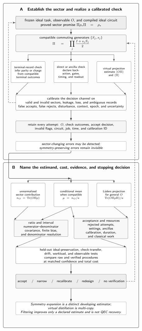
Symmetry-verification audit from an ideal-sector promise through calibrated checks, projected estimands, covariance, acceptance, and validation — Symmetry verification begins with a proved ideal-sector promise and a declared estimand. Terminal records, direct checks, and virtual projector correlations have different measurement and backaction costs, but all require calibration of false decisions, leakage, loss, drift, and transfer. Sector-changing errors may be detected; symmetry-preserving errors remain invisible. The reported conditional or projected estimate must retain numerator–denominator covariance, acceptance, rejected attempts, and held-out validation. Filtering is not QEC recovery.

Freeze the Ideal-Sector Promise and Estimand

Declare the target state, circuit, symmetry, and sector

A usable record begins with more than the name of a conservation law. State the ideal input family, ideal unitary or channel, compiled ideal circuit, observable $O$ , symmetry generators, target eigenvalues, parameter and layout domain, and the point at which the sector is checked. If the input is mixed, specify whether every component or only its total support lies in the sector. If a classical objective has a symmetry, distinguish symmetry of that objective from support of the quantum state used to estimate it. Shaydulin and Galda (2021) and Kakkar et al. (2022) analyze symmetry filtering for particular QAOA constructions and noise regimes; those application results do not establish a sector promise for an arbitrary mixer, initialization, graph, or compiled implementation.

Prove preservation across the implemented ideal circuit

Commutation of a model Hamiltonian with $S$ is only the first step. For an ideal gate sequence $U_L\cdots U_1$ , either prove $[U_k,S]=0$ for every operation or prove preservation by the complete product, including basis changes, mappings, controls, resets, and feedforward. Parameterized gates must preserve the sector throughout the declared parameter domain. Compilation can break a high-level symmetry through approximation, qubit routing, tapering conventions, or an omitted phase convention even when the intended algorithm does not. A mid-circuit measurement may create branches with different sector labels. Test the compiled ideal circuit on representative and boundary inputs before attributing departures in hardware data to noise.

Fix observable compatibility before acquisition

For a terminal record to provide both $O$ and a sector decision, the relevant observables must be jointly measurable in that acquisition context. The common shortcut $\operatorname{Tr}(O\Pi\rho)$ is guaranteed to be real and to have the required direct interpretation when $[O,\Pi]=0$ . Otherwise the Lüders numerator is $\operatorname{Tr}(O\Pi\rho\Pi)$ , and a one-sided product is not the projected expectation. A nondemolition check followed by $O$ may implement that sequential instrument, but its backaction and extra noise belong to the protocol. Mitarai and Fujii (2019) give conditions under which indirect unitary measurements can be replaced by sequences of direct measurements; their methodology supports protocol-specific simplification, not a general license to treat incompatible observables as one classical record.

Predeclare the estimand and stop rule

Before collecting science data, choose among the raw expectation, acceptance, unnormalized sector contribution, retained-record conditional mean, Lüders-projected mean, or a developing expansion estimator. Freeze whether mitigation is tuned on separate records, what denominator resolution is required, the absolute or relative precision target, and the maximum attempts, circuit executions, calibration shots, and wall time. Define a no-report event when no shot is accepted, the acceptance interval includes an unusable region, or a signed denominator is too poorly resolved. Predeclaration prevents a high-acceptance subset, favorable generator, or estimator order from being selected after inspecting the final holdout.

Build Sector Projectors from Commuting Symmetries

Binary symmetry projectors

For a Hermitian involution $S^2=I$ , the eigenvalues are $\pm1$ . The projector onto target eigenvalue $s\in\{-1,+1\}$ is

\Pi_s=\frac{I+sS}{2}, \qquad \Pi_s^2=\Pi_s=\Pi_s^\dagger.

Idempotence follows from $S^2=I$ , and Hermiticity follows from $S=S^\dagger$ . The complementary sector has $\Pi_{-s}=I-\Pi_s$ . Freeze the support promise separately as

\Pi_s\rho_\star\Pi_s=\rho_\star.

Parity, particle-number parity, spin parity, and global bit-flip sectors often enter through such involutions, but the abstract formula does not select the correct sign. The state preparation and ideal dynamics determine $s$ ; choosing the more favorable sign after seeing data is selection.

Spectral projectors beyond binary eigenvalues

If a conserved observable $Q$ has spectral resolution $Q=\sum_q q\Pi_q$ , verification can target one eigenspace $\Pi_{q_0}$ or a predeclared union of eigenspaces. Degeneracy is allowed: the projector preserves the entire eigenspace rather than selecting an arbitrary basis vector within it. A coarse accepted set $\Delta$ uses $\Pi_\Delta=\sum_{q\in\Delta}\Pi_q$ . The set must be fixed by the ideal task, not by which outcomes survive hardware noise. Continuous spectra, approximate conserved quantities, and tolerance windows require a resolution model and are outside the automatic discrete-sector license; a numerical window changes both false decisions and the target.

Products and group averages for commuting checks

For $m$ commuting binary generators $S_j$ and target signs $s_j$ , the joint projector is

\begin{aligned} \Pi_{\boldsymbol s} &:=\prod_{j=1}^{m}\frac{I+s_jS_j}{2}\\ &=\frac{1}{2^m} \sum_{A\subseteq\{1,\ldots,m\}} \left(\prod_{j\in A}s_j\right) \left(\prod_{j\in A}S_j\right). \end{aligned}

For a finite Abelian group with a declared one-dimensional character $\chi$ , the same idea becomes

\Pi_\chi := \frac{1}{|G|} \sum_{g\in G}\chi(g)^*U_g.

Cai (2021, symmetry expansion) uses this group-projector viewpoint to organize exact verification and weighted extensions. The compact notation does not remove measurement cost: deterministic virtual evaluation may require many group correlators, although compatible grouping or randomized group-element sampling can trade settings against variance.

Noncommuting constraints require another design

If orthogonal projectors $P$ and $Q$ do not commute, $PQ$ is generally neither Hermitian nor idempotent. A legitimate common subspace needs its own orthogonal projector, found from the shared eigenspace rather than assumed to equal an ordered product. Alternatively, sequential measurements define an instrument such as first $P$ , then $Q$ ; reversing the order can change acceptance and the postmeasurement state. Report that order, its backaction, and its calibration. Non-Abelian symmetry sectors may be constructed with representation-theoretic irrep projectors, but that broader theory belongs to the symmetry owners. The default response to incompatible checks is redesign or a narrower claim, not multiplication.

Realize and Calibrate the Symmetry Check

Infer checks from terminal records

When the final measurement basis already reveals a symmetry label, compute it from every raw terminal record. A particle-number or parity filter on bitstrings can add no coherent gates, but it still consumes all attempted shots and depends on readout, leakage classification, and the chosen mapping. Retain the full record before filtering so alternative diagnostics and false-decision calibration remain possible. A classical parity rule is exact only on the declared report alphabet; a leaked level mapped to a computational bit can be falsely accepted. “No extra circuit” therefore means only that the check is derived from existing terminal data, not that its statistical or calibration cost vanishes.

Add ancilla or nondemolition checks

An ancilla-assisted check may coherently couple the data to an eigenvalue register and measure the ancilla before the final observable. In an ideal nondemolition realization, acceptance prepares $\Pi\rho\Pi/a$ without resolving states inside the sector. Real circuits add controlled operations, ancilla preparation and readout, idle time, and possible propagation of ancilla faults into data. A check performed early detects only errors accumulated before it; errors afterward can pass. Repeated checks change depth and selection history. Calibrate the complete instrument in the same layout and schedule as science, including backaction on accepted states, rather than quoting only ancilla assignment fidelity.

Use virtual projection from measured correlations

For binary $S$ , target sign $s$ , and $[O,S]=0$ , substitute $\Pi_s=(I+sS)/2$ into the conditional ratio:

\mu_s := \frac{\langle O\rangle+s\langle OS\rangle} {1+s\langle S\rangle}.

This post-processing estimator is often called virtual symmetry verification: no selective sector measurement need occur, but the observable, symmetry, and product correlations must be measured with a declared grouping and shot allocation. Bonet-Monroig et al. (2018) derive the identity, while Huggins et al. (2021) compare direct postselection with correlation-based evaluation in a chemistry measurement setting. “Virtual” here does not mean virtual distillation and does not remove the denominator or its variance.

Calibrate false accepts and false rejects

Let $T=1$ denote true valid-sector membership and $A=1$ the observed accept decision. Define the prevalence $\pi=\Pr(T=1)$ , true-accept probability $\alpha=\Pr(A=1\mid T=1)$ , and false-accept probability $\beta=\Pr(A=1\mid T=0)$ . If decision rates are constant within each latent sector, then

\mathbb E[O\mid A=1] = \frac{\alpha\pi\mu_{\rm in} +\beta(1-\pi)\mu_{\rm out}} {\alpha\pi+\beta(1-\pi)}.

False accepts contaminate the numerator. Uniform false rejection, $1-\alpha$ , lowers acceptance; it also biases when acceptance varies with $O$ , a state within the valid sector, circuit context, or time. Calibrate the full decision channel on resolved valid, invalid, leakage, loss, and ambiguous fixtures with uncertainty.

Retain invalid, leakage, loss, and failure records

Every attempted execution belongs in the acquisition ledger, including shots for which the observable is absent, the check is ambiguous, a classifier reports leakage, a job fails, or a timeout occurs. Collapsing these events into rejection can conceal different physical and statistical processes. Dropping them before normalization changes acceptance and can make the procedure look cheaper or cleaner than it is. Leakage and Crosstalk owns enlarged-sector physics; this page owns the decision rule and accepted-answer accounting. Store raw outcome, decision category, circuit and parameter identifiers, layout, job, timestamp, and calibration version so loss, drift, and transfer can be audited.

Separate Conditional, Projected, and Unnormalized Targets

Acceptance and the unnormalized sector contribution

For a noisy state $\rho$ , define the sector weight and, for a compatible observable, its one-sided sector moment by

a=\operatorname{Tr}(\Pi\rho), \qquad n_O=\operatorname{Tr}(O\Pi\rho) \quad\text{when }[O,\Pi]=0.

The operator $\widetilde\rho_\Pi=\Pi\rho\Pi$ and the moment $n_O$ are unnormalized: $\operatorname{Tr}(\widetilde\rho_\Pi)=a$ . Thus $n_O$ combines how much state weight survives with the observable inside that weight. It is useful as the numerator of a ratio and may remain reportable when the ratio is unstable, but it is not a conditional expectation. Acceptance itself is a resource and diagnostic quantity, not fidelity; an accepted state can contain substantial symmetry-preserving error.

Conditional expectations for compatible observables

If $O$ and $\Pi$ commute and the decision realizes the intended sector without misclassification, the normalized conditional target is

\mu_{\rm cond}=\frac{n_O}{a}.

For same-record postselection, this is the population mean of $O$ among accepted records. It differs from the raw $\operatorname{Tr}(O\rho)$ whenever rejected and accepted sectors have different means. It equals the intended ideal target $\operatorname{Tr}(O\rho_\star)$ only if the ideal-support promise is correct and the remaining within-sector error does not bias that observable beyond the stated tolerance. A favorable conditional value can coexist with declining acceptance, so both quantities and the attempted-shot count must be shown.

Lüders projection for general observables

The normalized state associated with an ideal selective projection is

\rho_{\rm L} := \frac{\Pi\rho\Pi}{\operatorname{Tr}(\Pi\rho)},

and its observable mean is

\mu_{\rm L} := \frac{\operatorname{Tr}(O\Pi\rho\Pi)} {\operatorname{Tr}(\Pi\rho)}.

When $[O,\Pi]=0$ , cyclicity and idempotence give $\mu_{\rm L}=\mu_{\rm cond}$ . Without compatibility, $\operatorname{Tr}(O\Pi\rho)/a$ is not the Lüders mean and can even be complex. Implementing $\mu_{\rm L}$ requires an actual sequential instrument or an independently justified correlation protocol. Degenerate Measurements and Lüders Rule owns the general state-update theory; here it fixes the verification estimand.

Symmetry expansion is a distinct estimator family

Exact group projection uses uniform character weights. Symmetry expansion replaces that projector by a selected linear combination $\Gamma$ and evaluates, in a compatible realization,

\mu_\Gamma := \frac{\operatorname{Tr}(O\Gamma\rho)} {\operatorname{Tr}(\Gamma\rho)}.

Cai (2021, symmetry expansion) develops weights that trade estimation bias against sampling cost. Unless $\Gamma$ is the exact positive projector appropriate to the task, the quotient need not describe a postselected physical state; cancellation can be the intended mechanism. Tsubouchi et al. (2023) extend related ideas to virtual quantum error detection, and Yoshioka et al. (2022) develop generalized quantum subspace expansion with broader state powers and error-boosted subspaces. These are developing, protocol-specific estimator families, not synonyms for ordinary single-copy sector verification.

Reported object	Formula	Ideal-support license	Measurement record	Covariance need	Dominant failure	Claim boundary
Raw expectation	$\operatorname{Tr}(O\rho)$	Raw target declared	All observable records	Ordinary estimator covariance	Hardware bias	No sector filtering
Acceptance probability	$a=\operatorname{Tr}(\Pi\rho)$	Declared sector and check	Every accept and reject	Binomial or full decision covariance	Misclassification or loss	Not fidelity
Unnormalized sector contribution	$n_O=\operatorname{Tr}(O\Pi\rho)$	$[O,\Pi]=0$	Accepted-weighted observable	With $a$ if normalized later	Conflates weight and mean	Numerator only
Direct conditional mean	$\mathbb E[O\mid A=1]$	Ideal support and calibrated decision	Same-record $O,A$ pairs	Same-record ratio covariance	Selection and false accepts	Conditional population
Lüders-projected mean	$\operatorname{Tr}(O\Pi\rho\Pi)/a$	Selective projection instrument	Project then measure $O$	Numerator–acceptance covariance	Backaction or instrument error	Projected state mean
Virtual projector expansion	$(\langle O\rangle+s\langle OS\rangle)/(1+s\langle S\rangle)$	Binary symmetry and compatibility	Correlation settings	Full shared or allocated covariance	Small denominator	Exact projector quotient
Symmetry expansion or reweighting	$\operatorname{Tr}(O\Gamma\rho)/\operatorname{Tr}(\Gamma\rho)$	Declared weighted estimator	Weighted group correlations	Signed numerator–denominator covariance	Bias and sign cancellation	Not necessarily a state

Proposed claim	Required license	Primitive record	Diagnostic	Falsifier	Response	Residual claim
Ideal-sector support	$\Pi\rho_\star\Pi=\rho_\star$ on the declared family	Ideal states or certified reference	Out-of-sector mass	Nonzero ideal leakage	Redesign promise	No filtering claim
Implemented ideal preservation	Compiled ideal circuit preserves the sector	Gate-level ideal simulations	Sector by layer and parameter	Compiled sector drift	Repair compilation	Model-level symmetry only
Observable and check compatibility	Joint record or explicit sequential instrument	Observable and check settings	Commutator and backaction test	Incompatible shortcut	Use Lüders protocol	Separate observables only
Check calibration	Decision channel resolved in context	Valid, invalid, leakage, and loss fixtures	False decisions with intervals	Unidentified class or drift	Recalibrate or redesign	Mathematical check only
Complete outcome accounting	Every attempt and decision retained	Raw records, failures, timestamps	Count reconciliation	Dropped invalid or failed records	Restore ledger	Accepted-subset description
Stationarity and workload transfer	Calibration covers science context and epoch	Held-out circuits, layouts, and times	Transfer residuals	Context or time failure	Narrow or recalibrate	In-domain result only
Denominator resolution	Acceptance or signed denominator exceeds stop threshold	Numerator–denominator pairs	Interval and zero-crossing risk	Unresolved denominator	No report	Unnormalized moment only

Propagate Ratio Uncertainty and Acceptance Cost

Propagate the full ratio covariance

Let $\widehat\mu=\widehat n/\widehat a$ , where $\widehat n$ and $\widehat a$ may be constructed from shared or separately allocated records. Linearizing around population values gives

\operatorname{Var}(\widehat\mu) \approx \frac{ \operatorname{Var}(\widehat n) +\mu^2\operatorname{Var}(\widehat a) -2\mu\operatorname{Cov}(\widehat n,\widehat a) }{a^2}.

The covariance term can increase or decrease uncertainty; setting it to zero is an experimental-design claim, not a harmless simplification. The second-order expansion also retains the leading quotient bias

\mathbb E[\widehat\mu]-\mu \approx \frac{ \mu\operatorname{Var}(\widehat a) -\operatorname{Cov}(\widehat n,\widehat a) }{a^2}.

Cai (2021, symmetry expansion) gives the quotient-variance accounting for symmetry-based estimators, while Cai et al. (2023) place ratio covariance and sampling overhead in the wider mitigation framework. Preserve shot identifiers or grouping metadata so covariance can be reconstructed.

Control finite-sample and small-denominator risk

For direct same-record filtering, write $A_i\in\{0,1\}$ for acceptance and $K=\sum_iA_i$ . Conditional on $K>0$ , the retained average $K^{-1}\sum_iA_iO_i$ is unbiased for the accepted population when records are independent and the decision rule is fixed. Its numerator and denominator covariance makes the leading quotient-bias terms cancel. This is not the same as a plug-in ratio assembled from separately estimated expectations. Moreover,

\Pr(K=0)=(1-a)^N,

so an empty accepted sample is a real outcome, not a value of zero. More generally, a weak, signed, or calibration-corrected denominator can cross zero and produce heavy-tailed ratios for which a delta interval is misleading. Use a predeclared denominator threshold, inspect joint bootstrap or likelihood behavior, and issue no report rather than clipping or silently enlarging the run. Sagastizabal et al. (2019) observed finite-sampling pathologies in projected reconstructions, including loss of positivity, underscoring that algebraic projection does not make finite estimates physical.

Count attempts per accepted result

For direct same-record postselection, the leading variance is

\operatorname{Var}(\widehat\mu) \approx \frac{\operatorname{Var}(O\mid A=1)}{Na}.

Obtaining a fixed expected number of retained records therefore requires approximately $1/a$ attempts per retained record. Correlation-based virtual projection often has approximately a $1/a^2$ precision cost because noisy estimates of both numerator and denominator are divided by $a$ . Huggins et al. (2021) make this direct-versus-post-processing distinction, but neither coefficient is universal: the conditional variance, covariance, grouping, allocation, and baseline estimator matter. Separately report attempted circuits, accepted records, rejected and invalid records, added gates and ancillas, calibration shots, resets, wall time, and classical processing. A method that reduces bias while exhausting the frozen budget is not accepted.

Allocate measurements across projected terms

A virtual projector expands into observable–symmetry products, and different terms can have different variances, circuit depths, and compatible measurement groups. For an independent linear sum $L=\sum_k c_kX_k$ with fixed total shots, the familiar variance-only allocation scales as $N_k\propto |c_k|\sigma_k$ . A projected ratio is harder: numerator and denominator reuse some terms, grouped outcomes create covariance, and an allocation optimized for the numerator alone can leave $a$ unresolved. Pilot data may set an allocation only before the final holdout and within a frozen rule. Record each term, coefficient, grouping, shots, empirical covariance, and circuit cost. Random group-element sampling is a valid alternative when its sampling law and weights are explicit; it trades deterministic settings for another source of variance rather than erasing the expansion.

Combine Multiple Symmetries without Double Counting

Expand the joint projector before simplifying

For two commuting binary checks, write the complete projector before designing measurements:

\Pi_{s_1,s_2} = \frac{1}{4} \left(I+s_1S_1+s_2S_2+s_1s_2S_1S_2\right).

For compatible $O$ , both $\langle\Pi_{s_1,s_2}\rangle$ and $\langle O\Pi_{s_1,s_2}\rangle$ contain the cross term. Omitting it does not implement the intersection of sectors. Bonet-Monroig et al. (2018) emphasize that commuting symmetries can be combined, whereas sequential noncommuting checks are a different problem. After the exact expansion is fixed, algebraic relations and measurement grouping may reduce work. Simplification must preserve the operator identity, target signs, and covariance of the retained terms.

Treat redundant checks as correlated evidence

If one generator is the product of others on the represented Hilbert space, its eigenvalue is constrained and it is not an independent sector restriction. Keeping it can still diagnose a faulty measurement channel, but the resulting decisions are correlated evidence rather than additional independent acceptance. Even independent algebraic generators can have correlated hardware outcomes because one physical fault flips several checks or because their readout shares a classifier. For accept indicators $A_1,A_2$ ,

\Pr(A_1=A_2=1) = \mathbb E[A_1A_2] \ne \mathbb E[A_1]\mathbb E[A_2]

unless factorization is validated. Report generator relations, joint counts, and the acceptance covariance instead of multiplying marginal pass rates.

Record acceptance collapse and selection order

The accepted fraction for a joint projector is $a_{12}=\operatorname{Tr}(\Pi_{s_1,s_2}\rho)$ , not a product inferred from separate experiments. Requesting $M$ doubly accepted records costs about $M/a_{12}$ attempts under stationary independent trials. Adding a correct constraint cannot enlarge the exact intersection, but an imperfect physical check can produce nonmonotone observed rates through false decisions and disturbance. If checks are performed sequentially, record their order and the conditional pass rate at each stage; an early rejection saves later work but changes which records reach later calibrations. Choose the generator set, order, and stopping threshold before final data. A dramatic acceptance collapse can make the joint estimator unusable even when each marginal check looks benign.

Audit Detectable, Invisible, and Misclassified Errors

Sector-changing errors are potentially visible

An error component is detectable by a sector test when it maps supported ideal states outside the accepted subspace. For a binary check, anticommutation is a convenient sufficient test for a Pauli component, but the physical detection probability also depends on when the error occurs, whether later operations return it to the sector, and whether the check is read correctly. The rejected fraction therefore cannot be assigned to a unique error rate. McArdle, Yuan, and Benjamin (2019) reported 60–80% detection for depolarizing errors in their specific digital-simulation study; the percentage is evidence for that model and circuit, not a hardware-independent sensitivity. Calibrate injected or otherwise resolved sector-changing fixtures to measure the realized decision channel.

Symmetry-preserving errors remain invisible

A coherent rotation within the target sector, dephasing generated by the checked symmetry, and any fault commuting with every checked generator can pass with probability one under an ideal check. Such faults may strongly bias $O$ . Sagastizabal et al. (2019) demonstrated symmetry verification for a two-qubit hydrogen VQE and found substantial improvement in that experiment, while also distinguishing detectable relaxation-related effects from dephasing and optimizer limitations. This is the correct scope: verification can suppress selected error components in a measured workload. It cannot certify that the accepted density operator is close to the target, and an energy or fidelity improvement measured on one circuit does not establish improvement for every observable.

Promise breaking creates selection bias

If the ideal task has genuine support outside $\Pi$ , conditioning removes valid signal. Examples include a state intentionally superposing charge sectors, a symmetry-breaking perturbation retained in the model, a time-dependent control that does not commute with the generator, and an approximation whose truncation breaks the conservation law. The filtered answer can then look smoother because it estimates a different population. Detect promise breaking with ideal simulations, analytical commutators, boundary parameters, and reference experiments before hardware filtering. If the symmetry is only approximate, specify a tolerance model and report the changed estimand; do not hide approximation error inside a false-accept rate. The proper decision may be to narrow the parameter domain or not verify.

An imperfect check can worsen the answer

With constant sector-level decision rates, accepted contamination is

c_{\rm out} := \frac{\beta(1-\pi)} {\alpha\pi+\beta(1-\pi)}.

The accepted mean differs from the true in-sector mean by $c_{\rm out}(\mu_{\rm out}-\mu_{\rm in})$ . A small false-accept probability can therefore matter when out-of-sector prevalence or mean contrast is large. False rejection raises cost and becomes bias when it depends on the observable or state. Ancilla faults can additionally disturb accepted data, which this label-confusion model does not describe. Compare the calibrated, filtered estimator with the matched raw baseline using independent reference truth and total resources. If the check adds more bias or variance than it removes, recalibrate, redesign, or abstain.

Compose Symmetry Filtering with Other Mitigation

Correct the joint measurement record before filtering

When readout can change a sector label, measurement mitigation acts on the joint observable-and-check alphabet before a hard decision. A response model for only the accepted histogram cannot reconstruct valid records that were falsely rejected and discarded. Retain counts $q_{\widetilde o,\widetilde a}$ , calibrate the licensed response from latent $(o,a)$ to reported $(\widetilde o,\widetilde a)$ , propagate its uncertainty, and only then form projected moments. Bravyi et al. (2021) show how multiqubit measurement correction depends on explicit response assumptions; here those assumptions also control selection. If calibration and science records or multiple projected terms share response parameters, carry the induced covariance. Negative components from an inverse are diagnostics or quasiprobability weights, not probabilities to clip before the ratio.

Choose the ZNE numerator–denominator order

Let $\lambda$ label the effective noise gain. One composite protocol forms

R(\lambda)=\frac{n(\lambda)}{a(\lambda)}

at every gain and extrapolates $R(\lambda)$ . Another extrapolates the paired numerator and denominator and then forms $R(0)=n(0)/a(0)$ . Nonlinearity, finite fit order, covariance, and small denominators make these different estimators. Cai (2021, multi-exponential extrapolation) studies combinations of symmetry verification, extrapolation, and quasiprobability techniques under specified Pauli-noise models and leaves more general noise behavior open. Freeze the order, gain definition, shared records, fit family, and acceptance $a(\lambda)$ before validation. Never extrapolate a numerator while silently using a denominator from another gain.

Combine PEC weights and filters without hiding signs

Probabilistic error cancellation produces signed circuit weights. If $w_i$ is the PEC weight and $A_i$ a sector decision, a natural estimator-level composition retains signs in both parts,

\widehat\mu_{\rm PEC+SV} := \frac{\sum_i w_iA_iO_i} {\sum_i w_iA_i}.

Renormalizing an accepted subset separately inside each sampled recovery circuit generally changes the quasiprobability identity because acceptance can correlate with circuit choice, sign, and magnitude. The signed denominator may be small even when the unweighted acceptance is high. Probabilistic Error Cancellation owns implementable-basis inversion and signed-sampling theory; this page owns the added sector decision, ratio, and acceptance record. Cai (2021, symmetry expansion) recommends post-processing numerator and denominator when composing such methods. Validate the entire stack, and charge both overheads.

Protect adaptive loops from selection effects

In VQE, QAOA, or another hybrid loop, a filtered objective changes which parameters the optimizer visits. If generator choice, decision thresholds, measurement allocation, or mitigation hyperparameters are tuned on those same records, the final reported minimum inherits adaptive selection bias. Endo et al. (2021) review hybrid quantum–classical mitigation and emphasize that practical conclusions depend on the complete algorithmic workflow. Separate records for adaptation, mitigation tuning, validation, and final reporting; freeze the chosen stack before the final holdout. Report both raw and filtered trajectories at matched resources, not only the lowest filtered point. A method that improves an objective during tuning but fails on fresh circuits supports at most a narrow diagnostic claim.

Validate on Held-Out Circuits and Decide

Calibrate the full decision channel

A single “assignment fidelity” cannot characterize a selector. At minimum, estimate true acceptance, false acceptance, and the corresponding rejections with intervals on valid and invalid fixtures. Add resolved leakage, loss, and ambiguous classes when they occur. Then test whether the decision probability varies with the observable, state within a sector, circuit depth, layout, neighboring activity, parameter, or time. Such dependence invalidates the constant-rate mixture formula unless modeled explicitly. For a direct check, also characterize accepted-state backaction; for a virtual check, characterize every measured correlation and grouping. Keep calibration records independent of the final science holdout and version the decision rule so recalibration does not retroactively change which records were accepted.

Test held-out transfer, time, and circuit context

Validation has seven layers: verify projector Hermiticity, idempotence, eigenvalues, commutation, and normalization; prove input support and compiled ideal preservation; calibrate the realized check; reconcile every science attempt; propagate ratio covariance and apply the no-report rule; test fresh circuits, parameters, layouts, observables, epochs, and drift; then compare raw and filtered estimates at matched output quality, confidence, and total resources. Reference truth may come from exact small instances, trusted simulators within their license, conservation-independent observables, or cross-platform checks. A benchmark used to choose generators or thresholds is tuning data, not validation. Transfer failure narrows the claim even when the original benchmark remains favorable.

Report the complete symmetry-verification record

The result must be reconstructible from primitive records. Name the exact sector, generator signs, mapping, compiled circuit, check implementation, outcome alphabet, decision channel, estimator order, covariance method, denominator rule, validation split, and all resources. Report raw and mitigated point estimates with intervals, acceptance with uncertainty, attempted and retained counts, failures, and any abstentions. Reporting Standards owns durable provenance; the ledger below identifies the symmetry-specific fields that provenance must retain.

Ledger item	Primitive record	Transformation	Uncertainty	Diagnostic	Resource unit	Claim boundary
Sector promise	Ideal state family and target eigenvalues	Support test	Reference uncertainty	Out-of-sector ideal mass	Reference evaluations	Declared domain only
Projector and generators	Matrices, Pauli words, signs, relations	Product or group average	Algebraic tolerance	Hermiticity and idempotence	Terms and settings	Commuting construction only
Circuit and compiler	Logical and compiled operations	Preservation audit	Simulation or bound	Layerwise sector drift	Gates, depth, layouts	Implemented ideal circuit
Check realization	Terminal rule or ancilla instrument	Decision extraction	Backaction and readout error	Context comparison	Added gates, ancillas, time	Realized check only
Science acquisition	All outcomes, decisions, IDs, and times	Raw and filtered summaries	Shot covariance	Count reconciliation	Attempts and accepted shots	Frozen acquisition domain
Check calibration	Valid, invalid, leakage, and loss fixtures	Decision-channel fit	Parameter covariance	False decisions and drift	Calibration circuits	Calibrated classes only
Estimator and covariance	Numerator–denominator records and weights	Conditional, Lüders, or expanded ratio	Full joint interval	Denominator and sign risk	Terms and classical work	Named estimand only
Held-out validation and failures	Fresh contexts and reference targets	Matched raw–filtered comparison	Coverage and transfer intervals	Residual, drift, abstention	Validation circuits	Passed holdout domain
Total resources	Executions, resets, failures, compute, and time	Budget aggregation	Run-to-run variation	Cost versus frozen cap	Device time and compute	Matched-resource claim

Accept, narrow, recalibrate, redesign, or do not verify

Accept only when the ideal support, compiled preservation, compatibility, check calibration, complete accounting, denominator resolution, covariance, stationarity, and held-out transfer jointly license the prespecified claim. Narrow when evidence covers only one sector, observable family, circuit depth, layout, epoch, noise family, or estimator. Recalibrate when resolvable false decisions, response drift, or leakage and loss classification failed without exposing the final holdout. Redesign when another generator set, check realization, grouping, acquisition schedule, or estimand could restore a valid test. Do not verify when the promise is false, checks are incompatible or unidentifiable, symmetry-preserving bias dominates, acceptance is unresolved or too small, validation fails, or total cost exceeds the frozen budget. Abstention is a scientific result, not a missing data point.

Three Reproducible Finite Audits

Audit 1 — binary projection and ratio covariance

Order the joint probabilities as $(S,O)=(+,+),(+,-),(-,+),(-,-)$ and take $(0.54,0.18,0.08,0.20)$ with target sector $s=+1$ and $N=20000$ science attempts. Direct summation gives

\begin{aligned} \langle O\rangle&=0.24, &\langle S\rangle&=0.44, &\langle OS\rangle&=0.48,\\ a&=0.72, &n_O&=0.36, &\mu&=0.50. \end{aligned}

For $X=O\mathbf{1}_A$ and $Y=\mathbf{1}_A$ , one obtains $\operatorname{Var}(X)=0.5904$ , $\operatorname{Var}(Y)=0.2016$ , and $\operatorname{Cov}(X,Y)=0.1008$ . The complete delta variance is $0.00005208333333333332$ , with standard error $0.007216878364870321$ . Omitting the positive covariance would overstate this variance. The raw mean $0.24$ , unnormalized contribution $0.36$ , and conditional mean $0.50$ are not competing estimates of one unspecified object; they answer three different questions.

Audit 2 — an imperfect symmetry classifier

Set valid-sector prevalence $\pi=0.75$ , true-accept probability $\alpha=0.92$ , false-accept probability $\beta=0.10$ , valid-sector mean $0.40$ , invalid-sector mean $-0.60$ , and request $5000$ accepted records. The observed acceptance is $0.715$ and the accepted numerator is $0.261$ , giving mean $0.365034965034965$ . Its bias relative to the valid-sector mean is $-0.034965034965035$ , beyond the absolute tolerance $0.02$ . Invalid records make up $0.03496503496503496$ of the accepted sample. Per attempt, false rejection has probability $0.06$ and false acceptance probability $0.025$ ; the expected attempt count is $6993.006993006992$ . The decision is recalibrate or do not verify.

This calculation assumes decision rates constant within each latent sector. If acceptance depends on $O$ , state, time, or context, two numbers $(\alpha,\beta)$ do not identify the selection bias. Stratified or otherwise richer calibration is required.

Audit 3 — correlated commuting checks

Order the outcomes and their probabilities as the following matched sequences:

\begin{aligned} \bigl((S_1,S_2,O)_j\bigr)_{j=1}^{8} ={}&\bigl((+,+,+),(+,+,-),(+,-,+),(+,-,-),\\ &\qquad (-,+,+),(-,+,-),(-,-,+),(-,-,-)\bigr),\\[2pt] (p_j)_{j=1}^{8} ={}&\bigl(0.42,0.14,0.08,0.06,\\ &\qquad 0.10,0.05,0.06,0.09\bigr). \end{aligned}

With $N=25000$ , the raw observable mean is $0.32$ . The marginal acceptances are $a_1=0.70$ and $a_2=0.71$ , but joint acceptance is $0.56$ and $\operatorname{Cov}(A_1,A_2)=0.063$ ; the wrong independence product is $0.497$ .

The measured moments are $\langle S_1\rangle=0.40$ , $\langle S_2\rangle=0.42$ , $\langle S_1S_2\rangle=0.42$ , $\langle OS_1\rangle=0.28$ , $\langle OS_2\rangle=0.34$ , and $\langle OS_1S_2\rangle=0.18$ . The expanded projector gives numerator $0.28$ and doubly conditioned mean $0.50$ . Requesting $6000$ accepted records requires $10714.285714285714$ expected attempts from the joint rate, not the independence-based $12072.434607645875$ . The same-record ratio variance is $0.000053571428571428575$ and its standard error is $0.007319250547113999$ . Compatible commuting checks may still have correlated decisions; measure the joint acceptance instead of multiplying marginals.

The following dependency-free audit reconstructs every stated result from the primitive probabilities, uses absolute tolerance $10^{-12}$ , and prints one line only.

const tolerance = 1e-12;

function close(actual, expected, label) {
  if (!Number.isFinite(actual) || Math.abs(actual - expected) > tolerance) {
    throw new Error(`${label}: ${actual} versus ${expected}`);
  }
}

function checkProbabilities(probabilities, label) {
  probabilities.forEach((value, place) => {
    if (value < 0 || value > 1) throw new Error(`${label}[${place}]`);
  });
  close(probabilities.reduce((total, value) => total + value, 0), 1, `${label} sum`);
}

function expectation(probabilities, states, value) {
  return probabilities.reduce(
    (total, probability, place) => total + probability * value(states[place]),
    0,
  );
}

const probabilitiesOne = [0.54, 0.18, 0.08, 0.20];
const statesOne = [[1, 1], [1, -1], [-1, 1], [-1, -1]];
const scienceAttemptsOne = 20000;
checkProbabilities(probabilitiesOne, 'audit one probabilities');

const rawObservableOne = expectation(probabilitiesOne, statesOne, ([, observable]) => observable);
const symmetryMeanOne = expectation(probabilitiesOne, statesOne, ([symmetry]) => symmetry);
const observableSymmetryOne = expectation(
  probabilitiesOne,
  statesOne,
  ([symmetry, observable]) => symmetry * observable,
);
const acceptanceOne = expectation(probabilitiesOne, statesOne, ([symmetry]) => symmetry === 1 ? 1 : 0);
const numeratorOne = expectation(
  probabilitiesOne,
  statesOne,
  ([symmetry, observable]) => symmetry === 1 ? observable : 0,
);
const conditionalOne = numeratorOne / acceptanceOne;
const varianceNumeratorOne = acceptanceOne - numeratorOne ** 2;
const varianceAcceptanceOne = acceptanceOne * (1 - acceptanceOne);
const covarianceOne = numeratorOne - numeratorOne * acceptanceOne;
const ratioVarianceOne = (
  varianceNumeratorOne
  + conditionalOne ** 2 * varianceAcceptanceOne
  - 2 * conditionalOne * covarianceOne
) / (scienceAttemptsOne * acceptanceOne ** 2);
const ratioStandardErrorOne = Math.sqrt(ratioVarianceOne);

close(rawObservableOne, 0.24, 'audit one raw observable');
close(symmetryMeanOne, 0.44, 'audit one symmetry mean');
close(observableSymmetryOne, 0.48, 'audit one observable symmetry');
close(acceptanceOne, 0.72, 'audit one acceptance');
close(numeratorOne, 0.36, 'audit one numerator');
close(conditionalOne, 0.5, 'audit one conditional mean');
close(varianceNumeratorOne, 0.5904, 'audit one numerator variance');
close(varianceAcceptanceOne, 0.2016, 'audit one acceptance variance');
close(covarianceOne, 0.1008, 'audit one covariance');
close(ratioVarianceOne, 0.00005208333333333332, 'audit one ratio variance');
close(ratioStandardErrorOne, 0.007216878364870321, 'audit one ratio standard error');

const prevalenceTwo = 0.75;
const trueAcceptTwo = 0.92;
const falseAcceptTwo = 0.10;
const validMeanTwo = 0.40;
const invalidMeanTwo = -0.60;
const requestedAcceptedTwo = 5000;
const biasToleranceTwo = 0.02;

const acceptanceTwo = trueAcceptTwo * prevalenceTwo + falseAcceptTwo * (1 - prevalenceTwo);
const numeratorTwo = (
  trueAcceptTwo * prevalenceTwo * validMeanTwo
  + falseAcceptTwo * (1 - prevalenceTwo) * invalidMeanTwo
);
const observedMeanTwo = numeratorTwo / acceptanceTwo;
const biasTwo = observedMeanTwo - validMeanTwo;
const contaminationTwo = falseAcceptTwo * (1 - prevalenceTwo) / acceptanceTwo;
const falseRejectPerAttemptTwo = (1 - trueAcceptTwo) * prevalenceTwo;
const falseAcceptPerAttemptTwo = falseAcceptTwo * (1 - prevalenceTwo);
const expectedAttemptsTwo = requestedAcceptedTwo / acceptanceTwo;
const decisionTwo = Math.abs(biasTwo) > biasToleranceTwo
  ? 'recalibrate or do not verify'
  : 'accept within tolerance';

close(acceptanceTwo, 0.715, 'audit two acceptance');
close(numeratorTwo, 0.261, 'audit two numerator');
close(observedMeanTwo, 0.365034965034965, 'audit two observed mean');
close(biasTwo, -0.034965034965035, 'audit two bias');
close(contaminationTwo, 0.03496503496503496, 'audit two contamination');
close(falseRejectPerAttemptTwo, 0.06, 'audit two false rejection');
close(falseAcceptPerAttemptTwo, 0.025, 'audit two false acceptance');
close(expectedAttemptsTwo, 6993.006993006992, 'audit two attempts');
if (decisionTwo !== 'recalibrate or do not verify') throw new Error('audit two decision');

const probabilitiesThree = [0.42, 0.14, 0.08, 0.06, 0.10, 0.05, 0.06, 0.09];
const statesThree = [
  [1, 1, 1], [1, 1, -1], [1, -1, 1], [1, -1, -1],
  [-1, 1, 1], [-1, 1, -1], [-1, -1, 1], [-1, -1, -1],
];
const scienceAttemptsThree = 25000;
const requestedAcceptedThree = 6000;
checkProbabilities(probabilitiesThree, 'audit three probabilities');

const rawObservableThree = expectation(probabilitiesThree, statesThree, ([, , observable]) => observable);
const acceptanceFirstThree = expectation(probabilitiesThree, statesThree, ([first]) => first === 1 ? 1 : 0);
const acceptanceSecondThree = expectation(probabilitiesThree, statesThree, ([, second]) => second === 1 ? 1 : 0);
const jointAcceptanceThree = expectation(
  probabilitiesThree,
  statesThree,
  ([first, second]) => first === 1 && second === 1 ? 1 : 0,
);
const acceptanceCovarianceThree = jointAcceptanceThree - acceptanceFirstThree * acceptanceSecondThree;
const independenceProductThree = acceptanceFirstThree * acceptanceSecondThree;
const symmetryFirstThree = expectation(probabilitiesThree, statesThree, ([first]) => first);
const symmetrySecondThree = expectation(probabilitiesThree, statesThree, ([, second]) => second);
const symmetryProductThree = expectation(probabilitiesThree, statesThree, ([first, second]) => first * second);
const observableFirstThree = expectation(
  probabilitiesThree,
  statesThree,
  ([first, , observable]) => observable * first,
);
const observableSecondThree = expectation(
  probabilitiesThree,
  statesThree,
  ([, second, observable]) => observable * second,
);
const observableProductThree = expectation(
  probabilitiesThree,
  statesThree,
  ([first, second, observable]) => observable * first * second,
);
const projectorNumeratorThree = (
  rawObservableThree + observableFirstThree + observableSecondThree + observableProductThree
) / 4;
const projectorDenominatorThree = (
  1 + symmetryFirstThree + symmetrySecondThree + symmetryProductThree
) / 4;
const conditionalThree = projectorNumeratorThree / projectorDenominatorThree;
const expectedAttemptsThree = requestedAcceptedThree / jointAcceptanceThree;
const wrongAttemptsThree = requestedAcceptedThree / independenceProductThree;
const ratioVarianceThree = (
  1 - conditionalThree ** 2
) / (scienceAttemptsThree * jointAcceptanceThree);
const ratioStandardErrorThree = Math.sqrt(ratioVarianceThree);

close(rawObservableThree, 0.32, 'audit three raw observable');
close(acceptanceFirstThree, 0.70, 'audit three first acceptance');
close(acceptanceSecondThree, 0.71, 'audit three second acceptance');
close(jointAcceptanceThree, 0.56, 'audit three joint acceptance');
close(acceptanceCovarianceThree, 0.063, 'audit three acceptance covariance');
close(independenceProductThree, 0.497, 'audit three independence product');
close(symmetryFirstThree, 0.40, 'audit three first symmetry');
close(symmetrySecondThree, 0.42, 'audit three second symmetry');
close(symmetryProductThree, 0.42, 'audit three symmetry product');
close(observableFirstThree, 0.28, 'audit three observable first');
close(observableSecondThree, 0.34, 'audit three observable second');
close(observableProductThree, 0.18, 'audit three observable product');
close(projectorNumeratorThree, 0.28, 'audit three projector numerator');
close(projectorDenominatorThree, jointAcceptanceThree, 'audit three projector denominator');
close(conditionalThree, 0.50, 'audit three conditional mean');
close(expectedAttemptsThree, 10714.285714285714, 'audit three expected attempts');
close(wrongAttemptsThree, 12072.434607645875, 'audit three wrong attempts');
close(ratioVarianceThree, 0.000053571428571428575, 'audit three ratio variance');
close(ratioStandardErrorThree, 0.007319250547113999, 'audit three ratio standard error');

console.log('Symmetry-verification finite audits: PASS');

Canonical Handoffs and Common Claim Failures

Canonical handoffs

Noise, Channels, and Error Mitigation owns the chapter-wide intervention map, and Error Mitigation Overview owns cross-family selection and the common bias–covariance–acceptance ledger. Projectors owns general operator algebra; Why Symmetry Matters owns physical symmetry theory. Measurement Error Mitigation owns detector-response inference, Zero-Noise Extrapolation owns gain scaling and intercept fits, and Probabilistic Error Cancellation owns implementable quasiprobability inverses.

VQE and Digital Quantum Simulation own their algorithms and application interpretation. Algorithmic Benchmarking owns matched end-to-end performance comparisons. Why Quantum Error Correction Is Possible owns encoded protection and recovery. Virtual distillation is also outside this page: its multi-copy target $\rho^M/\operatorname{Tr}(\rho^M)$ suppresses nonleading eigencomponents and is not ordinary single-copy sector conditioning.

Common claim failures

Hamiltonian commutation does not prove prepared-state support or compiled-circuit preservation. Postselection changes the estimand unless ideal support and observable compatibility are established. A passed check is neither fidelity nor evidence that no error occurred: symmetry-preserving faults and paired sector flips can pass. A mathematical symmetry does not calibrate its physical check. Products of noncommuting projectors are not presumed to be projectors. A ratio without covariance, acceptance uncertainty, and a denominator stop rule has an incomplete error bar. “No extra coherent gate” does not mean zero measurement or sampling cost.

Exact direct postselection and projector identities are standard within their assumptions. Symmetry expansion, virtual error detection, and generalized subspace estimators are developing variants with protocol-specific bias and cost. A favorable hardware or numerical demonstration remains scoped to its platform, circuit, observable, and noise regime; it does not establish a restored state, transferable algorithmic gain, or scalability. Repairing one classical outcome requires a separate identifiable response or decoding model. Detection and rejection do not supply QEC recovery or fault tolerance.

Exercises

1. Prove the binary projector and virtual-ratio identity. Let $S=S^\dagger$ , $S^2=I$ , and $s=\pm1$ . Prove that $\Pi_s=(I+sS)/2$ is an orthogonal projector. Then, assuming $[O,S]=0$ , derive the virtual formula for the normalized projected expectation.

Solution

Hermiticity is immediate. Using $s^2=1$ and $S^2=I$ ,

\Pi_s^2 =\frac{I+2sS+S^2}{4} =\frac{I+sS}{2} =\Pi_s.

Compatibility gives $\operatorname{Tr}(O\Pi_s\rho\Pi_s)=\operatorname{Tr}(O\Pi_s\rho)$ . Expanding the numerator and acceptance yields $n=[\langle O\rangle+s\langle OS\rangle]/2$ and $a=[1+s\langle S\rangle]/2$ . Their ratio is $(\langle O\rangle+s\langle OS\rangle)/(1+s\langle S\rangle)$ . The identity is unusable when the denominator is unresolved.

2. Expand a two-generator sector projector. For commuting involutions $S_1,S_2$ with target signs $s_1,s_2$ , expand the joint projector. Using Audit 3 with both target signs positive, reconstruct its acceptance and compatible-observable numerator from the displayed moments.

Solution

Multiplication gives

\Pi_{s_1,s_2} =\frac14(I+s_1S_1+s_2S_2+s_1s_2S_1S_2).

For Audit 3, $a=(1+0.40+0.42+0.42)/4=0.56$ . The numerator is $(0.32+0.28+0.34+0.18)/4=0.28$ , hence the ratio is $0.50$ . The $S_1S_2$ and $OS_1S_2$ terms are required; multiplying marginal acceptances instead gives the wrong $0.497$ denominator.

3. Quantify false-accept contamination. Reproduce Audit 2 from $(\pi,\alpha,\beta)=(0.75,0.92,0.10)$ and sector means $(0.40,-0.60)$ . Compute accepted contamination, bias, false rejection per attempt, and attempts for $5000$ accepted records. State the calibration assumption.

Solution

Acceptance is $0.92(0.75)+0.10(0.25)=0.715$ . The invalid accepted weight is $0.025$ , so contamination is $0.025/0.715=0.03496503496503496$ . The numerator is $0.92(0.75)(0.40)+0.10(0.25)(-0.60)=0.261$ , giving mean $0.365034965034965$ and bias $-0.034965034965035$ . False rejection occurs with probability $(1-0.92)0.75=0.06$ , and expected attempts are $5000/0.715=6993.006993006992$ . This uses decision rates constant within each latent sector; outcome-dependent selection requires a richer model.

4. Propagate numerator–denominator covariance. Use Audit 1 to derive its ratio variance from $\operatorname{Var}(O\mathbf{1}_A)$ , $\operatorname{Var}(\mathbf{1}_A)$ , and their covariance. Explain the limiting danger as $a\to0$ and distinguish this retained-record estimator from a ratio of independent term estimates.

Solution

Substitution gives

\frac{0.5904+(0.5)^2(0.2016)-2(0.5)(0.1008)} {20000(0.72)^2} =0.00005208333333333332.

The standard error is $0.007216878364870321$ . Same-record covariance produces the conditional-mean variance and cancels the leading quotient bias when at least one record is retained. Independently measured terms generally have different covariance and a nonzero plug-in ratio bias. The $a^{-2}$ factor makes weak denominators unstable; direct accepted-shot intuition does not license reporting when $a$ is unresolved or zero accepted records occur.

5. Budget correlated acceptance decisions. In Audit 3, compute the covariance of the two accept indicators and compare the attempts needed for $6000$ jointly accepted records using the measured joint rate and a false independence assumption. Give one experimental cause of the correlation.

Solution

The joint pass rate is $0.56$ , while $a_1a_2=0.70(0.71)=0.497$ . Therefore $\operatorname{Cov}(A_1,A_2)=0.56-0.497=0.063$ . The licensed budget is $6000/0.56=10714.285714285714$ attempts. Independence would predict $6000/0.497=12072.434607645875$ , which is wrong even though both projectors commute. One physical fault can flip both checks, or both labels can share readout and leakage classification; either mechanism correlates decisions. Measure joint counts and uncertainty rather than inferring them from marginals.

6. Compare conditional and Lüders-projected estimands. Let $\Pi=|0\rangle\langle0|$ , $\rho=|+\rangle\langle+|$ , and $O=X$ . Compute $a$ , the one-sided shortcut $\operatorname{Tr}(O\Pi\rho)/a$ , and the Lüders mean. Explain why $[O,\Pi]\ne0$ invalidates the shortcut.

Solution

Here $a=\langle+|\Pi|+\rangle=1/2$ . Direct matrix multiplication gives $\operatorname{Tr}(X\Pi\rho)=1/2$ , so the one-sided quotient equals $1$ . But $\Pi\rho\Pi=|0\rangle\langle0|/2$ , and therefore

\mu_{\rm L} =\frac{\operatorname{Tr}(X\Pi\rho\Pi)}{a} =0.

The projection prepares $|0\rangle$ , whose $X$ expectation is zero. Because $[X,\Pi]\ne0$ , cyclicity and idempotence cannot convert the one-sided product into the two-sided Lüders numerator. A sequential measurement instrument or another justified protocol is required.

7. Audit composition with measurement mitigation, ZNE, and PEC. Design the estimator record for a protocol with readout correction, noise gains $\lambda$ , signed PEC weights $w$ , and a binary sector decision. Identify the required covariance and two nonequivalent ZNE orders.

Solution

At each gain and sampled PEC circuit, retain the joint raw observable-and-check outcome, sign and weight, circuit identity, and calibration version. Apply the licensed readout response to the joint alphabet before hard filtering, propagating calibration covariance. Form signed pairs $n(\lambda)=\mathbb E[wAO]$ and $a(\lambda)=\mathbb E[wA]$ with their covariance and unweighted acceptance. Either extrapolate $n$ and $a$ jointly and then divide, or form $n(\lambda)/a(\lambda)$ at each gain and extrapolate those ratios. These orders are not generally equal. A sign-cancelled denominator, gain-dependent acceptance, discarded false rejects, or failed full-stack holdout requires abstention.

8. Design a held-out symmetry-verification decision. Specify a validation split and terminal decision for a check that passes ideal algebra, calibration, and circuits through depth $40$ , but drifts on a later epoch and has unresolved acceptance at depth $60$ . Bound the scientific claim without calling the procedure error correction.

Solution

Use separate records for projector tests, compiled ideal preservation, check calibration, tuning through depth $40$ , fresh depth-and-layout holdouts, and final reporting. Freeze generator, threshold, estimator, covariance method, denominator rule, and budget before the final holdout. Accept or narrow only the earlier epoch and validated depth- $40$ domain. Recalibrate the later epoch without reusing its final holdout; at depth $60$ , issue no verification result until acceptance is resolved within budget. Report every attempt, false-decision interval, drift failure, and raw comparison. The licensed conclusion is detection and filtering in the narrow domain, not diagnosis, recovery, logical protection, or fault tolerance.

References

X. Bonet-Monroig, R. Sagastizabal, M. Singh, and T. E. O’Brien, “Low-Cost Error Mitigation by Symmetry Verification,” Physical Review A 98, 062339 (2018), doi:10.1103/PhysRevA.98.062339.
S. Bravyi, S. Sheldon, A. Kandala, D. C. McKay, and J. M. Gambetta, “Mitigating Measurement Errors in Multiqubit Experiments,” Physical Review A 103, 042605 (2021), doi:10.1103/PhysRevA.103.042605.
Z. Cai, “Quantum Error Mitigation Using Symmetry Expansion,” Quantum 5, 548 (2021), doi:10.22331/q-2021-09-21-548.
Z. Cai, “Multi-Exponential Error Extrapolation and Combining Error Mitigation Techniques for NISQ Applications,” npj Quantum Information 7, 80 (2021), doi:10.1038/s41534-021-00404-3.
Z. Cai, R. Babbush, S. C. Benjamin, S. Endo, W. J. Huggins, Y. Li, J. R. McClean, and T. E. O’Brien, “Quantum Error Mitigation,” Reviews of Modern Physics 95, 045005 (2023), doi:10.1103/RevModPhys.95.045005.
S. Endo, Z. Cai, S. C. Benjamin, and X. Yuan, “Hybrid Quantum-Classical Algorithms and Quantum Error Mitigation,” Journal of the Physical Society of Japan 90, 032001 (2021), doi:10.7566/JPSJ.90.032001.
W. J. Huggins, J. R. McClean, N. C. Rubin, Z. Jiang, N. Wiebe, K. B. Whaley, and R. Babbush, “Efficient and Noise Resilient Measurements for Quantum Chemistry on Near-Term Quantum Computers,” npj Quantum Information 7, 23 (2021), doi:10.1038/s41534-020-00341-7.
A. Kakkar, J. Larson, A. Galda, and R. Shaydulin, “Characterizing Error Mitigation by Symmetry Verification in QAOA,” 2022 IEEE International Conference on Quantum Computing and Engineering (QCE), 635–645 (IEEE, 2022), doi:10.1109/QCE53715.2022.00086.
E. Knill and R. Laflamme, “Theory of Quantum Error-Correcting Codes,” Physical Review A 55, 900–911 (1997), doi:10.1103/PhysRevA.55.900.
S. McArdle, X. Yuan, and S. Benjamin, “Error-Mitigated Digital Quantum Simulation,” Physical Review Letters 122, 180501 (2019), doi:10.1103/PhysRevLett.122.180501.
K. Mitarai and K. Fujii, “Methodology for Replacing Indirect Measurements with Direct Measurements,” Physical Review Research 1, 013006 (2019), doi:10.1103/PhysRevResearch.1.013006.
R. Sagastizabal et al., “Experimental Error Mitigation via Symmetry Verification in a Variational Quantum Eigensolver,” Physical Review A 100, 010302(R) (2019), doi:10.1103/PhysRevA.100.010302.
R. Shaydulin and A. Galda, “Error Mitigation for Deep Quantum Optimization Circuits by Leveraging Problem Symmetries,” 2021 IEEE International Conference on Quantum Computing and Engineering (QCE), 291–300 (IEEE, 2021), doi:10.1109/QCE52317.2021.00046.
K. Tsubouchi, Y. Suzuki, Y. Tokunaga, N. Yoshioka, and S. Endo, “Virtual Quantum Error Detection,” Physical Review A 108, 042426 (2023), doi:10.1103/PhysRevA.108.042426.
N. Yoshioka, H. Hakoshima, Y. Matsuzaki, Y. Tokunaga, Y. Suzuki, and S. Endo, “Generalized Quantum Subspace Expansion,” Physical Review Letters 129, 020502 (2022), doi:10.1103/PhysRevLett.129.020502.