Kraus, Choi, and Stinespring Views

A finite-dimensional completely positive map can be stored as a Kraus family, as a positive Choi operator, or as a Stinespring interaction with an auxiliary environment. These are not three competing dynamics. After conventions are fixed, they are three realizations of the same unread map, and a single Kraus-column factor makes their shared rank, nonzero spectrum, compression, and gauge freedom explicit. What changes when the environment is retained or measured is the operational question, not merely the notation.

This page develops that structural crosswalk for quantum-information work. It shows how to move between a channel and a selected trace-nonincreasing operation, how to construct minimal and padded pure-environment realizations, and how to decide which statements survive a change of Kraus or environment basis. It does not reprove the representation theorems, identify a microscopic bath from a channel, or promote an arbitrary factorization to a physical trajectory model.

Required background. Quantum Channels for QI supplies the output–input Choi convention, column vectorization, finite physicality conditions, and broader representation workflow used here. Quantum Channels and Noise supplies complete positivity, trace conditions, operations, instruments, and the Kraus, Choi, and Stinespring representation theorems used without reproof.

Helpful background. Spectral Decomposition supplies positive-operator factorization and degeneracy bookkeeping. Partial Trace supplies the subsystem reductions used to compare an unread output with a retained environment record.

Unread Maps and Their Three Realizations

Deterministic channels and selected operations

Let $\mathcal H_{\mathrm{in}}$ and $\mathcal H_{\mathrm{out}}$ be finite-dimensional. The invariant object is a completely positive linear map

$$\Phi:\mathcal B(\mathcal H_{\mathrm{in}}) \longrightarrow \mathcal B(\mathcal H_{\mathrm{out}}), \qquad \Phi(X)=\sum_{a=1}^{m}K_aXK_a^\dagger.$$

For a deterministic channel, $\sum_aK_a^\dagger K_a=I_{\mathrm{in}}$. For a selected operation, $\sum_aK_a^\dagger K_a\preceq I_{\mathrm{in}}$ and $\operatorname{Tr}\Phi(\rho)$ is the probability of the selected event. The structural equivalences below apply to either case. Trace preservation or trace nonincrease must be carried through every conversion; complete positivity alone does not determine which operational object has been represented.

An instrument $\{\mathcal I_\mu\}_\mu$ contains more information than its unread sum $\Phi=\sum_\mu\mathcal I_\mu$. Its outcome labels, probabilities, and conditional outputs remain accessible. Once those labels are discarded, different instruments can become exactly the same channel. This distinction is the reason that a basis change on a Kraus-label space may be harmless for unread propagation yet consequential when that space is measured.

The unread map is the invariant object

The three realizations store different arrays and answer different working questions, but equality is judged by the action $X\mapsto\Phi(X)$. The comparison below deliberately separates what one can recover from the stored object from what that object cannot establish by itself.

View	Stored object	Recovery of the unread map	Minimal datum	Admissible freedom	Strongest QI question	Claim not licensed
Kraus family	operators $\{K_a\}_{a=1}^m$	$\Phi(X)=\sum_aK_aXK_a^\dagger$	$r$ linearly independent operators	isometric mixing and zero padding	direct propagation and branch-aware implementation	that a label is a physical event
Choi operator	$J_\Phi\succeq0$ on output $\otimes$ input	contract $J_\Phi$ with $X^{\mathsf T}$	rank-$r$ positive support	factor phases and rotations within degenerate support	complete positivity, trace conditions, and compression	a unique factorization or bath
Stinespring realization (isometry for TP; contraction for TNI)	$V:\mathcal H_{\mathrm{in}}\to\mathcal H_{\mathrm{out}}\otimes\mathcal H_E$	$\Phi(X)=\operatorname{Tr}_E(VXV^\dagger)$	$\dim\mathcal H_E=r$ for a pure minimal realization	environment isometry and unused dimensions	complementary output and access to an environment record	microscopic bath size or synthesis cost

The common minimal number $r$ is the Choi rank. A displayed list can have $m>r$ because its members are linearly dependent or include zeros; a laboratory bath can be far larger than $r$ because a one-use reduced channel forgets microscopic structure. Equality of two realizations therefore requires an unread-map comparison first and an operational-record comparison only if an environment or outcome is actually accessible.

The narrow QI scope

The canonical formal pages own the proofs and general theorems: Kraus Representation, Choi Matrix, and Stinespring Representation. Here the purpose is narrower: turn those theorems into a convention-complete finite crosswalk, expose the shared matrix factor, and make compression and environment access auditable.

The chapter guide Noise, Channels, and Error Mitigation owns the broader discrepancy–mechanism–evidence–intervention–cost workflow. A one-use channel is not evidence of stationarity, locality, or absence of memory. Nor does its minimal dilation prescribe a gate synthesis. Those conclusions require device models, multitime experiments, or compilation data beyond the three-view equivalence.

The discussion assumes finite dimensions and a pure auxiliary state in the Stinespring construction. Mixed initial environments can be purified by enlarging the auxiliary space, but the dimension of that laboratory model need not be minimal. Infinite-dimensional continuity and domain questions, continuous measurements, and Markovian master-equation limits are outside this page’s retained scope (Breuer and Petruccione 2002; Holevo 2012).

Freeze the Realization Record

Spaces, dimensions, and output–input order

Write $d_{\mathrm{in}}=\dim\mathcal H_{\mathrm{in}}$ and $d_{\mathrm{out}}=\dim\mathcal H_{\mathrm{out}}$. A Kraus operator $K_a$ has shape $d_{\mathrm{out}}\times d_{\mathrm{in}}$. This page uses the unnormalized output–input Choi operator

$$J_\Phi = \sum_{i,j=0}^{d_{\mathrm{in}}-1} \Phi(\lvert i\rangle\!\langle j\rvert) \otimes \lvert i\rangle\!\langle j\rvert,$$

so $J_\Phi$ acts on $\mathcal H_{\mathrm{out}}\otimes\mathcal H_{\mathrm{in}}$. A trace-preserving map obeys $\operatorname{Tr}_{\mathrm{out}}J_\Phi=I_{\mathrm{in}}$ and $\operatorname{Tr}J_\Phi=d_{\mathrm{in}}$. The normalized maximally entangled convention divides this operator by $d_{\mathrm{in}}$; spectra copied from it must be rescaled before comparison.

Composite array positions are interpreted in output–input order throughout. That declaration fixes partial traces, reshaping, and the reset example below. In an exchanged data record, also state the ordered bases, matrix storage layout, and tensor-factor and index order. A positivity test cannot repair an undocumented permutation.

Vectorization, Kraus-label space, and environment basis

For an operator with entries $K_{\mu i}=\langle\mu\rvert K\lvert i\rangle$, standard column stacking and the output–input Kraus ket are related but differently ordered:

$$\operatorname{vec}_{\mathrm{col}}K =\sum_{i,\mu}K_{\mu i} \lvert i\rangle_{\mathrm{in}}\otimes\lvert\mu\rangle_{\mathrm{out}}, \qquad \lvert K\rangle\!\rangle_{\mathrm{OI}} :=S_{\mathrm{in},\mathrm{out}}\operatorname{vec}_{\mathrm{col}}K =\sum_{\mu,i}K_{\mu i} \lvert\mu\rangle_{\mathrm{out}}\otimes\lvert i\rangle_{\mathrm{in}},$$

where $S_{\mathrm{in},\mathrm{out}}$ swaps the two tensor factors. The first vector is the standard column-stacked array used in Liouville formulas; the second has exactly the output–input order of $J_\Phi$ and is used in every Choi factor below. For unequal dimensions the swap still maps $\mathcal H_{\mathrm{in}}\otimes\mathcal H_{\mathrm{out}}$ to $\mathcal H_{\mathrm{out}}\otimes\mathcal H_{\mathrm{in}}$. A Kraus label $a$ belongs to an abstract space $\mathbb C^m$ before it is interpreted as an environment basis vector $\lvert a\rangle_E$. Relabeling or coherently mixing this space changes the displayed operators while leaving the unread channel invariant when the mixing is isometric.

The environment basis is therefore part of a realization record, not a channel invariant. If $K_a={}_E\!\langle a\rvert V$, the operators are coordinates of $V$ in the chosen orthonormal basis. A phase on $\lvert a\rangle_E$ changes the conjugate phase of the corresponding coordinate, and a unitary basis rotation mixes all coordinates. Neither operation changes the partial trace over $E$.

Keep three dimensions distinct: the displayed list length $m$, the Choi rank $r$, and the physical bath dimension in a microscopic model. Only $r$ is fixed by the finite channel. A minimal pure-environment realization has dimension $r$; a padded realization can have any dimension at least $r$; a proposed bath model needs independent physical evidence.

Discarded, retained, and measured environments

If $E$ is discarded, only $\Phi(\rho)=\operatorname{Tr}_E(V\rho V^\dagger)$ is predicted. If it is retained, the joint output $V\rho V^\dagger$ and the complementary state on $E$ are available. If it is measured, a chosen measurement and a classical outcome define an instrument. These are different operational boundaries, even when the same realization operator appears in all three descriptions.

The distinction prevents two common category errors. First, a complementary channel is not a classical outcome distribution: it preserves the full environment density operator. Second, a Kraus decomposition does not by itself say which observable was measured on a bath. Only a specified preparation, coupling, and measurement turns coordinates into a physical unraveling (Breuer and Petruccione 2002; Nielsen and Chuang 2010).

For repeated uses, retaining an environment can also retain memory. The single-use reduced map does not specify whether that environment is reset, reused, correlated with later inputs, or accessible to an adversary. Such claims lie beyond an equality of one-use Choi operators and must be declared separately.

Kraus Columns and the Gram Pair

Stack vectorized Kraus operators

Given a displayed Kraus family, form the $d_{\mathrm{out}}d_{\mathrm{in}}\times m$ matrix

$$A = \begin{bmatrix} \lvert K_1\rangle\!\rangle_{\mathrm{OI}} & \lvert K_2\rangle\!\rangle_{\mathrm{OI}} & \cdots & \lvert K_m\rangle\!\rangle_{\mathrm{OI}} \end{bmatrix}.$$

This single matrix exposes both the Choi factor and the linear dependence of the family. Its row coordinate is the ordered pair $(\mu,i)$, not the storage position of standard column stacking; software can obtain it by applying the declared swap to every column-stacked vector. Multiplying on the right changes Kraus-label coordinates; multiplying on the left would instead change the operator-space coordinates or the map. The distinction is useful when software stores a tall factor rather than the dense Choi operator.

A zero column, a repeated operator, or a coherent linear combination does not add a new direction to $\operatorname{range}A$. Thus the raw number of columns is only an implementation count. Rank-revealing factorizations should be performed with a declared absolute or relative threshold and checked against the map’s physical constraints after any truncation.

Read the Choi and Kraus Gram factors

The two Gram operators are

$$J_\Phi=AA^\dagger, \qquad G=A^\dagger A, \qquad G_{ab}=\operatorname{Tr}(K_a^\dagger K_b).$$

$J_\Phi$ acts on output–input operator coordinates and is independent of the displayed Kraus family. $G$ acts on Kraus-label coordinates and changes by conjugation when that family is mixed. Their nonzero eigenvalues agree, including multiplicity, because they are the squared nonzero singular values of $A$. This is the finite linear-algebra core of the crosswalk.

The traces also agree:

$$\operatorname{Tr}J_\Phi =\operatorname{Tr}G =\sum_a\operatorname{Tr}(K_a^\dagger K_a).$$

For a trace-preserving map this equals $d_{\mathrm{in}}$. Equality of traces alone is much weaker than trace preservation, which requires the operator identity $\sum_aK_a^\dagger K_a=I_{\mathrm{in}}$. A selected operation can have the same scalar trace as another one while assigning different probabilities to inputs.

Separate list length from minimal rank

The exact finite identity is

$$\operatorname{rank}J_\Phi =\operatorname{rank}A =\operatorname{rank}G =r =\min(\text{Kraus-list length}) =\min(\text{pure-environment dimension}).$$

The minima range over exact realizations of the same map. A family with $m$ elements is minimal precisely when its vectorized members are linearly independent. If $m>r$, a singular-value or Choi factorization produces $r$ independent columns. This operational form of the Kraus-rank result follows the finite representation theory developed by Kraus (1971, 1983) and Choi (1975).

Numerical rank is conditional on scale and tolerance. If a Choi eigenvalue is small because of finite precision, finite data, or model projection, dropping it creates a different map. One must recheck positivity, trace preservation or trace nonincrease, and a task-facing error measure. “Rank $r$ at tolerance $\tau$” is a reproducible statement; “the channel has rank $r$” is stronger and needs an exact argument or uncertainty analysis.

Choi Spectra and Spectral Kraus Families

Factor the positive Choi operator

Let the positive Choi operator have spectral decomposition

$$J_\Phi =\sum_{\alpha=1}^{r} \lambda_\alpha \lvert v_\alpha\rangle\!\langle v_\alpha\rvert, \qquad \lambda_\alpha>0.$$

A spectral Kraus family is obtained by

$$\lvert K_\alpha\rangle\!\rangle_{\mathrm{OI}} =\sqrt{\lambda_\alpha}\, \lvert v_\alpha\rangle.$$

Then $A$ consists of these weighted eigenvectors and $AA^\dagger=J_\Phi$. Recover the operator entries by $(K_\alpha)_{\mu i}=\sqrt{\lambda_\alpha}\langle\mu,i\vert v_\alpha\rangle$ in the declared output–input basis; converting to a standard column-stacked array requires the inverse swap. The Choi partial trace decides whether the resulting family is TP or TNI. For a deterministic channel, the recovered operators must give $\sum_\alpha K_\alpha^\dagger K_\alpha=I$; that independent check catches a wrong tensor ordering or vectorization.

The construction is particularly useful for compressing a redundant family. Build its Choi factor, diagonalize the positive support, retain every nonzero mode in exact work, and reshape the weighted eigenvectors. It is not necessary to assign a physical meaning to the spectral label. The Choi criterion and factorization originate with Choi (1975), alongside the earlier map-state correspondence of Jamiołkowski (1972) and Sudarshan, Mathews, and Rau (1961).

Handle degeneracy and numerical rank

Even a spectral family is not unique. Each eigenvector has an arbitrary phase, and an orthonormal basis can be rotated within a degenerate eigenspace. Adding zero modes pads the list without altering $J_\Phi$. Consequently, two correct eigensolvers may return visibly different Kraus operators while agreeing on the map, the positive spectrum, and the support projector.

For numerical work, first symmetrize only at the level justified by roundoff, then use a Hermitian eigensolver. Report the threshold relative to a declared scale, such as $\lambda_{\max}$ or $\operatorname{Tr}J$. A negative eigenvalue far beyond that tolerance is evidence against complete positivity; silently clipping it is an estimator change, not an audit. Near-degenerate clusters should be compared by subspaces rather than eigenvector by eigenvector.

After compression, verify action on a complete operator basis or compare Choi operators directly. Then verify the TP or TNI condition again. These checks distinguish an exact gauge change from an approximation and prevent a visually small factor truncation from becoming an unreported probability defect.

Stinespring Isometries and Complementary Outputs

Build an isometry from a Kraus family

Choose an environment with orthonormal basis $\{\lvert a\rangle_E\}_{a=1}^{m}$ and define

$$V\lvert\psi\rangle =\sum_{a=1}^{m} K_a\lvert\psi\rangle\otimes\lvert a\rangle_E.$$

Its normalization is controlled by

$$V^\dagger V =\sum_aK_a^\dagger K_a.$$

Thus a TP Kraus family gives an isometry, while a TNI family gives a contraction. The latter can describe a selected branch but is not by itself an isometric deterministic evolution; a failure outcome can be added to complete it. Stinespring’s theorem supplies the general dilation result, while this coordinate formula is the finite construction used in QI (Stinespring 1955; Watrous 2018).

Conversely, fixing an environment basis recovers $K_a={}_E\!\langle a\rvert V$. This equality makes the basis dependence transparent. The abstract isometry and the chosen coordinate list contain equivalent realization data, but neither alone specifies that the basis is measured by an apparatus.

Trace or retain the environment

Discarding $E$ gives the original unread map:

$$\Phi(\rho) =\operatorname{Tr}_E(V\rho V^\dagger) =\sum_aK_a\rho K_a^\dagger.$$

Retaining it gives the complementary output

$$\widetilde\Phi(\rho) =\operatorname{Tr}_{\mathrm{out}}(V\rho V^\dagger) =\sum_{a,b} \operatorname{Tr}(K_b^\dagger K_a\rho) \lvert a\rangle\!\langle b\rvert_E.$$

The diagonal entries are probabilities in that basis only if the environment is measured there. The off-diagonal entries retain coherence between alternative Kraus coordinates. A change of environment basis conjugates $\widetilde\Phi(\rho)$ but leaves $\Phi(\rho)$ unchanged, so a complement is unique only up to an output isometry.

Complementary outputs matter for information leakage, degradability, and error correction, but their operational interpretation depends on who can access $E$. Holevo and Giovannetti (2012) and Watrous (2018) develop these channel-capacity and information-theoretic uses. The present page only identifies the retained record needed to ask them correctly.

Distinguish a minimal realization from a bath model

A minimal pure-environment realization uses $\dim E=r$. It is minimal as a representation of one declared map, not as a claim about atoms, modes, controls, or gate count. A physical bath can have a much larger Hilbert space while the reduced one-use channel has low Choi rank, because many bath degrees of freedom are never distinguishable through that system boundary.

The converse inference is also invalid. A rank-two channel does not guarantee a cheap two-level-ancilla circuit on a specified architecture. Preparing the ancilla, synthesizing $V$, routing interactions, resetting hardware, and meeting an approximation target all contribute costs absent from Choi rank. Kretschmann, Schlingemann, and Werner (2008) relate closeness of channels to closeness of suitable dilations, but their continuity theorem is not a compiler cost model.

A microscopic claim needs a Hamiltonian, initial bath state, time scale, coupling assumptions, and evidence that the model transfers across the intended contexts. Minimal channel realization is still valuable: it provides a sharp algebraic lower bound and a clean compression target without pretending to recover those missing physical details.

One Purification Connects the Three Views

Construct the channel purification

Introduce an input reference $R\simeq\mathcal H_{\mathrm{in}}$ and the unnormalized entangled vector

$$\lvert\Omega\rangle_{\mathrm{in},R} =\sum_{i=0}^{d_{\mathrm{in}}-1} \lvert i\rangle_{\mathrm{in}}\lvert i\rangle_R.$$

Applying the realization operator—the Stinespring isometry for a channel—to the input half defines

$$\lvert\Gamma_V\rangle_{\mathrm{out},E,R} =(V\otimes I_R)\lvert\Omega\rangle =\sum_{a,\mu,i}(K_a)_{\mu i} \lvert\mu\rangle_{\mathrm{out}} \otimes\lvert a\rangle_E \otimes\lvert i\rangle_R.$$

After the fixed swap of the final two factors, the same vector has the compact factor form

$$S_{E,R}\lvert\Gamma_V\rangle =\sum_a \lvert K_a\rangle\!\rangle_{\mathrm{out},R} \otimes\lvert a\rangle_E,$$

where the double ket is output–input ordered with $R$ as the input copy. Thus $\lvert\Gamma_V\rangle$ is a purification of the unnormalized Choi operator and a vectorized record of the isometry, but the component expansion fixes its actual order as output, environment, reference. The swap is used only to display the Choi factor compactly. Without this declaration, a partial trace can return a permuted object that has the right spectrum but the wrong channel action.

Recover the Choi and environment marginals

Tracing the environment yields

$$\operatorname{Tr}_E \lvert\Gamma_V\rangle\!\langle\Gamma_V\rvert =\sum_a\lvert K_a\rangle\!\rangle_{\mathrm{out},R} \langle\!\langle K_a\rvert_{\mathrm{out},R} =J_\Phi.$$

Tracing output and reference instead yields

$$\operatorname{Tr}_{\mathrm{out},R} \lvert\Gamma_V\rangle\!\langle\Gamma_V\rvert =G^{\mathsf T}.$$

The transpose appears because the coefficient multiplying $\lvert a\rangle\!\langle b\rvert_E$ is the Hilbert–Schmidt product $\operatorname{Tr}(K_b^\dagger K_a)=G_{ba}$. Changing how coefficient arrays are ordered can move that transpose, so it belongs in the convention record. The two marginals share their nonzero spectrum because they are reductions of the same pure vector.

This observation unifies several facts that can otherwise look separate: positivity of $J$, positivity of $G$, equality of their nonzero eigenvalues, and environment-basis freedom. It also explains why the Choi factor is more than a numerical trick: its column label is precisely a purifying system for the channel state.

Read rank from the Schmidt decomposition

Across the bipartition $(\mathrm{out},R)\mid E$, the Schmidt rank of $\lvert\Gamma_V\rangle$ is

$$r =\operatorname{rank}J_\Phi =\operatorname{rank}G =\dim E_{\min}.$$

If the displayed environment is larger, only an $r$-dimensional support participates in the purification. A Schmidt decomposition identifies that support and gives a minimal factor. Degenerate Schmidt values leave a unitary freedom inside their common subspace, exactly matching the degeneracy freedom of a spectral Kraus family.

The diagram summarizes the exits from this purification. Solid arrows remain within realizations of the unread map. The dashed exit adds a measurement choice and therefore an outcome-resolved operational object.

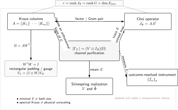
One purification organizes three realizations of the same unread map. Tracing the environment gives the Choi operator, choosing its basis gives a Kraus family, and retaining it gives the complementary output; measuring it adds an outcome-resolved instrument, while rank and minimal realization remain channel invariants.

Gauge Freedom, Padding, and Compression

Mix Kraus families with an isometry

Let $\{K_a\}_{a=1}^{r}$ be a minimal family and let $W:\mathbb C^r\to\mathbb C^m$ satisfy $W^\dagger W=I_r$. Define

$$L_b=\sum_{a=1}^{r}W_{ba}K_a, \qquad b=1,\ldots,m.$$

If $A$ and $B$ are the corresponding Kraus-column matrices, then

$$B=AW^{\mathsf T}, \qquad BB^\dagger =AW^{\mathsf T}W^*A^\dagger =AA^\dagger.$$

Thus $\{L_b\}$ represents the same unread map. For $m=r$, $W$ is unitary and gives a basis rotation. For $m>r$, it is a rectangular isometry that embeds the minimal label space in a larger one. In Stinespring form the same relation is

$$V_L=(I_{\mathrm{out}}\otimes W)V_K.$$

The isometry freedom is necessary, not a nuisance to be removed by naming one favorite Kraus list. It is the precise statement behind the warning that individual Kraus operators are not channel invariants. Standard treatments give equivalent formulations with conjugated coefficient conventions; the declared definition of $W$ decides where the conjugation appears (Kraus 1983; Nielsen and Chuang 2010).

Align padded environment spaces

Two minimal realizations of the same map are related by a unitary on their $r$-dimensional environment supports. Two nonminimal lists can have different lengths, so an operator-by-operator comparison is meaningless until both are embedded in a common space. Append zero Kraus operators or embed each environment isometrically, then solve for the unitary or partial isometry that aligns the occupied supports.

This alignment distinguishes gauge mismatch from physical disagreement. Directly subtracting the first operator in one list from the first in another can report a large discrepancy even when their Choi operators are identical. Conversely, a near unitary match between a few chosen columns does not prove channel equality if discarded columns carry nonnegligible weight.

For approximate comparisons, state both the padding convention and the norm used to compare the common maps. A Procrustes fit on factors is a diagnostic; agreement of $AA^\dagger$ is the invariant test. If environments remain accessible, also state whether the alignment is an allowed change of coordinates or a physically implemented transformation on that record.

Compress product Kraus families

If $\Phi(X)=\sum_aK_aXK_a^\dagger$ acts first and $\Psi(Y)=\sum_bL_bYL_b^\dagger$ acts second, then

$$(\Psi\circ\Phi)(X) =\sum_{a,b}(L_bK_a)X(L_bK_a)^\dagger.$$

The displayed product list has $m_\Phi m_\Psi$ members, but that count is only an upper bound on the composite Choi rank. Form its Kraus-column matrix, determine the rank at the declared tolerance, and factor the resulting Choi operator or use a singular-value factorization. The Audit 2 family below has four products but only two independent directions.

Compression preserves the map only when all nonzero directions are retained. Approximate truncation requires a new physicality check and a task-facing error bound. In particular, retaining the largest columns by norm is not generally equivalent to retaining the leading singular directions, because columns need not be orthogonal. Rank reduction is a structural calculation, not a license to drop inconvenient outcomes.

Measuring the Environment Creates an Instrument

A measurement basis defines branch maps

Projectively measure $E$ in an orthonormal basis $\{\lvert\mu\rangle_E\}$. The outcome operator and branch map are

$$L_\mu = {}_E\!\langle\mu\rvert V =\sum_a\langle\mu\vert a\rangle K_a, \qquad \mathcal I_\mu(\rho)=L_\mu\rho L_\mu^\dagger,$$

with

$$p_\mu=\operatorname{Tr}\mathcal I_\mu(\rho), \qquad \sum_\mu\mathcal I_\mu=\Phi.$$

The conditional state is $\mathcal I_\mu(\rho)/p_\mu$ only when $p_\mu>0$. Keeping the subnormalized branch until its trace has been recorded preserves both the quantum output and the classical probability. General environment measurements can require several operators for one outcome, but the same principle holds: an instrument is additional outcome-resolved structure.

Different instruments can share one unread channel

Changing the measured environment basis coherently mixes the branch operators. Completeness of the basis ensures that their sum still equals $\Phi$, but individual probabilities and conditional states can change. The dephasing and reset audits give explicit pairs: computational and Hadamard environment measurements produce different branch records while agreeing exactly after the record is erased.

This is not a contradiction with Kraus gauge freedom. Gauge freedom states that an unread channel is unchanged under the admissible mixing. Once an environment basis is operationally measured, that choice defines which coherent alternatives are combined before a probability is assigned. The measured basis is then part of the experiment, not disposable notation.

An adversary with coherent access to $E$ can also distinguish dilations that appear identical to a receiver who sees only the system. Questions about complementary information must therefore specify access. Equality of unread maps is sufficient for state propagation on the system, but not for equality of all extended experiments involving the chosen environments.

A spectral family is not automatically an unraveling

Diagonalizing $J_\Phi$ returns orthogonal Hilbert–Schmidt factors. It does not reconstruct which bath observable was monitored, whether any monitoring occurred, or whether the effective map arose from a time-resolved stochastic process. Calling its labels “jumps” adds a physical assertion absent from the matrix factorization.

A licensed unraveling specifies at least a system–environment model, environment preparation, monitoring scheme, temporal resolution, and conditioning rule. Different monitoring schemes can unravel the same master equation or unread channel into different trajectories. Conversely, coarse graining or detector inefficiency can merge distinct microscopic records into one operation (Breuer and Petruccione 2002).

Use spectral Kraus operators for algebraic compression and numerical conversion. Use physically derived measurement operators for event interpretation. If the two coincide, document the derivation that makes them coincide rather than relying on the spectral form itself.

Choose the Realization for the QI Task

Propagation, physicality, and compression

For applying a map to a modest number of states, a short structured Kraus family is often the clearest representation. For certifying complete positivity, imposing trace constraints, or finding the minimal support, the Choi operator is direct. For questions about discarded information, purification, or an accessible auxiliary record, use a Stinespring realization and its complement.

Conversions should be followed by invariant checks appropriate to the task: equality of Choi operators, action on a complete operator basis, TP or TNI completeness, and agreement of the common nonzero spectrum. These checks are stronger than comparing a few named Kraus operators. They also localize failures: a wrong trace usually indicates normalization or subsystem order, while a different Choi factor with the same product often indicates harmless gauge freedom.

Dense storage is not automatically the best computational choice. A rank-$r$ Kraus action can avoid materializing a $(d_{\mathrm{out}}d_{\mathrm{in}})^2$ Choi array, while a Choi factor can expose low rank before repeated simulation. Noise Simulation owns scalable execution choices; the crosswalk here supplies the exact finite object those algorithms must preserve.

Environment access, reset, reuse, and memory

Before choosing a dilation, ask what happens to $E$ after one use. If it is discarded and freshly prepared for every invocation, the one-use channel may be sufficient for the declared context. If it is retained, measured, reused, or initially correlated with the input, additional predictions depend on that record and cannot be recovered from $J_\Phi$ alone.

Reset is an operational assumption, not an algebraic consequence of minimality. Reusing the same auxiliary system can correlate successive outputs even when every isolated marginal resembles the same channel. Likewise, a measured environment creates a classical history that can feed forward into later controls. A process tensor or another multitime model is needed when interventions probe those correlations.

For privacy or error-correction questions, the complement may represent information available outside the logical output. Its basis is gauge dependent, but information quantities invariant under output isometries can still be meaningful. The access model—receiver, adversary, monitored bath, or inaccessible loss port—must accompany the calculation.

Rank does not fix synthesis cost

The ledger below separates exact channel invariants from realization choices and claims that need evidence beyond one channel record.

Quantity or change	Channel invariant	What may change	Required evidence or canonical owner
common minimal rank	$r=\operatorname{rank}J=\operatorname{rank}G$	displayed list length and padded dimension	exact factorization or declared numerical threshold
nonzero Choi/Gram spectrum	same values with the fixed Choi normalization	eigenvectors, phases, and zero multiplicity	spectral decomposition and convention record
TP or TNI condition	$\sum_aK_a^\dagger K_a=I$ or $\preceq I$	matrix coordinates under input-basis changes	formal channel owner and explicit completeness check
Kraus/environment basis rotation	unread map is unchanged for admissible isometries	branch operators, environment matrix entries, and measured probabilities	declared basis and access model
zero padding/isometric embedding	unread map and minimal rank are unchanged	list length and nominal environment dimension	common padded space and occupied-support check
measured environment instrument	unread sum may remain $\Phi$	outcomes, probabilities, and conditional states	specified measurement and instrument record
microscopic bath/synthesis cost claim	not determined by the channel	hardware dimension, coupling, gate count, reset, and approximation cost	device model, compiler, and experimental evidence

Rank gives the smallest pure auxiliary dimension for an exact abstract realization. It neither counts elementary gates nor chooses a native circuit. Two channels with the same $r$ may differ radically in symmetry, locality, controlled-unitary structure, and approximation difficulty. Conversely, an architecture may synthesize a high-rank structured channel cheaply through randomization or reset while a low-rank dense isometry is expensive.

The correct handoff therefore preserves both layers: quote $r$ as a channel invariant, then attach the target gate set, connectivity, error tolerance, ancilla lifecycle, and cost metric for synthesis. The continuity of Stinespring representations gives important analytic control over approximate channels (Kretschmann, Schlingemann, and Werner 2008), but translating that control into resources remains architecture dependent.

Three Reproducible Finite Audits

Audit 1 — One dephasing map, two instruments

Take $p=1/4$ and

$$K_0=\sqrt{\frac34}\,I, \qquad K_1=\sqrt{\frac14}\,Z.$$

The Choi spectrum is $\{3/2,1/2,0,0\}$, its rank is two, and the Bloch-vector contraction is $(r_x,r_y,r_z)\mapsto(r_x/2,r_y/2,r_z)$. Rotating the Kraus-label basis by the Hadamard gives $L_\pm=(K_0\pm K_1)/\sqrt2$. Both families are complete and have the same Choi operator and unread action, but their one-operator branch maps define different instruments.

For $\boldsymbol r=(1/5,-2/5,3/5)$, the rotated probabilities are

$$p_\pm=\frac12\pm\frac{3\sqrt3}{20},$$

while the unread output has Bloch vector $(1/10,-1/5,3/5)$. The branch probabilities retain interference between the original Kraus coordinates; erasing their labels removes that distinction.

Audit 2 — Compress a four-product composition

Compose the $p_1=1/4$ dephasing channel with a $p_2=1/3$ dephasing channel. In the ordered list

$$K_0^{(2)}K_0^{(1)},\quad K_0^{(2)}K_1^{(1)},\quad K_1^{(2)}K_0^{(1)},\quad K_1^{(2)}K_1^{(1)},$$

the four products are proportional to $I,Z,Z,I$ with squared weights $1/2,1/6,1/4,1/12$. The product-column matrix therefore has four columns but rank two. Combining like directions gives the minimal family

$$\sqrt{\frac7{12}}\,I, \qquad \sqrt{\frac5{12}}\,Z.$$

The composite Choi spectrum is $\{7/6,5/6,0,0\}$ and the Bloch contraction is $1/6$ in the $x$ and $y$ directions. Equality of Choi operators, completeness, and action on the Audit 1 input verify that compression changed only the realization.

Audit 3 — A reset channel transfers its input to the environment

Consider

$$\mathcal R(\rho) =\lvert0\rangle\!\langle0\rvert\operatorname{Tr}\rho, \qquad K_0=\lvert0\rangle\!\langle0\rvert, \qquad K_1=\lvert0\rangle\!\langle1\rvert.$$

In the declared output–input ordering,

$$J_{\mathcal R}=\operatorname{diag}(1,1,0,0), \qquad \operatorname{rank}J_{\mathcal R}=2.$$

The Stinespring map sends $\lvert\psi\rangle$ to $\lvert0\rangle_{\mathrm{out}}\lvert\psi\rangle_E$. Hence $V^\dagger V=I$, the unread output is always $\lvert0\rangle\!\langle0\rvert$, and $\widetilde{\mathcal R}(\rho)=\rho$ in the declared basis. On the Audit 1 input, computational-basis environment measurement has probabilities $(4/5,1/5)$; Hadamard-basis measurement has $(3/5,2/5)$. Both instruments sum to the reset channel.

The following dependency-free program performs all three audits with complex matrices and an absolute tolerance of $10^{-12}$. It constructs the Choi and Gram objects, Stinespring outputs and partial traces, and every branch probability rather than inserting the asserted results.

const TOL = 1e-12;

const C = (r, i = 0) => ({ r, i });
const add = (a, b) => C(a.r + b.r, a.i + b.i);
const sub = (a, b) => C(a.r - b.r, a.i - b.i);
const mul = (a, b) => C(a.r * b.r - a.i * b.i, a.r * b.i + a.i * b.r);
const conj = (a) => C(a.r, -a.i);
const scl = (s, a) => C(s * a.r, s * a.i);
const abs = (a) => Math.hypot(a.r, a.i);
const z = () => C(0);

function matrix(rows, cols, f = () => z()) {
  return Array.from({ length: rows }, (_, r) =>
    Array.from({ length: cols }, (_, c) => f(r, c))
  );
}

function eye(n) {
  return matrix(n, n, (r, c) => C(r === c ? 1 : 0));
}

function dagger(a) {
  return matrix(a[0].length, a.length, (r, c) => conj(a[c][r]));
}

function mm(a, b) {
  if (a[0].length !== b.length) throw new Error("matrix shape mismatch");
  return matrix(a.length, b[0].length, (r, c) => {
    let s = z();
    for (let k = 0; k < b.length; k += 1) s = add(s, mul(a[r][k], b[k][c]));
    return s;
  });
}

function plus(a, b) {
  return matrix(a.length, a[0].length, (r, c) => add(a[r][c], b[r][c]));
}

function scale(s, a) {
  return matrix(a.length, a[0].length, (r, c) => scl(s, a[r][c]));
}

function kron(a, b) {
  return matrix(a.length * b.length, a[0].length * b[0].length, (r, c) =>
    mul(a[Math.floor(r / b.length)][Math.floor(c / b[0].length)],
      b[r % b.length][c % b[0].length])
  );
}

function trace(a) {
  let s = z();
  for (let r = 0; r < a.length; r += 1) s = add(s, a[r][r]);
  return s;
}

function outer(v, w) {
  return matrix(v.length, w.length, (r, c) => mul(v[r], conj(w[c])));
}

function vecCol(a) {
  const v = [];
  for (let c = 0; c < a[0].length; c += 1) {
    for (let r = 0; r < a.length; r += 1) v.push(a[r][c]);
  }
  return v;
}

function krausKetOI(a) {
  const dOut = a.length;
  const dIn = a[0].length;
  const column = vecCol(a);
  return Array.from({ length: dOut * dIn }, (_, q) => {
    const out = Math.floor(q / dIn);
    const input = q % dIn;
    return column[input * dOut + out];
  });
}

function choi(kraus) {
  const n = kraus[0].length * kraus[0][0].length;
  let j = matrix(n, n);
  for (const k of kraus) {
    const v = krausKetOI(k);
    j = plus(j, outer(v, v));
  }
  return j;
}

function gram(kraus) {
  return matrix(kraus.length, kraus.length, (a, b) =>
    trace(mm(dagger(kraus[a]), kraus[b]))
  );
}

function krausAction(kraus, rho) {
  let out = matrix(kraus[0].length, kraus[0].length);
  for (const k of kraus) out = plus(out, mm(mm(k, rho), dagger(k)));
  return out;
}

function complete(kraus) {
  let out = matrix(kraus[0][0].length, kraus[0][0].length);
  for (const k of kraus) out = plus(out, mm(dagger(k), k));
  return out;
}

function stinespring(kraus) {
  const dOut = kraus[0].length;
  const dIn = kraus[0][0].length;
  const m = kraus.length;
  return matrix(dOut * m, dIn, (row, col) => {
    const out = Math.floor(row / m);
    const a = row % m;
    return kraus[a][out][col];
  });
}

function traceEnvironment(joint, dOut, dEnv) {
  return matrix(dOut, dOut, (a, b) => {
    let s = z();
    for (let e = 0; e < dEnv; e += 1) s = add(s, joint[a * dEnv + e][b * dEnv + e]);
    return s;
  });
}

function traceOutput(joint, dOut, dEnv) {
  return matrix(dEnv, dEnv, (a, b) => {
    let s = z();
    for (let o = 0; o < dOut; o += 1) s = add(s, joint[o * dEnv + a][o * dEnv + b]);
    return s;
  });
}

function maxDiff(a, b) {
  let d = 0;
  for (let r = 0; r < a.length; r += 1) {
    for (let c = 0; c < a[0].length; c += 1) d = Math.max(d, abs(sub(a[r][c], b[r][c])));
  }
  return d;
}

function check(ok, label) {
  if (!ok) throw new Error(label);
}

function close(x, y, label) {
  check(Math.abs(x - y) <= TOL, `${label}: ${x} != ${y}`);
}

function closeMatrix(a, b, label) {
  check(maxDiff(a, b) <= TOL, label);
}

function closeList(a, b, label) {
  check(a.length === b.length, `${label}: length`);
  for (let q = 0; q < a.length; q += 1) close(a[q], b[q], label);
}

function realHermitianEigenvalues(a) {
  const n = a.length;
  const x = Array.from({ length: n }, (_, r) =>
    Array.from({ length: n }, (_, c) => {
      check(Math.abs(a[r][c].i) <= TOL, "real fixture required");
      close(a[r][c].r, a[c][r].r, "Hermitian fixture");
      return a[r][c].r;
    })
  );
  for (let sweep = 0; sweep < 100 * n * n; sweep += 1) {
    let p = 0;
    let q = 1;
    let largest = 0;
    for (let r = 0; r < n; r += 1) {
      for (let c = r + 1; c < n; c += 1) {
        if (Math.abs(x[r][c]) > largest) {
          largest = Math.abs(x[r][c]);
          p = r;
          q = c;
        }
      }
    }
    if (largest <= TOL) break;
    const angle = 0.5 * Math.atan2(2 * x[p][q], x[q][q] - x[p][p]);
    const cs = Math.cos(angle);
    const sn = Math.sin(angle);
    const pp = cs * cs * x[p][p] - 2 * sn * cs * x[p][q] + sn * sn * x[q][q];
    const qq = sn * sn * x[p][p] + 2 * sn * cs * x[p][q] + cs * cs * x[q][q];
    for (let k = 0; k < n; k += 1) {
      if (k !== p && k !== q) {
        const kp = cs * x[k][p] - sn * x[k][q];
        const kq = sn * x[k][p] + cs * x[k][q];
        x[k][p] = x[p][k] = kp;
        x[k][q] = x[q][k] = kq;
      }
    }
    x[p][p] = pp;
    x[q][q] = qq;
    x[p][q] = x[q][p] = 0;
  }
  return x.map((row, r) => row[r]).sort((a, b) => b - a);
}

function hermitianRank(a) {
  return realHermitianEigenvalues(a).filter((v) => Math.abs(v) > TOL).length;
}

function rhoBloch(x, y, zc) {
  return [
    [C((1 + zc) / 2), C(x / 2, -y / 2)],
    [C(x / 2, y / 2), C((1 - zc) / 2)]
  ];
}

function bloch(rho) {
  return [2 * rho[0][1].r, -2 * rho[0][1].i, rho[0][0].r - rho[1][1].r];
}

function branchProb(k, rho) {
  const p = trace(mm(mm(k, rho), dagger(k)));
  check(Math.abs(p.i) <= TOL, "branch trace not real");
  return p.r;
}

const I = eye(2);
const Z = [[C(1), C(0)], [C(0), C(-1)]];
const H = scale(1 / Math.sqrt(2), [[C(1), C(1)], [C(1), C(-1)]]);
const rho = rhoBloch(1 / 5, -2 / 5, 3 / 5);

const dephasing = [scale(Math.sqrt(3) / 2, I), scale(1 / 2, Z)];
const rotated = [
  scale(1 / Math.sqrt(2), plus(dephasing[0], dephasing[1])),
  scale(1 / Math.sqrt(2), plus(dephasing[0], scale(-1, dephasing[1])))
];
closeMatrix(complete(dephasing), I, "Audit 1 original completeness");
closeMatrix(complete(rotated), I, "Audit 1 rotated completeness");
closeMatrix(mm(dagger(H), H), I, "Audit 1 environment Hadamard");
closeMatrix(choi(dephasing), choi(rotated), "Audit 1 Choi agreement");
closeMatrix(krausAction(dephasing, rho), krausAction(rotated, rho), "Audit 1 action agreement");
closeList(realHermitianEigenvalues(choi(dephasing)), [3 / 2, 1 / 2, 0, 0], "Audit 1 spectrum");
check(hermitianRank(choi(dephasing)) === 2, "Audit 1 rank");
check(hermitianRank(gram(dephasing)) === 2, "Audit 1 Gram rank");
closeList(bloch(krausAction(dephasing, rho)), [1 / 10, -1 / 5, 3 / 5], "Audit 1 Bloch output");
close(branchProb(rotated[0], rho), 1 / 2 + 3 * Math.sqrt(3) / 20, "Audit 1 plus branch");
close(branchProb(rotated[1], rho), 1 / 2 - 3 * Math.sqrt(3) / 20, "Audit 1 minus branch");
close(branchProb(dephasing[0], rho), 3 / 4, "Audit 1 original first branch");
close(branchProb(dephasing[1], rho), 1 / 4, "Audit 1 original second branch");
close(bloch(krausAction(dephasing, rhoBloch(1, 0, 0)))[0], 1 / 2, "Audit 1 contraction");
check(vecCol(I).length === 4, "Audit 1 column vectorization");
closeMatrix(kron(I, I), eye(4), "Audit 1 Kronecker product");

const second = [scale(Math.sqrt(2 / 3), I), scale(Math.sqrt(1 / 3), Z)];
const products = [];
for (const later of second) for (const earlier of dephasing) products.push(mm(later, earlier));
const compressed = [scale(Math.sqrt(7 / 12), I), scale(Math.sqrt(5 / 12), Z)];
check(products.length === 4, "Audit 2 product count");
check(hermitianRank(choi(products)) === 2, "Audit 2 product rank");
check(hermitianRank(gram(products)) === 2, "Audit 2 product Gram rank");
closeMatrix(products[0], scale(Math.sqrt(1 / 2), I), "Audit 2 first weight");
closeMatrix(products[1], scale(Math.sqrt(1 / 6), Z), "Audit 2 second weight");
closeMatrix(products[2], scale(1 / 2, Z), "Audit 2 third weight");
closeMatrix(products[3], scale(Math.sqrt(1 / 12), I), "Audit 2 fourth weight");
closeMatrix(choi(products), choi(compressed), "Audit 2 compressed Choi");
closeMatrix(complete(products), I, "Audit 2 product completeness");
closeMatrix(complete(compressed), I, "Audit 2 compressed completeness");
closeList(realHermitianEigenvalues(choi(compressed)), [7 / 6, 5 / 6, 0, 0], "Audit 2 spectrum");
close(5 / 12, 1 / 4 + 1 / 3 - 2 * (1 / 4) * (1 / 3), "Audit 2 effective probability");
close(bloch(krausAction(compressed, rhoBloch(1, 0, 0)))[0], 1 / 6, "Audit 2 contraction");
closeMatrix(krausAction(products, rho), krausAction(compressed, rho), "Audit 2 action");

const reset = [
  [[C(1), C(0)], [C(0), C(0)]],
  [[C(0), C(1)], [C(0), C(0)]]
];
const resetChoi = [[C(1), C(0), C(0), C(0)], [C(0), C(1), C(0), C(0)],
  [C(0), C(0), C(0), C(0)], [C(0), C(0), C(0), C(0)]];
closeMatrix(choi(reset), resetChoi, "Audit 3 Choi");
check(hermitianRank(choi(reset)) === 2, "Audit 3 rank");
check(hermitianRank(gram(reset)) === 2, "Audit 3 Gram rank");
const V = stinespring(reset);
closeMatrix(mm(dagger(V), V), I, "Audit 3 isometry");
const joint = mm(mm(V, rho), dagger(V));
closeMatrix(traceEnvironment(joint, 2, 2), [[C(1), C(0)], [C(0), C(0)]], "Audit 3 unread reset");
closeMatrix(traceOutput(joint, 2, 2), rho, "Audit 3 complement");
const resetH = [
  scale(1 / Math.sqrt(2), plus(reset[0], reset[1])),
  scale(1 / Math.sqrt(2), plus(reset[0], scale(-1, reset[1])))
];
closeList([branchProb(reset[0], rho), branchProb(reset[1], rho)], [4 / 5, 1 / 5],
  "Audit 3 computational branches");
closeList([branchProb(resetH[0], rho), branchProb(resetH[1], rho)], [3 / 5, 2 / 5],
  "Audit 3 Hadamard branches");
closeMatrix(krausAction(reset, rho), krausAction(resetH, rho), "Audit 3 instrument sums");
closeMatrix(complete(reset), I, "Audit 3 computational completeness");
closeMatrix(complete(resetH), I, "Audit 3 Hadamard completeness");

console.log("Kraus-Choi-Stinespring finite audits: PASS");

Canonical Owners and Common Realization Failures

Use this page when the question is how Kraus columns, Choi factors, and pure-environment Stinespring realizations encode one finite unread map, and when minimal compression or environment access is the point. Use Quantum Channels for QI for the broader representation ledger, conversions to Liouville, process, transfer, and affine forms, and general finite workflow. The formal Kraus, Choi, and Stinespring pages linked above remain the theorem owners.

Comparing Kraus operators one by one. Lists can differ by unitary or rectangular isometric mixing and still define exactly the same map. Compare their Choi products, or pad and align their occupied label spaces before comparing factors.

Calling the displayed list length a rank. Composition and padding routinely create dependent columns. Compute $\operatorname{rank}A$, $\operatorname{rank}J$, or $\operatorname{rank}G$ with an explicit threshold, and distinguish an exact rank from a numerical one.

Dropping a small Choi mode without rechecking the map. Truncation is an approximation, not gauge freedom. Recheck CP, TP or TNI, and a task-facing error; trace-preserving completion may require a principled reconstruction rather than simple deletion.

Treating a spectral factor as a measured event. Choi eigenvectors supply algebraic Kraus coordinates. A physical outcome requires a specified environment measurement or instrument, and a trajectory requires additional dynamical and monitoring assumptions.

Equating a minimal environment with the laboratory bath. Choi rank fixes the smallest pure auxiliary space for one map. It does not infer microscopic modes, reset behavior, correlations across uses, or a native circuit.

Ignoring access when comparing dilations. Environment isometries are invisible after tracing, but not necessarily to an observer who can retain or measure the auxiliary output. State which systems and classical records are accessible before declaring two extended implementations operationally equivalent.

Normalizing branches too early. $\mathcal I_\mu(\rho)$ is subnormalized and its trace is the outcome probability. Save that trace before forming a conditional state, and verify that all branch maps sum to the advertised unread channel.

Inferring memorylessness from a one-use Choi operator. The Choi operator characterizes the declared one-slot map. Environment reuse, initial correlations, drift, and intervention dependence require multitime evidence and a larger operational model.

Exercises

1. Recover a spectral Kraus family

For the $p=1/4$ dephasing channel, factor its Choi operator and verify trace preservation, eigenvalues, and exact rank. State what a numerical calculation must report.

Solution

The Choi operator is $J=(3/4)\lvert I\rangle\!\rangle_{\mathrm{OI}}\langle\!\langle I\rvert_{\mathrm{OI}}+(1/4)\lvert Z\rangle\!\rangle_{\mathrm{OI}}\langle\!\langle Z\rvert_{\mathrm{OI}}$. Since the two Pauli vectors are orthogonal and have squared norm two, its eigenvalues are $3/2,1/2,0,0$. Weighted normalized eigenvectors recover $K_0=\sqrt{3/4}I$ and $K_1=\sqrt{1/4}Z$ by output–input unvectorization. Their completeness sum is $(3/4+1/4)I=I$, so the map is TP, and the exact rank is two. A floating-point result must state its eigenvalue threshold; it may call the rank numerical, but must not turn a small retained mode into an exact zero without an error argument.

2. Compare the Choi and Kraus Gram spectra

For a rectangular Kraus-column matrix $A$, prove that $AA^\dagger$ and $A^\dagger A$ have the same nonzero spectrum, and deduce the common minimal dimension.

Solution

If $A^\dagger Ay=\lambda y$ with $\lambda>0$, then $Ay\ne0$ and $AA^\dagger(Ay)=\lambda(Ay)$. Conversely, $AA^\dagger x=\lambda x$ implies that $A^\dagger x\ne0$ is a $\lambda$ eigenvector of $A^\dagger A$. The maps preserve multiplicities on every positive eigenspace, equivalently giving the squared nonzero singular values of $A$. Hence $\operatorname{rank}(AA^\dagger)=\operatorname{rank}A=\operatorname{rank}(A^\dagger A)=r$. Exactly $r$ independent Kraus columns are necessary and sufficient, and the Schmidt form of the associated purification needs exactly $r$ environment dimensions.

3. Rotate a dephasing instrument

Apply the Hadamard label rotation to the dephasing family and derive the branch probabilities for an input with Bloch component $r_z$. Explain the physical limitation.

Solution

$L_\pm=(K_0\pm K_1)/\sqrt2$ and $\sum_\pm L_\pm\rho L_\pm^\dagger=\sum_aK_a\rho K_a^\dagger$. Moreover, $L_\pm^\dagger L_\pm=I/2\pm(\sqrt3/4)Z$, so $p_\pm=1/2\pm\sqrt3 r_z/4$. At $r_z=3/5$ these become $1/2\pm3\sqrt3/20$. Both effects sum to $I$, rechecking completeness. The rotated and unrotated branch families are different instruments with one unread channel; neither label is a physical detector event unless a corresponding environment measurement has been specified.

4. Compress two composed dephasing maps

Compose dephasing probabilities $p_1=1/4$ and $p_2=1/3$, compress the four products, and check exact rank and TP.

Solution

The two $I$ products have squared weights $(1-p_1)(1-p_2)+p_1p_2=1/2+1/12=7/12$. The two $Z$ products have total weight $(1-p_1)p_2+p_1(1-p_2)=1/4+1/6=5/12$. Thus the minimal family is $\{\sqrt{7/12}I,\sqrt{5/12}Z\}$. Its completeness sum is $I$, its Choi eigenvalues are $7/6$ and $5/6$, and its exact rank is two. The original count four is only a redundant list length; numerical compression would additionally declare a tolerance and recheck TP after truncation.

5. Align minimal and padded realizations

Pad a minimal pair $\{K_0,K_1\}$ to $\{K_0/\sqrt2,K_0/\sqrt2,K_1\}$ and exhibit the environment embedding.

Solution

Use

$$W=\begin{pmatrix}1/\sqrt2&0\\1/\sqrt2&0\\0&1\end{pmatrix}, \qquad W^\dagger W=I_2.$$

Then $L_b=\sum_aW_{ba}K_a$ gives the padded triple, $B=AW^{\mathsf T}$, and $BB^\dagger=AA^\dagger$. The corresponding dilation is $V_L=(I\otimes W)V_K$; its environment is three-dimensional but its occupied support and minimal dimension remain two. A second padded realization must first be embedded in the same ambient space before a unitary alignment is sought. Removing any nonzero direction would require new TP and action checks.

6. Retain and measure the reset environment

For the reset isometry, find the complementary output and the computational- and Hadamard-basis branch probabilities on the audit state.

Solution

$V\lvert\psi\rangle=\lvert0\rangle\lvert\psi\rangle$, so tracing the system gives $\widetilde{\mathcal R}(\rho)=\rho$, while tracing $E$ gives $\lvert0\rangle\!\langle0\rvert$. Computational measurement uses $K_0,K_1$ and reads the diagonal probabilities $(4/5,1/5)$. Hadamard measurement uses $(K_0\pm K_1)/\sqrt2$ and reads $(1\pm r_x)/2=(3/5,2/5)$. In each basis the subnormalized branch maps sum to $\mathcal R$ and their traces sum to one. These outcomes describe the specified environment measurements, not a unique trajectory inherent in the reset channel.

References

• H.-P. Breuer and F. Petruccione, The Theory of Open Quantum Systems, Oxford University Press, Oxford (2002), doi:10.1093/acprof:oso/9780199213900.001.0001.
• M.-D. Choi, “Completely Positive Linear Maps on Complex Matrices,” Linear Algebra and its Applications 10, 285–290 (1975), doi:10.1016/0024-3795(75)90075-0.
• A. S. Holevo, Quantum Systems, Channels, Information: A Mathematical Introduction, De Gruyter, Berlin and Boston (2012), doi:10.1515/9783110273403.
• A. S. Holevo and V. Giovannetti, “Quantum Channels and Their Entropic Characteristics,” Reports on Progress in Physics 75, 046001 (2012), doi:10.1088/0034-4885/75/4/046001.
• A. Jamiołkowski, “Linear Transformations Which Preserve Trace and Positive Semidefiniteness of Operators,” Reports on Mathematical Physics 3, 275–278 (1972), doi:10.1016/0034-4877(72)90011-0.
• K. Kraus, “General State Changes in Quantum Theory,” Annals of Physics 64, 311–335 (1971), doi:10.1016/0003-4916(71)90108-4.
• K. Kraus, States, Effects, and Operations: Fundamental Notions of Quantum Theory, Lecture Notes in Physics 190, Springer-Verlag, Berlin (1983), doi:10.1007/3-540-12732-1.
• D. Kretschmann, D. Schlingemann, and R. F. Werner, “The Information-Disturbance Tradeoff and the Continuity of Stinespring’s Representation,” IEEE Transactions on Information Theory 54, 1708–1717 (2008), doi:10.1109/TIT.2008.917696.
• M. A. Nielsen and I. L. Chuang, Quantum Computation and Quantum Information, 10th anniversary ed., Cambridge University Press, Cambridge (2010), doi:10.1017/CBO9780511976667.
• W. F. Stinespring, “Positive Functions on C*-Algebras,” Proceedings of the American Mathematical Society 6, 211–216 (1955), doi:10.1090/S0002-9939-1955-0069403-4.
• E. C. G. Sudarshan, P. M. Mathews, and J. Rau, “Stochastic Dynamics of Quantum-Mechanical Systems,” Physical Review 121, 920–924 (1961), doi:10.1103/PhysRev.121.920.
• J. Watrous, The Theory of Quantum Information, Cambridge University Press, Cambridge (2018), doi:10.1017/9781316848142.