Leakage and Crosstalk

Leakage and crosstalk invalidate different simplifying boundaries. Leakage moves population or amplitude outside a declared computational sector of one physical system. Crosstalk violates a declared locality or operational-independence model across scheduled regions. This page turns those statements into an auditable record: it constructs a trace-preserving map on the enlarged physical space, extracts the trace-nonincreasing code-survival branch without hiding its probability, separates leakage, seepage, coherent return, loss, and erasure, tests when a two-population recurrence is licensed, and carries leakage state and schedule context through composition. It also gives finite experiments that can reject, but never universally certify, a crosstalk-free model.

Required background. Quantum Channels for QI supplies deterministic and selected-map bookkeeping, Kraus and adjoint representations, and ordered composition. Direct Sums versus Tensor Products supplies the sector-versus-subsystem distinction and block notation used here without rederivation.

Helpful background. Common Noise Models supplies device-facing model cards and the elementary leakage–seepage recurrence. Quantum Instruments supplies the general outcome-record language.

Leakage and Crosstalk Break Different Boundaries

Computational-sector escape

Choose a physical system and a projector $P$ onto the states used to encode the intended computational degrees of freedom. Leakage is population in the complementary sector $Q=I-P$. It is therefore relative to an encoding and a system boundary. The third level of a weakly anharmonic circuit can be leakage for a qubit encoding while remaining an ordinary state in a qutrit computation. Atom or photon loss may instead leave the accepted carrier space altogether.

This definition includes more than a final population count. A coherent pulse can create amplitude between $P$ and $Q$, a later pulse can return that amplitude, and the returned state can carry a logical phase. Conversely, an incoherent process can move population outward and later seep it back without restoring the logical state. Wood and Gambetta formalize average leakage and seepage rates that distinguish these directions, while Wallman, Barnhill, and Emerson show why leakage benchmarking needs observables beyond ordinary trace-preserving qubit models.

Locality and context failure

Crosstalk concerns simultaneous regions rather than alternative sectors. First declare a tensor-factor partition, the operations intended to be local, and any shared resource or joint gate that is allowed. A fixed correlated process across otherwise disjoint regions is a locality failure. A local response that changes when a remote instruction, spectator state, measurement, or reset changes is an operational-independence failure. Either can defeat the declared crosstalk-free model.

The qualification “declared” is essential. Regrouping two coupled components into one region changes the bookkeeping, although it changes no laboratory physics. Likewise, intended entangling gates and licensed common-mode noise can generate correlations without contradicting the model. Sarovar and collaborators formulate crosstalk operationally through locality and conditional independence; Gambetta and collaborators use simultaneous benchmarking to probe addressability under a specified schedule.

Records that keep claims comparable

A portable claim names the computational and leakage projectors, physical basis, tensor order, intended gate or idle, active and idle regions, spectator preparation, control and measurement activity, frame, interval or cycle, leakage classifier, reset policy, accepted shots, acquisition epoch, drift randomization, and held-out contexts. It also states whether the reported object is a full channel, a selected branch, a conditional state, a fitted population law, or an operational statistic.

A bare “leakage rate” does not say whether the input was one basis state or the maximally mixed code state. A bare “crosstalk error” does not say which partition, schedule, spectator, or SPAM assumptions were tested. The purpose of the record is not paperwork: it prevents a parameter measured in one context from being silently reused as a different mathematical object in another.

Freeze the Direct-Sum and Tensor-Product Record

Computational and leakage sectors

For one declared physical system, freeze

$$\mathcal H = \mathcal H_{\mathrm C}\oplus\mathcal H_{\mathrm L}, \qquad P=P_{\mathrm C}, \qquad Q=P_{\mathrm L}=I-P,$$

with finite dimensions

$$d_{\mathrm C}=\operatorname{Tr}P, \qquad d_{\mathrm L}=\operatorname{Tr}Q.$$

The summands are alternative sectors inside one Hilbert space. Operators have blocks such as $PUP$, $PUQ$, $QUP$, and $QUQ$; the off-diagonal blocks move amplitude between sectors. The direct sum alone neither forbids coherence across sectors nor turns the sectors into separately addressable parties. Superselection, measurement backaction, and controllability are additional physical statements.

Scheduled tensor factors and spectators

Distinct regions present at the same time use tensor factors:

$$\mathcal H_{\mathrm{device}} = \bigotimes_r \left( \mathcal H_{\mathrm C,r}\oplus \mathcal H_{\mathrm L,r} \right).$$

The inner direct sum says that region $r$ may occupy a computational or leakage sector. The outer tensor product says that all declared regions coexist. This arrangement allows, for example, leakage in region $A$ to mediate a phase on spectator $B$. It does not imply that the complement of a many-qubit logical code factorizes into independent leakage subsystems; a code-space complement can contain collective states with no preferred local decomposition.

The spectator record specifies its preparation, whether it is idle or driven, whether it is measured or reset, and whether a hidden state persists between intervals. Without that information, averaging over the spectator can turn a coherent conditional rotation into an apparent stochastic channel whose repetition law is wrong.

Context, frame, and measurement record

The schedule fixes when operations overlap and which frame defines local axes. A virtual frame change, a microwave pulse, a measurement tone, and an active reset can all alter the effective map experienced elsewhere. Record the order rather than treating simultaneous labels as an unordered set. Retain timestamps and calibration epochs so that slow drift can be separated from deliberately varied context.

The measurement record must say whether a sector flag was actually read, ignored after being read, or never coupled to a detector. Those three interventions can have different quantum backaction. The boundary diagram keeps the direct-sum, tensor-product, flag, and persistence distinctions visible.

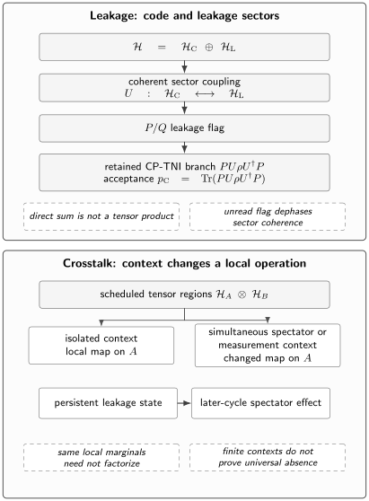
Leakage crosses a direct-sum sector boundary; crosstalk violates a declared tensor-region locality or independence boundary. A sector flag changes coherent return, and a persistent leakage state can affect later scheduled regions.

Full-Space Maps and Code-Survival Branches

CPTP evolution on the full space

Let $\mathcal E$ be completely positive and trace preserving on the declared full physical space. For a Kraus family,

$$\mathcal E(\rho) = \sum_\alpha K_\alpha\rho K_\alpha^\dagger, \qquad \sum_\alpha K_\alpha^\dagger K_\alpha=I.$$

Trace preservation belongs to the enlarged boundary. Projecting the result back into $\mathcal H_{\mathrm C}$ can lose trace because some probability remains in $\mathcal H_{\mathrm L}$. Calling the projected object an ordinary qubit channel erases precisely the event being modeled.

A full-space description also retains cross-sector coherence and leaked-sector state. Those variables determine whether later evolution returns amplitude, randomizes a logical phase, or influences spectators. The general representation and physicality theorems remain at Quantum Channels for QI; here the full map is the bookkeeping object needed for leakage-aware composition.

The trace-nonincreasing retained branch

For any operator $\rho$, define

$$\mathcal C_{\mathcal E}(\rho) := P\,\mathcal E(P\rho P)\,P, \qquad a_{\mathcal E}(\rho) := \operatorname{Tr}\mathcal C_{\mathcal E}(\rho).$$

The retained map is completely positive and trace nonincreasing. For a normalized code-supported input,

$$p_{\mathrm L}(\rho) := \operatorname{Tr}\!\left[Q\mathcal E(\rho)\right] =1-a_{\mathcal E}(\rho).$$

Conditioning on acceptance gives

$$\rho_{\mathrm C\mid\mathrm{acc}} = \frac{\mathcal C_{\mathcal E}(\rho)} {\operatorname{Tr}\mathcal C_{\mathcal E}(\rho)},$$

only when the denominator is nonzero. This normalization is generally nonlinear and is not a channel. For

$$K=\begin{pmatrix}1&0\\0&1/\sqrt2\end{pmatrix},$$

normalizing $K(I/2)K^\dagger$ gives $\operatorname{diag}(2/3,1/3)$. Equally mixing the separately normalized outputs from $\lvert0\rangle\langle0\rvert$ and $\lvert1\rangle\langle1\rvert$ gives $I/2$. Their trace distance is $1/6$. Thus a simulation must carry both the subnormalized branch and its probability until the physical conditioning step.

Leakage, seepage, and worst-case diagnostics

Wood and Gambetta’s sector averages are

$$\begin{aligned} L_1(\mathcal E) &= \operatorname{Tr}\!\left[ Q\mathcal E\!\left(\frac{P}{d_{\mathrm C}}\right) \right] = \frac1{d_{\mathrm C}} \sum_\alpha\left\|QK_\alpha P\right\|_{\mathrm F}^2,\\ L_2(\mathcal E) &= \operatorname{Tr}\!\left[ P\mathcal E\!\left(\frac{Q}{d_{\mathrm L}}\right) \right] = \frac1{d_{\mathrm L}} \sum_\alpha\left\|PK_\alpha Q\right\|_{\mathrm F}^2. \end{aligned}$$

$L_1$ averages escape over the maximally mixed computational sector; $L_2$ averages return over the maximally mixed leakage sector. Neither is automatically a particular preparation’s probability. The worst one-use escape over code-supported density operators is

$$L_{\max}(\mathcal E) := \max_{\substack{\rho=P\rho P,\ \rho\succeq0\\ \operatorname{Tr}\rho=1}} \operatorname{Tr}\!\left[Q\mathcal E(\rho)\right] = \lambda_{\max}\!\left[P\mathcal E^\dagger(Q)P\right].$$

For a unitary $U$ on the full space,

$$L_{\max}(U)=\left\|QUP\right\|_{\mathrm{op}}^2.$$

Only a unital full-space channel licenses $d_{\mathrm C}L_1=d_{\mathrm L}L_2$. A reset, thermalization, loss process, or selected branch is generally nonunital.

Leakage, Seepage, Loss, and Erasure

Distinct events and information records

Leakage is occupancy of the declared $Q$ sector. Seepage is transfer from $Q$ back to $P$; it need not recover the original logical state. Loss removes a carrier or excitation from the accepted system boundary. Erasure supplies a classical record that locates an error, with declared false-positive and false-negative behavior. Bennett, DiVincenzo, and Smolin’s erasure-channel capacities rely on this flagged distinction, not merely on missing amplitude.

A vacuum or orthogonal erasure flag can be included in an enlarged trace-preserving output space. Discarding the flag gives a trace-decreasing survival operation. A higher energy level is not automatically loss, and a detected higher-level signature is not automatically a perfect erasure. The formal channel distinctions and bosonic attenuation models belong to Erasure and Loss Channels.

Average and state-resolved rates

State-resolved leakage asks what escaped from a specified preparation. The average $L_1$ asks the same question for $P/d_{\mathrm C}$. Worst-case leakage optimizes over all code density operators. These can differ substantially when only one logical direction couples to an unwanted level. Wallman, Barnhill, and Emerson develop robust leakage characterization while emphasizing that survival and population observables must be interpreted with the sequence and SPAM model.

The eleven operational quantities used throughout the page are summarized below. Every row names the conditioning record because the same symbol measured under another schedule or classifier can denote another estimand.

quantity	symbol	defining expression or estimator	conditioning record	allowed range or license	common failure
State-resolved leakage	$p_{\mathrm L}(\rho)$	$\operatorname{Tr}[Q\mathcal E(\rho)]$	input $\rho$, full map, interval	$[0,1]$ for normalized code input	confused with $L_1$
Code acceptance	$a_{\mathcal E}(\rho)$	$\operatorname{Tr}\mathcal C_{\mathcal E}(\rho)$	accepted branch and input	$[0,1]$; retain with conditional state	normalization hides rejected shots
Wood–Gambetta average leakage	$L_1$	$\operatorname{Tr}[Q\mathcal E(P/d_{\mathrm C})]$	code sector and averaging state	$[0,1]$	reported as every state’s leakage
Wood–Gambetta average seepage	$L_2$	$\operatorname{Tr}[P\mathcal E(Q/d_{\mathrm L})]$	leakage sector and averaging state	$[0,1]$	interpreted as logical recovery
Worst-case leakage	$L_{\max}$	$\lambda_{\max}[P\mathcal E^\dagger(Q)P]$	code-supported density operators	$[0,1]$	Frobenius norm substituted for operator norm
Coherent leakage	$C_{\mathrm L}$	$\lVert\mathcal E(\rho)-\Delta(\mathcal E(\rho))\rVert_1$	state, sector split, unread map	$0\leq C_{\mathrm L}\leq2\sqrt{p_{\mathrm C}p_{\mathrm L}}$	called a probability or fidelity
Ideal leakage-flag probability	$p_{\mathrm{flag}}$	$p_{\mathrm L}$	projective sector flag after the map	exact only for the ideal instrument	measurement backaction ignored
Imperfect leakage-flag probability	$p_{\mathrm{flag}}$	$(1-f_{\mathrm n})p_{\mathrm L}+f_{\mathrm p}(1-p_{\mathrm L})$	calibrated $f_{\mathrm p},f_{\mathrm n}$ and epoch	inversion needs $1-f_{\mathrm n}-f_{\mathrm p}\neq0$	unstable or out-of-range inversion
Population recurrence eigenmode	$q$	$1-L_1-L_2$	one closed, fixed cycle	$[-1,1]$ for stochastic rates	reused after context or hidden state changes
Context discrepancy	$\delta_A(c,c')$	$\tfrac12\lVert\mathcal E_{A\mid c}-\mathcal E_{A\mid c'}\rVert_\diamond$	fixed local record, varied remote context	needs licensed reconstruction or bound	treated as directly observed
Connected XX witness	$C_{XX}$	$\langle X_AX_B\rangle-\langle X_A\rangle\langle X_B\rangle$	declared partition and trusted product SPAM	$[-1,1]$ by Cauchy–Schwarz; fixture gives $0.36$	correlation alone called crosstalk

Ideal and imperfect leakage flags

An ideal sector measurement after $\mathcal E$ has operations

$$\mathcal I_{\mathrm C}(\rho)=P\mathcal E(\rho)P, \qquad \mathcal I_{\mathrm L}(\rho)=Q\mathcal E(\rho)Q.$$

Ignoring the recorded outcome produces

$$\mathcal I_{\mathrm C}+\mathcal I_{\mathrm L} = \Delta\circ\mathcal E, \qquad \Delta(X)=PXP+QXQ,$$

not $\mathcal E$ when cross-sector coherence exists. Reading and discarding a flag can therefore suppress later coherent return. Varbanov and collaborators demonstrate leakage detection in a transmon surface-code setting, but the detector’s performance and backaction are platform- and protocol-qualified.

For false-negative probability $f_{\mathrm n}$ and false-positive probability $f_{\mathrm p}$,

$$p_{\mathrm{flag}} =(1-f_{\mathrm n})p_{\mathrm L} +f_{\mathrm p}(1-p_{\mathrm L}), \qquad p_{\mathrm L} = \frac{p_{\mathrm{flag}}-f_{\mathrm p}} {1-f_{\mathrm n}-f_{\mathrm p}}.$$

The inversion requires transferable calibration and physical-range checks. At $f_{\mathrm n}+f_{\mathrm p}=1$ the flag contains no information about leakage; a small denominator amplifies uncertainty.

The following ledger separates the full process, selected branches, coarse-grained laws, and locality models before any of them is composed:

model or object	physical space and record	map character	structure retained	licensed prediction	principal falsifier
Full-space CPTP process	$\mathcal H_{\mathrm C}\oplus\mathcal H_{\mathrm L}$ and full schedule	linear CPTP	populations, coherence, leaked state	unconditional physical output	trace loss or failed holdout
Retained CP-TNI branch and normalized conditional state	code projector and acceptance event	linear CP-TNI branch; nonlinear normalization	survival probability plus accepted state	accepted-shot statistics	probability discarded or mixture law violated
Loss or flagged-erasure model	enlarged carrier or orthogonal flag space	CPTP with flag, or CP-TNI survival	carrier absence and record	located loss or survival	uncalibrated or missing flag
Coherent and block-dephased leakage models	direct-sum sectors and measurement intervention	unitary/full CPTP versus $\Delta$-interrupted CPTP	cross-sector phase versus populations only	reversal and interference	indistinguishable pulse/hold predictions fail
Two-population leakage–seepage law	closed sector populations for one cycle	stochastic $2\times2$ recurrence	$p_{\mathrm C},p_{\mathrm L}$ only	fixed point and one real mode	state, context, history, or residual structure
Crosstalk-free scheduled tensor product	declared regions and allowed local contexts	tensor product of local maps	regional local state	simultaneous layer from local factors	locality or conditional-independence failure
Context-conditioned reduced channel	product spectator state and remote context	reduced CPTP map when assumptions hold	local response by context	context discrepancy	initial correlation or history dependence
Fixed correlated-ZZ Pauli channel	two declared regions and joint error probability	joint CPTP Pauli channel	correlated parity action	local and joint Pauli moments	SPAM-bounded witness disagrees

Coherent Leakage and Transient Logical Error

Operator blocks and a coherence metric

Block dephasing removes only coherence between the declared sectors. Define the state-resolved quantity, with no factor of $1/2$,

$$C_{\mathrm L}(\mathcal E\mid\rho) := \left\| \mathcal E(\rho)-\Delta(\mathcal E(\rho)) \right\|_1.$$

For a normalized output with sector populations $p_{\mathrm C}$ and $p_{\mathrm L}$, positivity gives

$$0\leq C_{\mathrm L} \leq2\sqrt{p_{\mathrm C}p_{\mathrm L}} \leq1.$$

The quantity detects cross-sector coherence. It is neither a probability nor a fidelity, and its value depends on the declared sector split. Aliferis and Terhal’s treatment of coherent local leakage faults explains why coherent return and leakage-reduction operations matter to fault-tolerance analysis; this page stops at the physical-space diagnostic rather than deriving a threshold theorem.

One coupled code state

Use the ordered qutrit basis $(\lvert0\rangle,\lvert1\rangle,\lvert\ell\rangle)$ and

$$\begin{aligned} U_\theta\lvert0\rangle&=\lvert0\rangle,\\ U_\theta\lvert1\rangle&=\cos\theta\lvert1\rangle+\sin\theta\lvert\ell\rangle,\\ U_\theta\lvert\ell\rangle&=-\sin\theta\lvert1\rangle+\cos\theta\lvert\ell\rangle. \end{aligned}$$

For input $\lvert1\rangle$, the one-pulse state leakage is $\sin^2\theta$ and

$$C_{\mathrm L}(U_\theta\mid\lvert1\rangle\langle1\rvert) =\lvert\sin2\theta\rvert.$$

Only one of the two computational basis states couples, so

$$L_1(U_\theta)=\frac{\sin^2\theta}{2}, \qquad L_2(U_\theta)=L_{\max}(U_\theta)=\sin^2\theta.$$

The equality $2L_1=L_2$ is the unital dimension balance with $d_{\mathrm C}=2$ and $d_{\mathrm L}=1$, not a generic leakage law. Chen and collaborators measured state leakage and its suppression in a superconducting qubit; their platform result illustrates why the preparation and pulse sequence belong beside the number.

At $\theta=0.2$, one-pulse state leakage is $0.039469502998557456$, whereas $L_1=0.019734751499278728$. Also $L_2=L_{\max}=0.039469502998557456$ and $C_{\mathrm L}=0.3894183423086505$. Two coherent pulses give $\sin^2(2\theta)=0.1516466453264173$. Inserting $\Delta$ between pulses gives $2\sin^2\theta\cos^2\theta=0.07582332266320864$. The latter is not the absorbing formula $1-(1-\sin^2\theta)^2$, because this unitary permits seepage.

Hidden phase with zero final leakage

Final population cannot reveal every excursion. Let $S$ swap $\lvert1\rangle$ and $\lvert\ell\rangle$ while fixing $\lvert0\rangle$, and let

$$V_\varphi=P+e^{i\varphi}Q.$$

Then $SV_\varphi S$ returns every code input to the code sector, so its final leakage is zero, but its code restriction is

$$P(SV_\varphi S)P = \operatorname{diag}(1,e^{i\varphi}).$$

A superposition therefore acquires a logical relative phase through a transient leakage path. Population measurements before and after the complete sequence miss it; an interference measurement reveals it. A sector measurement inserted during the excursion also changes the process by destroying cross-sector coherence. Motzoi and collaborators’ derivative-shaped control pulses are a platform-specific example of suppressing coherent population transfer, not a universal guarantee that final population certifies logical accuracy.

Two-Population Dynamics and Its License

The leakage–seepage recurrence

When one fixed cycle closes on the two sector populations, write

$$\begin{pmatrix} p_{\mathrm C,n+1}\\ p_{\mathrm L,n+1} \end{pmatrix} = \begin{pmatrix} 1-L_1&L_2\\ L_1&1-L_2 \end{pmatrix} \begin{pmatrix} p_{\mathrm C,n}\\ p_{\mathrm L,n} \end{pmatrix}.$$

Equivalently,

$$p_{\mathrm L,n+1} = L_1+(1-L_1-L_2)p_{\mathrm L,n}.$$

This law is a coarse-grained model, not the definition of leakage. Its columns sum to one and its entries are nonnegative when $0\leq L_1,L_2\leq1$. Wood and Gambetta use this leakage–seepage structure to interpret repeated randomized sequences; the translation to another experiment still requires its closure assumptions.

Fixed point, decay mode, and edge cases

For fixed rates with $L_1+L_2>0$, define

$$q=1-L_1-L_2, \qquad p_{\mathrm L}^{(\infty)} = \frac{L_1}{L_1+L_2}.$$

Then

$$p_{\mathrm L,n} = p_{\mathrm L}^{(\infty)} +q^n\left( p_{\mathrm L,0}-p_{\mathrm L}^{(\infty)} \right).$$

If $L_1=L_2=0$, every initial population is stationary and the displayed ratio is undefined. If $L_1+L_2=1$, then $q=0$ and the fixed population is reached in one cycle. If $1<L_1+L_2<2$, negative $q$ gives alternating convergence. The endpoint $L_1=L_2=1$ has $q=-1$ and produces a period-two swap, not convergence.

For $L_1=0.02$, $L_2=0.18$, $p_{\mathrm L,0}=0$, $f_{\mathrm p}=0.01$, and $f_{\mathrm n}=0.05$, the complete fixture is:

cycle $n$	$q^n$	$p_{\mathrm C,n}$	$p_{\mathrm L,n}$	ideal flag probability	imperfect flag probability	$p_{\mathrm L}^{(\infty)}-p_{\mathrm L,n}$
$0$	$1$	$1$	$0$	$0$	$0.01$	$0.1$
$1$	$0.8$	$0.98$	$0.02$	$0.02$	$0.0288$	$0.08$
$2$	$0.64$	$0.964$	$0.036$	$0.036$	$0.04384$	$0.064$
$5$	$0.32768$	$0.932768$	$0.067232$	$0.067232$	$0.07319808$	$0.032768$
$10$	$0.1073741824$	$0.91073741824$	$0.08926258176$	$0.08926258176$	$0.0939068268544$	$0.01073741824$

An explicit qutrit realization is

$$\begin{aligned} K_0&=\sqrt{0.98}\,P+\sqrt{0.82}\,Q,\\ K_1&=\sqrt{0.02}\,\lvert\ell\rangle\langle0\rvert, &K_2&=\sqrt{0.02}\,\lvert\ell\rangle\langle1\rvert,\\ K_3&=\sqrt{0.09}\,\lvert0\rangle\langle\ell\rvert, &K_4&=\sqrt{0.09}\,\lvert1\rangle\langle\ell\rvert. \end{aligned}$$

It satisfies $\sum_jK_j^\dagger K_j=I$, has $L_1=0.02$ and $L_2=0.18$, and is nonunital. Thus the unital dimension-balance identity is deliberately unavailable.

When the scalar law fails

The recurrence is licensed only when one fixed map or cycle induces a closed two-population dynamics; cross-sector coherence is absent at the composition boundary or proved not to feed either next population; the leaked-sector state has the return behavior represented by one $L_2$; and the rates do not depend on logical state, leakage level, history, schedule, measurement backaction, or epoch.

Oscillations can be compatible with a negative real $q$, so oscillation alone is not a falsifier. Reject the one-mode law when oscillations are inconsistent with a single real $q^n$, when residuals are structured, autocorrelated, or multiexponential, or when rates change with preparation, context, order, or hold time. McEwen and collaborators observed persistent leakage-mediated correlated errors and studied removal strategies in superconducting error correction; that result motivates retaining hidden state but does not make one persistence time universal.

Crosstalk as Locality or Independence Failure

A factorized scheduled-region model

Relative to a declared partition and allowed local contexts, the simplest Markovian crosstalk-free model is

$$\mathcal E_{\boldsymbol s}^{\mathrm{free}} = \bigotimes_r\mathcal E_{r,s_r},$$

where $s_r$ is the intended local instruction. Every licensed shared resource, frame, feedforward path, or joint operation must already be inside the regional or context record. A process that acts jointly across declared disjoint regions during a layer with no intended joint operation violates locality, even if the same joint process occurs in every tested context.

Murali and collaborators show how schedule and mapping choices can mitigate measured crosstalk on a particular class of processors. Such compilation is an intervention after a model is established; Error-Aware Compilation owns the general scheduling and placement response.

An operational conditional-independence test

For two regions and a fixed product spectator preparation $\sigma_B$, define

$$\mathcal E_{A\mid s_B,\sigma_B}(\rho_A) := \operatorname{Tr}_B \mathcal E_{s_A,s_B} \left(\rho_A\otimes\sigma_B\right).$$

Changing the remote instruction, spectator state, measurement activity, or reset while holding the intended local record fixed tests context dependence. A model-level discrepancy may be written

$$\delta_A(c,c') := \frac12 \left\| \mathcal E_{A\mid c}-\mathcal E_{A\mid c'} \right\|_\diamond,$$

although this distance is not directly observed without a licensed reconstruction or bound. Sarovar and collaborators’ symmetric no-crosstalk conditions are

$$P(R_A\mid S_A,S_B,R_B)=P(R_A\mid S_A), \qquad P(R_B\mid S_A,S_B,R_A)=P(R_B\mid S_B).$$

Failure of either a locality relation or the relevant conditional independence is evidence against the declared free model. Context dependence witnesses independence failure; it is not required to establish a locality violation by an accepted joint process.

Gauge, drift, and boundary caveats

Initial correlations can prevent a state-independent reduced channel on $A$, and memory can make the response depend on earlier interventions. Do not force either case into one fixed local channel. Ordinary observed correlation is also insufficient: intended entanglement, correlated inputs, licensed common-mode noise, or correlated SPAM can create correlations without device crosstalk.

Gate-set estimates carry gauge freedom. Compare observed probabilities, gauge-invariant distances, or jointly gauge-fixed models rather than interpreting one gauge-dependent generator coefficient as a physical rate. Rudinger and collaborators’ context-dependence protocol explicitly separates context tests from drift, while their simultaneous gate-set-tomography experiment demonstrates a gauge-aware route under stated model assumptions. Randomize or interleave contexts, retain timestamps, and use same-epoch controls so that drift is not relabeled as crosstalk.

Physical and Operational Crosstalk Models

Control-path and Hamiltonian mechanisms

Candidate mechanisms include control-line pickup, spectral spillover, frequency crowding, AC Stark shifts, calibration cross-dependence, residual $ZZ$, exchange, and shared-mode coupling. A Hamiltonian model can predict coherent spectator-state-dependent rotations, but a fitted rotation does not uniquely identify its microscopic origin. Pulse amplitude, detuning, duration, echo placement, and simultaneous-drive scans help distinguish hypotheses.

Sheldon and collaborators give a systematic cross-resonance tuning procedure that addresses one residual-interaction setting. Motzoi and collaborators give a leakage-suppressing pulse construction for weak anharmonicity. Both are valuable mechanism-qualified examples; neither supplies a platform-independent crosstalk magnitude or a universal cure. Pulse-Level Control owns control synthesis and calibration methods.

Shared dissipation, measurement, and leakage mediation

Crosstalk need not be coherent. Shared baths can correlate relaxation or dephasing. Measurement resonators, amplifiers, classical discrimination paths, and reset pulses can alter another region’s state or record. Leakage can change dispersive shifts, move through coupled hardware, persist across cycles, and mediate delayed spectator phases. Heating, quasiparticles, or another common disturbance can produce temporal as well as spatial correlations.

The diagnostic must vary the feature that distinguishes the models: spectator state for a conditional Hamiltonian, measurement activity for readout coupling, hold time for persistence, and reset policy for a hidden leakage state. Conditioning only on accepted computational shots can erase evidence while changing the logical estimand. Noise Simulation owns scalable multilevel and correlated propagation once the state and event schedule have been selected.

Residual ZZ and correlated-ZZ fixtures

Freeze the convention

$$U_{ZZ}(\phi) := \exp\!\left(-\frac{i\phi}{2}Z_AZ_B\right).$$

A spectator in a $Z_B$ eigenstate produces a target $Z_A$ rotation by $+\phi$ or $-\phi$. Averaging equally over the signs gives one-interval target coherence $\cos\phi$. If one hidden sign persists through $m$ intervals, the ensemble coherence is $\cos(m\phi)$. If the spectator is independently reset and reprepared in the equal $Z$ mixture before every interval, it is $(\cos\phi)^m$. Reset to a known fixed eigenstate instead gives a deterministic coherent rotation.

At $\phi=0.12$ and $m=8$,

$$\cos\phi=0.9928086358538663, \qquad p_Z=\frac{1-\cos\phi}{2}=0.003595682073066875,$$

while the static-sign coherence is $0.5735199860724567$ and the independent-reset coherence is $0.9438964863182283$. The effective $p_Z$ belongs only to the one-interval equal-sign unread average; it is neither the Hamiltonian coupling nor permission to redraw a persistent sign independently.

A distinct stochastic fixture is

$$\mathcal Z_{AB,p}(\rho) =(1-p)\rho+pZ_AZ_B\rho Z_AZ_B.$$

On $\lvert++\rangle$, $\langle X_A\rangle=\langle X_B\rangle=1-2p$ and $\langle X_AX_B\rangle=1$. At $p=0.1$, the product of local marginals is $0.64$, whereas the joint value is $1$, giving connected witness $0.36$. Across declared disjoint regions with no intended joint operation, this fixed channel is a locality violation and therefore crosstalk under the Sarovar definition. That conclusion from this witness additionally requires trusted product preparation and readout, or explicit SPAM bounds. The fixture does not establish context dependence because no context was varied.

Composition with Leakage State and Schedule Context

Preserve the hidden leakage state

A normalized code state plus one survival scalar cannot predict coherent return, leakage-level-dependent phases, or a later spectator error. Retain the full density operator whenever feasible. A validated hybrid alternative may retain the computational density block, leakage level or leakage-sector block, cross-sector coherence when relevant, schedule context, flag record, reset state, and epoch.

The minimal state depends on the next question. A population-only recurrence can be adequate for a measurement that fully dephases sectors after each cycle. It is inadequate for the $U_\theta$ reversal experiment. A single leakage bit can be adequate when all leaked states share the same return and spectator action; it fails when different unwanted levels have different lifetimes or dispersive shifts.

Compose schedule-conditioned channels

Compose full-space maps right to left in the actual schedule. Only project, dephase, measure, reset, or coarse-grain where an intervention or accepted approximation does so. A context-indexed family of one-time channels does not automatically define a context-independent repeatable process: the next map may depend on the current leakage state, remote activity, measurement record, and history.

For scheduled contexts $c_1,\ldots,c_m$ and no intermediate observation, the prediction is

$$\rho_m = \mathcal E_{c_m}\circ\cdots\circ \mathcal E_{c_2}\circ\mathcal E_{c_1}(\rho_0).$$

Replacing this expression by powers of an averaged qubit channel is a new model claim. It requires evidence that hidden states reset or become irrelevant and that the averaging law is stable under repetition.

Reset, flag, and mitigation interventions

A flag produces an instrument with branch probabilities; a reset is a channel conditioned on a declared record; postselection changes the accepted ensemble. Preserve these distinctions in the composition ledger summarized above. Report attempts per accepted result, false flags, reset failures, and whether conditioning changes the target estimand.

Flags, resets, compilation, and leakage-reduction units are interventions, not relabelings of the original channel. McEwen and collaborators study reset-based removal of persistent leakage; Aliferis and Terhal analyze leakage-reduction scope in fault-tolerant constructions. Why Quantum Error Correction Is Possible owns the logical protection boundary.

Experiments That Distinguish the Models

Leakage preparations, holds, and returns

Prepare computational basis states and superpositions, and prepare accessible leakage levels when the hardware permits. Scan pulse amplitude and duration to expose coherent oscillation; vary a hold interval to measure return and persistence; use reversal or interference sequences to separate coherent excursion from block-dephased transfer. Measure state-resolved leakage, average over a declared code ensemble, and condition logical observables on the flag record without losing the acceptance probability.

Chen and collaborators combine leakage-sensitive measurements with suppression in a superconducting qubit. Varbanov and collaborators calibrate leakage detection for a surface-code setting. McEwen and collaborators expose multi-cycle leakage persistence and correlated consequences. These experiments motivate the menu; their numbers remain tied to their devices, controls, and readout models.

Crosstalk contexts and spectator tomography

Compare isolated and simultaneous operations while interleaving their acquisition. Vary spectator $Z$ eigenstates, superpositions, active or idle status, reset, and readout. Change spatial separation and schedule overlap. Amplify a suspected Hamiltonian over repeated intervals and add echo variants. Measure both local and connected observables, and where justified perform simultaneous tomography or benchmarking.

Gambetta and collaborators’ simultaneous randomized benchmarking probes addressability, Rudinger and collaborators’ simultaneous gate-set tomography estimates context-dependent operations with gauge control, and Murali and collaborators connect measured crosstalk to scheduling choices. Each protocol tests a specified layer and model; none alone covers all preparations, depths, or epochs.

Holdouts, falsifiers, and absence claims

Fit on only part of the preparations, depths, contexts, spectator states, and dates. Hold out unused combinations and test predicted populations, coherences, flag rates, and connected observables with propagated SPAM and sampling uncertainty. Randomization across time distinguishes deliberately varied context from drift. Device Characterization owns general model selection, uncertainty, and gauge-aware inference.

Do not rescue a scalar fit when data show state-dependent rates, oscillations inconsistent with one real $q^n$ mode, cross-sector interference, several return times, structured or autocorrelated residuals, multiexponential decay, context-dependent $L_1$ or $L_2$, history or order effects, correlated spectator observables, classifier drift, or held-out failure. Rudinger’s context protocol is especially useful here because it pairs varied settings with drift controls.

Failure to detect crosstalk is not proof of its universal absence. State the tested regions, settings, schedules, preparations, measurements, time window, statistical power, SPAM assumptions, and epoch. The strongest warranted conclusion is that no violation above a stated sensitivity was found within that domain.

Three Reproducible Finite Audits

Audit 1 — Qutrit leakage, coherence, and flags

The audit constructs $U_{0.2}$ and verifies unitarity. The two Kraus operators of the ideal sector instrument are $K_{\mathrm C}=PU_\theta$ and $K_{\mathrm L}=QU_\theta$, whose effects sum to $I$. The four blocks $PUP$, $PUQ$, $QUP$, and $QUQ$ are not four Kraus operators of that same instrument. The calculation independently recovers the state leakage, $L_1$, $L_2$, $L_{\max}$, $C_{\mathrm L}$, coherent and block-dephased two-pulse values, and the zero-final-leakage phase counterexample. It also verifies the $1/6$ postselection nonlinearity.

Audit 2 — Population law and persistence

The five-Kraus qutrit channel is checked for completeness, its projector-trace and Frobenius definitions both give $L_1=0.02$ and $L_2=0.18$, and its failure of unitality is explicit. Direct channel iteration and the closed form reproduce all five rows of the recurrence table, including imperfect flags and their inversion. Separate fixtures test $q=0$, alternating convergence for negative $q$, and the $q=-1$ period-two endpoint.

Audit 3 — Static, reset, and correlated ZZ

The final audit builds $U_{ZZ}(0.12)$, compares a persistent spectator sign with an independent equal-sign reset before each interval, and recovers both coherence laws. It then propagates $\lvert++\rangle$ through the separate correlated Pauli channel and checks the local, joint, and connected $X$ observables. The connected witness is interpreted only under the declared partition and trusted product SPAM; the program does not manufacture a context test that was not performed.

"use strict";

const tolerance = 1e-12;
const assert = (condition, message) => {
  if (!condition) throw new Error(message);
};
const close = (actual, expected, message) => {
  assert(Math.abs(actual - expected) <= tolerance, `${message}: ${actual} != ${expected}`);
};
const z = (re = 0, im = 0) => [re, im];
const add = ([ar, ai], [br, bi]) => [ar + br, ai + bi];
const sub = ([ar, ai], [br, bi]) => [ar - br, ai - bi];
const mul = ([ar, ai], [br, bi]) => [ar * br - ai * bi, ar * bi + ai * br];
const conj = ([re, im]) => [re, -im];
const scl = ([re, im], value) => [re * value, im * value];
const abs2 = ([re, im]) => re * re + im * im;
const cis = (angle) => [Math.cos(angle), Math.sin(angle)];
const zeros = (rows, columns) => Array.from(
  { length: rows },
  () => Array.from({ length: columns }, () => z()),
);
const real = (matrix) => matrix.map((row) => row.map((value) => z(value)));
const eye = (dimension) => Array.from(
  { length: dimension },
  (_, r) => Array.from({ length: dimension }, (_, c) => z(r === c ? 1 : 0)),
);
const dagger = (matrix) => matrix[0].map((_, c) => matrix.map((row) => conj(row[c])));
const mm = (left, right) => {
  const output = zeros(left.length, right[0].length);
  for (let r = 0; r < left.length; r += 1) {
    for (let c = 0; c < right[0].length; c += 1) {
      for (let k = 0; k < right.length; k += 1) {
        output[r][c] = add(output[r][c], mul(left[r][k], right[k][c]));
      }
    }
  }
  return output;
};
const mAdd = (...matrices) => matrices.reduce(
  (sum, matrix) => sum.map((row, r) => row.map((value, c) => add(value, matrix[r][c]))),
  zeros(matrices[0].length, matrices[0][0].length),
);
const mScale = (matrix, value) => matrix.map((row) => row.map((entry) => scl(entry, value)));
const kron = (left, right) => {
  const output = zeros(left.length * right.length, left[0].length * right[0].length);
  for (let ar = 0; ar < left.length; ar += 1) {
    for (let ac = 0; ac < left[0].length; ac += 1) {
      for (let br = 0; br < right.length; br += 1) {
        for (let bc = 0; bc < right[0].length; bc += 1) {
          output[ar * right.length + br][ac * right[0].length + bc] = mul(left[ar][ac], right[br][bc]);
        }
      }
    }
  }
  return output;
};
const outer = (ket) => ket.map((a) => ket.map((b) => mul(a, conj(b))));
const apply = (operators, state) => operators.reduce(
  (sum, operator) => mAdd(sum, mm(mm(operator, state), dagger(operator))),
  zeros(state.length, state.length),
);
const tr = (matrix) => matrix.reduce((sum, row, r) => add(sum, row[r]), z());
const expect = (operator, state) => tr(mm(operator, state))[0];
const frob2 = (matrix) => matrix.flat().reduce((sum, value) => sum + abs2(value), 0);
const normalized = (matrix) => mScale(matrix, 1 / tr(matrix)[0]);
const assertMatrix = (actual, expected, message) => {
  assert(actual.length === expected.length, `${message}: rows`);
  actual.forEach((row, r) => row.forEach((value, c) => {
    close(value[0], expected[r][c][0], `${message}[${r},${c}] real`);
    close(value[1], expected[r][c][1], `${message}[${r},${c}] imaginary`);
  }));
};
const matrixPower = (matrix, power) => {
  let output = eye(matrix.length);
  for (let n = 0; n < power; n += 1) output = mm(matrix, output);
  return output;
};

const P = real([[1, 0, 0], [0, 1, 0], [0, 0, 0]]);
const Q = real([[0, 0, 0], [0, 0, 0], [0, 0, 1]]);
const theta = 0.2;
const ct = Math.cos(theta);
const st = Math.sin(theta);
const U = real([[1, 0, 0], [0, ct, -st], [0, st, ct]]);
assertMatrix(mm(dagger(U), U), eye(3), "qutrit unitarity");
const KC = mm(P, U);
const KL = mm(Q, U);
assertMatrix(mAdd(mm(dagger(KC), KC), mm(dagger(KL), KL)), eye(3), "sector instrument completeness");

const e1 = [z(), z(1), z()];
const rho1 = outer(e1);
const out1 = apply([U], rho1);
const stateLeakage = expect(Q, out1);
const l1Unitary = frob2(mm(mm(Q, U), P)) / 2;
const l2Unitary = frob2(mm(mm(P, U), Q));
const leakageEffect = mm(mm(mm(mm(P, dagger(U)), Q), U), P);
assertMatrix(leakageEffect, real([[0, 0, 0], [0, st * st, 0], [0, 0, 0]]), "worst-case leakage effect");
const lmaxUnitary = Math.max(...leakageEffect.map((row, r) => row[r][0]));
const deltaOut1 = mAdd(mm(mm(P, out1), P), mm(mm(Q, out1), Q));
const coherentDifference = sub(out1[1][2], deltaOut1[1][2]);
const coherentLeakage = 2 * Math.sqrt(abs2(coherentDifference));
close(stateLeakage, 0.039469502998557456, "state leakage");
close(l1Unitary, 0.019734751499278728, "average L1");
close(l2Unitary, 0.039469502998557456, "L2");
close(lmaxUnitary, 0.039469502998557456, "Lmax");
close(coherentLeakage, 0.3894183423086505, "coherent leakage");
close(2 * l1Unitary, l2Unitary, "unital dimension balance");
assert(coherentLeakage <= 2 * Math.sqrt(stateLeakage * (1 - stateLeakage)) + tolerance, "coherence positivity bound");

const coherentTwo = expect(Q, apply([mm(U, U)], rho1));
const blockDephasedTwo = expect(Q, apply([U], deltaOut1));
close(coherentTwo, 0.1516466453264173, "coherent two-pulse leakage");
close(blockDephasedTwo, 0.07582332266320864, "block-dephased two-pulse leakage");

const phase = 0.37;
const S = real([[1, 0, 0], [0, 0, 1], [0, 1, 0]]);
const V = [[z(1), z(), z()], [z(), z(1), z()], [z(), z(), cis(phase)]];
const W = mm(mm(S, V), S);
const plusCode = [z(1 / Math.sqrt(2)), z(1 / Math.sqrt(2)), z()];
const phaseOut = apply([W], outer(plusCode));
close(expect(Q, phaseOut), 0, "swap-phase-swap leakage");
close(abs2(scl(phaseOut[0][1], 2)), 1, "logical relative phase magnitude");
assert(Math.abs(phaseOut[0][1][1]) > 0.1, "logical relative phase is nonzero");

const Ksel = real([[1, 0], [0, 1 / Math.sqrt(2)]]);
const effect = mm(dagger(Ksel), Ksel);
assertMatrix(effect, real([[1, 0], [0, 0.5]]), "selected effect");
const effectRemainder = mAdd(eye(2), mScale(effect, -1));
assert(effectRemainder[0][0][0] >= 0 && effectRemainder[1][1][0] >= 0, "selected operation is trace nonincreasing");
const halfI = mScale(eye(2), 0.5);
const selectedBranch = apply([Ksel], halfI);
close(tr(selectedBranch)[0], 0.75, "selected acceptance");
const selectedMixture = normalized(selectedBranch);
assertMatrix(selectedMixture, real([[2 / 3, 0], [0, 1 / 3]]), "normalized mixed input");
const zeroState = real([[1, 0], [0, 0]]);
const oneState = real([[0, 0], [0, 1]]);
const mixtureOfConditionals = mScale(mAdd(normalized(apply([Ksel], zeroState)), normalized(apply([Ksel], oneState))), 0.5);
assertMatrix(mixtureOfConditionals, halfI, "mixture of normalized branches");
const traceDistance = 0.5 * (
  Math.abs(selectedMixture[0][0][0] - 0.5) + Math.abs(selectedMixture[1][1][0] - 0.5)
);
close(traceDistance, 1 / 6, "postselection trace distance");

const K0 = real([[Math.sqrt(0.98), 0, 0], [0, Math.sqrt(0.98), 0], [0, 0, Math.sqrt(0.82)]]);
const K1 = real([[0, 0, 0], [0, 0, 0], [Math.sqrt(0.02), 0, 0]]);
const K2 = real([[0, 0, 0], [0, 0, 0], [0, Math.sqrt(0.02), 0]]);
const K3 = real([[0, 0, Math.sqrt(0.09)], [0, 0, 0], [0, 0, 0]]);
const K4 = real([[0, 0, 0], [0, 0, Math.sqrt(0.09)], [0, 0, 0]]);
const populationKraus = [K0, K1, K2, K3, K4];
const completeness = populationKraus.map((operator) => mm(dagger(operator), operator));
assertMatrix(mAdd(...completeness), eye(3), "five-Kraus completeness");
const unitalImage = mAdd(...populationKraus.map((operator) => mm(operator, dagger(operator))));
assert(Math.abs(unitalImage[0][0][0] - 1) > 0.05, "channel must be nonunital");
const codeMix = mScale(P, 0.5);
const leakMix = Q;
const l1Trace = expect(Q, apply(populationKraus, codeMix));
const l2Trace = expect(P, apply(populationKraus, leakMix));
const l1Frob = populationKraus.reduce((sum, operator) => sum + frob2(mm(mm(Q, operator), P)), 0) / 2;
const l2Frob = populationKraus.reduce((sum, operator) => sum + frob2(mm(mm(P, operator), Q)), 0);
close(l1Trace, 0.02, "population L1 trace");
close(l2Trace, 0.18, "population L2 trace");
close(l1Frob, 0.02, "population L1 Frobenius");
close(l2Frob, 0.18, "population L2 Frobenius");
const codeSectorOutput = apply(populationKraus, codeMix);
const leakageSectorOutput = apply(populationKraus, leakMix);
const transition = [
  [expect(P, codeSectorOutput), expect(P, leakageSectorOutput)],
  [expect(Q, codeSectorOutput), expect(Q, leakageSectorOutput)],
];
transition.flat().forEach((value, k) => close(value, [0.98, 0.18, 0.02, 0.82][k], `transition entry ${k}`));
transition.forEach((row) => row.forEach((value) => assert(value >= 0, "transition nonnegativity")));
close(transition[0][0] + transition[1][0], 1, "code column sum");
close(transition[0][1] + transition[1][1], 1, "leakage column sum");
const traceTransition = transition[0][0] + transition[1][1];
const determinantTransition = transition[0][0] * transition[1][1] - transition[0][1] * transition[1][0];
const discriminant = Math.sqrt(traceTransition ** 2 - 4 * determinantTransition);
close((traceTransition + discriminant) / 2, 1, "stationary eigenvalue");
close((traceTransition - discriminant) / 2, 0.8, "decay eigenvalue");

const l1 = 0.02;
const l2 = 0.18;
const q = 1 - l1 - l2;
const stationary = l1 / (l1 + l2);
const fp = 0.01;
const fn = 0.05;
const expectedRows = new Map([
  [0, [1, 1, 0, 0, 0.01, 0.1]],
  [1, [0.8, 0.98, 0.02, 0.02, 0.0288, 0.08]],
  [2, [0.64, 0.964, 0.036, 0.036, 0.04384, 0.064]],
  [5, [0.32768, 0.932768, 0.067232, 0.067232, 0.07319808, 0.032768]],
  [10, [0.1073741824, 0.91073741824, 0.08926258176, 0.08926258176, 0.0939068268544, 0.01073741824]],
]);
let state = codeMix;
for (let n = 0; n <= 10; n += 1) {
  if (expectedRows.has(n)) {
    const pLDirect = expect(Q, state);
    const pCDirect = expect(P, state);
    const pLClosed = stationary + q ** n * (0 - stationary);
    const flag = (1 - fn) * pLDirect + fp * (1 - pLDirect);
    const inverted = (flag - fp) / (1 - fn - fp);
    const row = [q ** n, pCDirect, pLDirect, pLDirect, flag, stationary - pLDirect];
    expectedRows.get(n).forEach((value, k) => close(row[k], value, `recurrence row ${n}, column ${k}`));
    close(pLDirect, pLClosed, `direct and closed recurrence ${n}`);
    close(inverted, pLDirect, `flag inversion ${n}`);
  }
  state = apply(populationKraus, state);
}
close(stationary, 0.1, "stationary leakage");
const recurrence = (leakage, up, down) => up + (1 - up - down) * leakage;
close(recurrence(0.9, 0.3, 0.7), 0.3, "q zero edge");
const negativeQ1 = recurrence(0, 0.8, 0.6);
const negativeQ2 = recurrence(negativeQ1, 0.8, 0.6);
assert((negativeQ1 - 4 / 7) * (negativeQ2 - 4 / 7) < 0, "negative q alternation");
close(recurrence(0, 1, 1), 1, "period-two first step");
close(recurrence(1, 1, 1), 0, "period-two second step");

const phi = 0.12;
const intervals = 8;
const X = real([[0, 1], [1, 0]]);
const Z = real([[1, 0], [0, -1]]);
const I2 = eye(2);
const ZZ = kron(Z, Z);
const UZZ = [
  [cis(-phi / 2), z(), z(), z()],
  [z(), cis(phi / 2), z(), z()],
  [z(), z(), cis(phi / 2), z()],
  [z(), z(), z(), cis(-phi / 2)],
];
assertMatrix(mm(dagger(UZZ), UZZ), eye(4), "ZZ unitarity");
const plus = [z(1 / Math.sqrt(2)), z(1 / Math.sqrt(2))];
const ket0 = [z(1), z()];
const ket1 = [z(), z(1)];
const plus0 = outer(kron([plus], [ket0])[0]);
const plus1 = outer(kron([plus], [ket1])[0]);
const XA = kron(X, I2);
const XB = kron(I2, X);
const XX = kron(X, X);
const oneIntervalAverage = mScale(mAdd(apply([UZZ], plus0), apply([UZZ], plus1)), 0.5);
close(expect(XA, oneIntervalAverage), Math.cos(phi), "one-interval ZZ coherence");
const UZZm = matrixPower(UZZ, intervals);
const staticAverage = mScale(mAdd(apply([UZZm], plus0), apply([UZZm], plus1)), 0.5);
close(expect(XA, staticAverage), 0.5735199860724567, "static-sign coherence");
const targetPlus = outer(plus);
const Rplus = [[cis(-phi / 2), z()], [z(), cis(phi / 2)]];
const Rminus = [[cis(phi / 2), z()], [z(), cis(-phi / 2)]];
let resetState = targetPlus;
for (let n = 0; n < intervals; n += 1) {
  resetState = apply([mScale(Rplus, 1 / Math.sqrt(2)), mScale(Rminus, 1 / Math.sqrt(2))], resetState);
}
close(Math.cos(phi), 0.9928086358538663, "cos phi");
close((1 - Math.cos(phi)) / 2, 0.003595682073066875, "effective pZ");
close(expect(X, resetState), 0.9438964863182283, "independent-reset coherence");

const plusPlusKet = kron([plus], [plus])[0];
const plusPlus = outer(plusPlusKet);
const correlatedProbability = 0.1;
const correlatedOut = mAdd(
  mScale(plusPlus, 1 - correlatedProbability),
  mScale(mm(mm(ZZ, plusPlus), ZZ), correlatedProbability),
);
const xA = expect(XA, correlatedOut);
const xB = expect(XB, correlatedOut);
const xx = expect(XX, correlatedOut);
close(xA, 0.8, "correlated channel local XA");
close(xB, 0.8, "correlated channel local XB");
close(xx, 1, "correlated channel joint XX");
close(xA * xB, 0.64, "independent product");
close(xx - xA * xB, 0.36, "connected XX witness");

console.log("Leakage/crosstalk finite audits: PASS");

Canonical Owners and Common Claim Failures

Direct Sums versus Tensor Products owns the general sector-versus-subsystem mathematics. Quantum Channels for QI and Quantum Instruments own general CPTP, CP-TNI, Kraus, adjoint, composition, branch-probability, and conditional-state theory. Erasure and Loss Channels owns formal loss, vacuum, and flagged-erasure channels. Noise in Quantum Information owns the broad mechanism and engineering taxonomy. Common Noise Models owns compact model cards. Metrics for Quantum Hardware owns acquisition and reporting; Device Characterization owns inference and model selection; Noise Simulation owns scalable propagation. Pulse-Level Control and Error-Aware Compilation own interventions, and Why Quantum Error Correction Is Possible owns the logical-protection boundary.

• A direct sum treated as a tensor product. Computational and leakage sectors are alternatives within one system; scheduled regions are simultaneous factors. Confusing them invents subsystems and invalid locality claims.
• A selected state called a channel. The CP-TNI branch is linear; dividing by its acceptance is nonlinear. Carry the probability and charge rejected attempts.
• An average rate called state resolved. $L_1$ uses $P/d_{\mathrm C}$. Report the actual input probability and $L_{\max}$ when preparation dependence matters.
• Unital balance applied to reset. The relation $d_{\mathrm C}L_1=d_{\mathrm L}L_2$ requires a unital full-space map. The five-Kraus recurrence fixture is intentionally nonunital.
• A flag treated as passive metadata. An unread ideal sector flag applies $\Delta$ and can suppress coherent return. An imperfect classifier needs calibration, uncertainty, and an informative denominator.
• Population closure assumed. One $L_2$ cannot represent several leaked levels, coherent return, or history-dependent persistence. Preserve a richer hidden state when the license fails.
• Correlation equated with crosstalk. Trusted product SPAM and the declared partition are needed for the connected-$XX$ fixture. Intended joint gates and licensed correlated inputs are counterexamples to the naive claim.
• Context dependence required for every crosstalk claim. A fixed joint channel across declared disjoint regions already violates locality. Context variation is needed to establish an independence failure.
• Drift relabeled as context. Interleave contexts, preserve epochs, and use same-time controls. A sequential comparison without drift control is not a crosstalk diagnosis.
• Finite coverage promoted to absence. Passing tested contexts only bounds violations in the tested domain and at the stated sensitivity.

Exercises

1. Distinguish full and retained maps

For the selected operator $K=\operatorname{diag}(1,1/\sqrt2)$, construct a trace-preserving qutrit channel that records failure in $\lvert\ell\rangle$, identify the retained CP-TNI branch and its acceptance, and reproduce the $1/6$ nonlinearity example.

Solution

On the full qutrit space set $\widetilde K=\operatorname{diag}(1,1/\sqrt2,1)$ and $K_{\mathrm f}=\lvert\ell\rangle\langle1\rvert/\sqrt2$. Then $\widetilde K^\dagger\widetilde K+K_{\mathrm f}^\dagger K_{\mathrm f}=I_3$, so the two-Kraus map is trace preserving. For code-supported input, the retained branch is $\mathcal C(\rho)=P\widetilde K\rho\widetilde K^\dagger P=K\rho K^\dagger$ with acceptance $a(\rho)=\rho_{00}+\rho_{11}/2$.

For $I/2$, the branch is $\operatorname{diag}(1/2,1/4)$, acceptance is $3/4$, and the conditional state is $\operatorname{diag}(2/3,1/3)$. Each pure basis component normalizes back to itself, so their equal mixture is $I/2$. The difference has eigenvalues $\pm1/6$, hence trace distance $\tfrac12(1/6+1/6)=1/6$. The discrepancy proves that conditional normalization is not linear; the full instrument, not the normalized branch alone, composes with later operations.

2. Derive leakage, seepage, and worst-case rates

Starting from an arbitrary Kraus family, derive the Frobenius formulas for $L_1$ and $L_2$, the adjoint expression for $L_{\max}$, and the condition for dimension balance.

Solution

Use cyclicity of trace and $P^2=P$, $Q^2=Q$:

$$\operatorname{Tr}\!\left[QK_\alpha\frac{P}{d_{\mathrm C}}K_\alpha^\dagger\right] = \frac1{d_{\mathrm C}} \operatorname{Tr}\!\left[(QK_\alpha P)^\dagger(QK_\alpha P)\right].$$

Summing gives the $L_1$ Frobenius formula; exchanging $P,Q$ gives $L_2$. For a code-supported state,

$$\operatorname{Tr}[Q\mathcal E(\rho)] = \operatorname{Tr}[P\mathcal E^\dagger(Q)P\rho].$$

Maximization over density operators selects the largest eigenvalue of the positive operator $P\mathcal E^\dagger(Q)P$. Trace preservation gives $\operatorname{Tr}\mathcal E(P)=d_{\mathrm C}$ and $\operatorname{Tr}\mathcal E(Q)=d_{\mathrm L}$. Unitality additionally gives $\mathcal E(P)+\mathcal E(Q)=I$ and thereby permits the cross-sector flux identity $d_{\mathrm C}L_1=d_{\mathrm L}L_2$. Without unitality, as for reset or thermalization, that last step is unavailable.

3. Separate state leakage from average leakage

For $U_\theta$, compute leakage from $\lvert0\rangle$, from $\lvert1\rangle$, and from $P/2$. Explain why the first numerical fixture differs by a factor of two.

Solution

$U_\theta\lvert0\rangle=\lvert0\rangle$, so the first probability is zero. The leakage component of $U_\theta\lvert1\rangle$ is $\sin\theta\lvert\ell\rangle$, giving $\sin^2\theta$. Linearity on the maximally mixed code state gives

$$L_1 = \frac12\left(0+\sin^2\theta\right) = \frac{\sin^2\theta}{2}.$$

At $\theta=0.2$, these are $0$, $0.039469502998557456$, and $0.019734751499278728$. The factor of two comes from averaging over two computational basis directions when only one couples. It is not a conversion convention. A different input ensemble or coherent superposition answers another state-resolved question.

4. Diagnose coherent return with zero final leakage

Compare two coherent $U_\theta$ pulses, the $\Delta$-interrupted sequence, and $SV_\varphi S$. State which observations distinguish them.

Solution

Two coherent pulses combine into a rotation by $2\theta$, so input $\lvert1\rangle$ has final leakage $\sin^2(2\theta)$. Inserting $\Delta$ after the first pulse turns the intermediate state into a sector mixture. The second pulse then gives $2\sin^2\theta\cos^2\theta$. A leakage measurement after the first pulse and a final sector measurement distinguish coherent reversal from the interrupted process, while scanning $\theta$ exposes their different oscillations.

For $SV_\varphi S$, final leakage is zero for every code input, yet the code operation is $\operatorname{diag}(1,e^{i\varphi})$. Prepare $(\lvert0\rangle+\lvert1\rangle)/\sqrt2$ and measure both equatorial quadratures to recover the relative phase. Population-only measurements before and after the full sequence miss it. Inserting a sector flag during the excursion changes the channel by dephasing the sectors, so its backaction must be part of the comparison.

5. Solve and falsify the two-population law

Derive the closed form for the primary recurrence, invert its imperfect flag at cycle five, classify the edge cases, and give one dataset that rejects the scalar license.

Solution

Subtract the fixed point from the recurrence to obtain

$$p_{\mathrm L,n+1}-p_{\mathrm L}^{(\infty)} =q\left(p_{\mathrm L,n}-p_{\mathrm L}^{(\infty)}\right),$$

so iteration yields the stated $q^n$ law. Here $q=0.8$ and $p_{\mathrm L}^{(\infty)}=0.1$, hence $p_{\mathrm L,5}=0.1(1-0.8^5)=0.067232$. The flag is $0.95(0.067232)+0.01(0.932768)=0.07319808$, and inversion by the denominator $0.94$ returns $0.067232$.

$q=0$ reaches the fixed point in one step; $-1<q<0$ alternates while converging; $q=-1$ is a period-two swap; and $L_1=L_2=0$ has no unique fixed ratio. If $\lvert0\rangle$ and $\lvert1\rangle$ preparations yield incompatible fitted $L_1$, or if one held-out sequence shows two return times, one state-independent two-population cycle is rejected. A negative residual by itself is not a rejection.

6. Distinguish static residual ZZ from reset context

Derive the static-sign and independent-reset coherence laws. Explain the known-fixed-reset case and propose an interleaved persistence test.

Solution

For spectator eigenvalue $b=\pm1$, one interval applies $\exp(-ib\phi Z_A/2)$, multiplying target coherence by $e^{-ib\phi}$. Equal averaging gives $\cos\phi$. If $b$ remains fixed for $m$ intervals, averaging occurs after phase accumulation and gives $[e^{-im\phi}+e^{im\phi}]/2=\cos(m\phi)$. Independent equal redraws average after every interval, so the factor is $(\cos\phi)^m$.

Resetting to one known eigenstate does not dephase the ensemble: it gives the deterministic rotation $e^{-ibm\phi}$. To test persistence, interleave three schedules in the same epoch: no reset, equal random re-preparation before every interval, and fixed known re-preparation. Measure both target quadratures versus $m$ and include spectator-readout controls. Agreement with different laws supports the declared hidden-sign model only over the tested depths and reset fidelities; drift or reset error requires a richer fit.

7. Design a locality-and-leakage holdout

Design a held-out experiment for two scheduled regions that can detect both leakage-mediated spectator error and an independence failure while controlling SPAM and drift.

Solution

Declare regions $A,B$, their computational and leakage projectors, tensor order, local gate layer, and any allowed joint operation. Prepare $A$ in code basis and equatorial states; prepare $B$ in both $Z$ eigenstates, an equatorial state, and an accessible leakage state. Interleave isolated, simultaneous-drive, measurement-active, reset-active, and idle contexts with timestamps. Calibrate leakage flags, local readout, and product-preparation error in the same epochs.

Fit on a subset of spectator states, depths, and schedules. Predict held-out $A$ leakage, both $A$ quadratures, $B$ flag rate, and connected observables such as $C_{XX}$. Include reset/no-reset and hold-time sweeps to expose leakage persistence. Use observed probabilities or jointly gauge-fixed models, not an isolated gauge coefficient. Reject the model for held-out failure, state- or context-dependent leakage rates, conditional-independence failure, or unexplained residual structure. A valid absence statement reports only that no violation above the derived sensitivity was detected for the named regions, contexts, preparations, measurements, dates, and SPAM bounds.

References

• P. Aliferis and B. M. Terhal, “Fault-tolerant quantum computation for local leakage faults,” Quantum Information and Computation 7, 139–156 (2007), doi:10.26421/QIC7.1-2-9, arXiv:quant-ph/0511065.
• C. H. Bennett, D. P. DiVincenzo, and J. A. Smolin, “Capacities of quantum erasure channels,” Physical Review Letters 78, 3217–3220 (1997), doi:10.1103/PhysRevLett.78.3217.
• Z. Chen, J. Kelly, C. Quintana, et al., “Measuring and suppressing quantum state leakage in a superconducting qubit,” Physical Review Letters 116, 020501 (2016), doi:10.1103/PhysRevLett.116.020501.
• J. M. Gambetta, A. D. Córcoles, S. T. Merkel, B. R. Johnson, J. A. Smolin, J. M. Chow, C. A. Ryan, C. Rigetti, S. Poletto, T. A. Ohki, M. B. Ketchen, and M. Steffen, “Characterization of addressability by simultaneous randomized benchmarking,” Physical Review Letters 109, 240504 (2012), doi:10.1103/PhysRevLett.109.240504.
• M. McEwen, D. Kafri, Z. Chen, et al., “Removing leakage-induced correlated errors in superconducting quantum error correction,” Nature Communications 12, 1761 (2021), doi:10.1038/s41467-021-21982-y.
• F. Motzoi, J. M. Gambetta, P. Rebentrost, and F. K. Wilhelm, “Simple pulses for elimination of leakage in weakly nonlinear qubits,” Physical Review Letters 103, 110501 (2009), doi:10.1103/PhysRevLett.103.110501.
• P. Murali, D. C. McKay, M. Martonosi, and A. Javadi-Abhari, “Software mitigation of crosstalk on noisy intermediate-scale quantum computers,” in Proceedings of the Twenty-Fifth International Conference on Architectural Support for Programming Languages and Operating Systems, 1001–1016 (2020), doi:10.1145/3373376.3378477.
• K. Rudinger, T. Proctor, D. Langharst, M. Sarovar, K. Young, and R. Blume-Kohout, “Probing context-dependent errors in quantum processors,” Physical Review X 9, 021045 (2019), doi:10.1103/PhysRevX.9.021045.
• K. Rudinger, C. W. Hogle, R. K. Naik, et al., “Experimental characterization of crosstalk errors with simultaneous gate set tomography,” PRX Quantum 2, 040338 (2021), doi:10.1103/PRXQuantum.2.040338.
• M. Sarovar, T. Proctor, K. Rudinger, K. Young, E. Nielsen, and R. Blume-Kohout, “Detecting crosstalk errors in quantum information processors,” Quantum 4, 321 (2020), doi:10.22331/q-2020-09-11-321.
• S. Sheldon, E. Magesan, J. M. Chow, and J. M. Gambetta, “Procedure for systematically tuning up cross-talk in the cross-resonance gate,” Physical Review A 93, 060302(R) (2016), doi:10.1103/PhysRevA.93.060302.
• B. M. Varbanov, F. Battistel, B. M. Tarasinski, V. P. Ostroukh, T. E. O’Brien, L. DiCarlo, and B. M. Terhal, “Leakage detection for a transmon-based surface code,” npj Quantum Information 6, 102 (2020), doi:10.1038/s41534-020-00330-w.
• J. J. Wallman, M. Barnhill, and J. Emerson, “Robust characterization of leakage errors,” New Journal of Physics 18, 043021 (2016), doi:10.1088/1367-2630/18/4/043021.
• C. J. Wood and J. M. Gambetta, “Quantification and characterization of leakage errors,” Physical Review A 97, 032306 (2018), doi:10.1103/PhysRevA.97.032306.