Metrics for Quantum Hardware

Purpose

A quantum hardware metric is an operationally defined estimate of one aspect of a physical device, control process, logical architecture, or complete workload. A bare number is not yet a metric. It becomes interpretable only when its estimand, protocol, operating conditions, uncertainty, and scope are stated.

For example, “fidelity $=99.9\%$” is incomplete. It could mean state fidelity after preparation, average gate fidelity inferred from randomized benchmarking, entanglement fidelity, process fidelity under a particular convention, assignment fidelity for readout, or successful output probability for one circuit. Those quantities have different denominators and support different claims.

This page is the canonical home for the operational use of quantum-hardware metrics:

• $T_1$, $T_2$, and operation times;
• preparation, reset, and readout metrics;
• average gate fidelity, infidelity, and worst-case channel distance;
• randomized benchmarking, gate-set tomography, and cycle benchmarking;
• leakage, loss, crosstalk, connectivity, and parallelism;
• qubit counts, yield, latency, throughput, and availability;
• logical error per round or operation, suppression, and break-even;
• workload accuracy and time to solution.

Hardware Overview owns the platform comparison. Quantum Channels and Noise owns general channel representations and distances. Measurement Tomography owns reconstruction of measurement operators. The present page explains which number to report, how it is obtained, and what it does not establish.

The Metric Contract

Every metric should answer seven questions:

Contract item	Required statement
estimand	the physical or operational quantity being estimated
layer	component, physical operation, cycle, logical operation, or workload
protocol	preparations, controls, measurements, sequence ensemble, and fit
conditions	device subset, calibration, temperature, time window, simultaneous activity, and compiler
assumptions	channel model, stationarity, Markovianity, independence, trusted operations, or decoder
uncertainty	statistical interval plus identified systematic and drift contributions
blind spots	important behavior that the protocol cannot identify

The distinction between an estimand and an estimator is essential. If $\theta$ is the quantity of interest and $D$ is the observed dataset, then

$$\widehat\theta = f(D)$$

is an estimator. Its value depends on finite data and a data-analysis procedure. The intended $\theta$ may itself depend on a model, such as an exponential decay rate, a time-averaged channel, or a logical failure probability under a specified decoder.

A metric is therefore not an intrinsic adjective attached permanently to a device. It is a dated inference made at an operating point.

Metrics Form a Ladder

Hardware metrics occupy different layers. Moving upward requires a model that connects lower-layer measurements to higher-layer behavior.

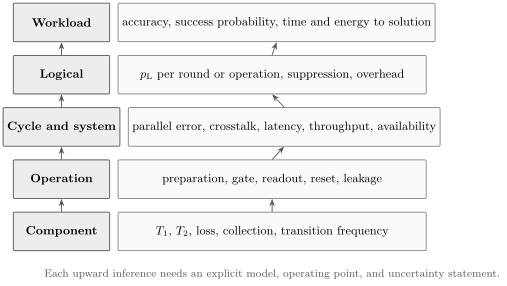
Component quality supports operations; operations compose into simultaneous cycles; cycles support encoded logical behavior; logical operations support workloads. No arrow is automatic. Each upward inference needs operating conditions, a composition model, and uncertainty propagation.

A long $T_1$ does not imply a high-fidelity gate. A high isolated-gate fidelity does not imply low simultaneous-cycle error. A low physical error does not imply logical suppression without a code, syndrome circuit, decoder, and noise model. A low logical error does not imply a useful workload unless rate, scale, compilation, state preparation, readout, and total resource cost are included.

Component Coherence Metrics

Energy relaxation time

For an effective two-level system prepared in $\lvert1\rangle$, an idealized relaxation experiment may fit

$$p_1(t) = B + A e^{-t/T_1}.$$

$T_1$ is the fitted population-relaxation timescale for that transition and operating condition. The offset $B$ can represent thermal population or readout bias; $A$ absorbs imperfect preparation and contrast. A single-exponential fit is a model, not a definition guaranteed by nature. Multiple decay channels, drift, quasiparticle events, atom loss, shelving states, or non-Markovian baths can produce nonexponential curves.

Report at least:

• prepared state and transition;
• idle point, control configuration, and environmental conditions;
• fit function, time range, residuals, and confidence interval;
• repetition schedule and observed drift;
• whether loss is distinguished from relaxation within the computational subspace.

Dephasing times

A Ramsey experiment often fits a signal such as

$$s(t) = B + A e^{-(t/T_2^\ast)^\beta} \cos(\Delta\omega t+\phi).$$

$T_2^\ast$ is an inhomogeneous dephasing time for the Ramsey protocol. The exponent $\beta$ and detuning $\Delta\omega$ encode assumptions about the noise spectrum and control. Hahn echo or longer dynamical-decoupling sequences define different coherence times because they filter low-frequency noise differently. They should not all be labeled simply $T_2$ without the pulse sequence.

For an ideal two-level Markovian model with exponential relaxation and pure dephasing,

$$\frac{1}{T_2} = \frac{1}{2T_1} + \frac{1}{T_\phi}.$$

Within that model, $T_2\le 2T_1$. This relation is a diagnostic model check, not a universal fitting constraint. Dephasing versus Dissipation develops the physical distinction.

Dephasing and Amplitude Damping owns conversion of a protocol-qualified T1–T2 and equilibrium-population record into a finite channel and its physicality, composition, and held-out audits; this page retains metric estimands, acquisition and fit protocols, uncertainty, validity intervals, and reporting boundaries.

Thermal population and state occupancy

An effective qubit may have equilibrium excited-state population

$$p_e^{\mathrm{th}} = \frac{1}{ 1+e^{\hbar\omega/(k_{\mathrm B}T)} }$$

only when a two-level Gibbs model at temperature $T$ is justified. In practice, residual population may arise from nonequilibrium radiation, imperfect reset, leakage, collisions, or detector bias. “Effective temperature” is then a parametrization of one population ratio, not evidence that every device degree of freedom is thermalized at that temperature.

Operation-to-coherence ratio

For operation duration $t_g$,

$$Q_g = \frac{T_2}{t_g}$$

is a useful timescale ratio. It is not a gate count or executable circuit depth. It omits control infidelity, relaxation during other operations, idle periods, routing, leakage, crosstalk, measurement, reset, and error accumulation outside the fitted coherence model.

Preparation, Readout, and Reset

Assignment probabilities

For binary outcomes, write the assignment matrix

$$A = \begin{pmatrix} p(0\mid 0) & p(0\mid 1)\\ p(1\mid 0) & p(1\mid 1) \end{pmatrix}.$$

A commonly reported mean assignment fidelity is

$$F_{\mathrm{assign}} = \frac{ p(0\mid0)+p(1\mid1) }{2}.$$

The two conditional errors should also be reported because the average hides asymmetry. The metric usually includes errors in the reference-state preparations, so it is often a state-preparation-and-measurement quantity rather than a detector-only property.

SPAM Errors owns actual preparation and measurement boundary objects, assignment orientation and license, identifiability and gauge, contextual transfer, and validated correction boundaries. Measurement Error Mitigation owns finite-record correction of a licensed terminal response—stable inverse or forward inference, constraints, calibration covariance, scaling assumptions, residual validation, and overhead; this page retains protocol-qualified hardware estimands, acquisition and fit procedures, uncertainty, validity intervals, and reporting rules.

When loss or leakage is possible, a forced binary classifier can turn a third physical outcome into a misleading bit assignment. Report the confusion matrix over all resolved outcomes, the fraction of rejected or heralded events, and whether rejection is included in the success probability.

Readout fidelity is not one concept

Distinct properties include:

• assignment accuracy: agreement between prepared labels and reported labels;
• quantum non-demolition behavior: whether the postmeasurement state remains in the measured eigenspace;
• measurement efficiency: how much available information is collected relative to measurement-induced disturbance;
• latency: time from the start of readout to a usable classical decision;
• crosstalk: dependence of one result on simultaneous readout of other carriers;
• leakage discrimination: ability to distinguish computational and noncomputational states;
• destructiveness: whether the carrier survives and can be reused.

Repeated agreement of two outcomes is not, by itself, a complete quantum non-demolition metric. Both measurements could be biased, and the first measurement could prepare the state that the second detects.

Initialization and reset

Initialization fidelity should name the target state and whether it is unconditional, heralded, or postselected. Reset needs both a residual-error probability and a duration. A fast active reset with error $\epsilon_{\mathrm{reset}}$ can be more useful than waiting several $T_1$ times, but it may add leakage or correlated disturbance.

For error correction, reset throughput and latency can matter as much as isolated reset fidelity because fresh ancillas must be supplied every syndrome round.

Gate and Channel Metrics

Average gate fidelity

Let $\mathcal E$ be the implemented channel on a $d$-dimensional computational space and $\mathcal U(\rho)=U\rho U^\dagger$ the target. The average gate fidelity is

$$F_{\mathrm{avg}}(\mathcal E,U) = \int d\psi\, \langle\psi\rvert U^\dagger \mathcal E(\lvert\psi\rangle\langle\psi\rvert) U \lvert\psi\rangle.$$

The average gate infidelity is

$$r = 1-F_{\mathrm{avg}}.$$

The integral is over pure input states with Haar measure. Thus $F_{\mathrm{avg}}$ is an average over one use of the channel. It does not describe the worst input, temporal correlation, simultaneous context, or composition over a long circuit.

If $F_e$ is the entanglement fidelity of the error channel $\mathcal U^\dagger\circ\mathcal E$, then

$$F_{\mathrm{avg}} = \frac{dF_e+1}{d+1}.$$

“Process fidelity” is used inconsistently across communities. Some authors mean $F_e$, some mean an overlap of process matrices, and some report a quantity normalized to equal $F_{\mathrm{avg}}$. A paper should give the formula, not only the label.

Worst-case channel distance

A composable worst-case error measure is the diamond distance

$$D_\diamond(\mathcal E,\mathcal U) = \frac{1}{2} \left\| \mathcal E-\mathcal U \right\|_\diamond.$$

The ancillary extension in the diamond norm permits the input to be entangled with another system. This makes the distance suitable for bounding distinguishability and error accumulation, but it is much harder to estimate experimentally than average fidelity.

For a $d$-dimensional channel, general bounds relate infidelity and diamond distance:

$$\frac{d+1}{d}\,r \le D_\diamond \le \sqrt{d(d+1)r}.$$

The wide gap is physically consequential. A small coherent over-rotation can have $r$ quadratic in its angle while $D_\diamond$ is linear. Therefore an average infidelity should not be inserted directly into a worst-case fault-tolerance theorem without a justified noise model or randomization argument. Trace Distance and Fidelity give the reference definitions.

Infidelity is not always an error probability

For a stochastic Pauli channel, infidelity can be proportional to a fault probability. For coherent, nonunital, leakage, or gate-dependent noise, that interpretation can fail. Calling $r$ “the probability the gate failed” silently assumes a stochastic model that the experiment may not establish.

Also declare whether the channel is:

• conditioned on no loss or averaged over loss;
• projected back into the computational subspace;
• corrected for preparation and measurement;
• measured in isolation or during simultaneous operation;
• averaged over a gate set or associated with one target gate.

Characterization and Benchmarking Protocols

No protocol returns “the true fidelity” without assumptions. Each trades information, scalability, and robustness to state-preparation-and-measurement error.

Process tomography

Process Tomography prepares an informationally complete set of inputs and measures an informationally complete set of outputs, or uses an ancilla-assisted equivalent. It can reconstruct a detailed channel model, but its experimental and statistical cost grows rapidly with system size. Ordinary process tomography treats state preparations and measurements as trusted; their errors can be misattributed to the gate.

Tomography is valuable for diagnosing small systems, inspecting coherent structure, and testing models. It is not automatically a scalable system benchmark.

Gate-set tomography

Gate-set tomography jointly estimates preparations, measurements, and a set of gates from long self-consistent circuits. It can reveal coherent and non-Markovian model violations more richly than a single decay parameter. The reconstructed representation has gauge freedom: observable probabilities are unchanged by certain simultaneous transformations of states, measurements, and gates. Gauge-dependent quantities require careful interpretation.

Gate-set tomography is information rich but experimentally and computationally demanding. Its result describes the tested gate-set model and time window, not every circuit context.

Randomized benchmarking

Randomized Benchmarking owns the protocol derivation, sampling design, fit diagnostics, variants, and failure modes. Here the concern is how its reported decay and derived error metric sit beside other hardware metrics.

In reference randomized benchmarking, random gate sequences of length $m$ compose ideally to an inversion. A common fit is

$$P_{\mathrm{surv}}(m) = A p^m+B.$$

$A$ and $B$ absorb state-preparation-and-measurement contrast under the model. For a $d$-dimensional depolarizing channel with decay parameter $p$,

$$r_{\mathrm{RB}} = \frac{d-1}{d}(1-p).$$

This conversion is exact for the declared depolarizing model. Under gate-dependent, context-dependent, or non-Markovian noise, the fitted RB decay still can be stable and useful, but its relationship to an arithmetic mean of individual gate infidelities is subtler. Report the sampled gate group, compilation into native pulses, sequence lengths, number of random sequences, shots, fit model, residuals, and uncertainty.

RB is comparatively insensitive to fixed state-preparation-and-measurement offsets in the decay rate. It is not immune to drift, leakage, sequence-dependent sampling, or model failure, and it does not identify the physical error mechanism.

Interleaved randomized benchmarking

Interleaved RB alternates a target gate with random reference gates. Under standard assumptions, an estimate is

$$r_G \approx \frac{d-1}{d} \left( 1- \frac{p_{\mathrm{int}}}{p_{\mathrm{ref}}} \right),$$

where $p_{\mathrm{ref}}$ and $p_{\mathrm{int}}$ are fitted decay parameters. Gate dependence and interaction between the interleaved gate’s error and the reference errors require bounds or additional analysis. The ratio should not be presented as model free.

Cycle and simultaneous benchmarking

Cycle Benchmarking owns the scheduled-layer protocol, Pauli-orbit decays, dressed-cycle process fidelity, statistical design, and learnability limits.

A cycle is a layer of operations intended to execute in parallel. Cycle benchmarking estimates an error property of the complete implemented cycle, including some simultaneous effects that isolated gate tests miss. Direct randomized benchmarking and related scalable protocols probe larger regions or native gate sets without reconstructing a full process.

These protocols are especially important because a processor executes schedules, not isolated data-sheet gates. A reported cycle metric must state which operations were simultaneous, which qubits were idle, how randomization was implemented, and whether spectator effects were included.

Leakage, Seepage, Loss, and Erasure

Leakage and Crosstalk owns the full-space and survival-branch construction, state and average leakage/seepage/coherence diagnostics, imperfect flags, scalar dynamics, operational crosstalk tests, and context-aware composition; this page retains protocol-qualified metric estimands, acquisition and fit procedures, uncertainty, validity intervals, and reporting boundaries.

Let $P_{\mathrm C}$ and $P_{\mathrm L}$ project onto computational and leakage subspaces of dimensions $d_{\mathrm C}$ and $d_{\mathrm L}$. One average leakage rate for channel $\mathcal E$ is

$$L_1 = \operatorname{Tr} \left[ P_{\mathrm L} \mathcal E \left( \frac{P_{\mathrm C}}{d_{\mathrm C}} \right) \right].$$

An average seepage rate back into the computational subspace is

$$L_2 = \operatorname{Tr} \left[ P_{\mathrm C} \mathcal E \left( \frac{P_{\mathrm L}}{d_{\mathrm L}} \right) \right].$$

In a two-population Markov model, the stationary leakage fraction is

$$p_{\mathrm L}^{(\infty)} = \frac{L_1}{L_1+L_2}.$$

This number depends on the averaging states and model. State-dependent leakage, multiple leakage levels, coherent return, and measurement-induced removal can require a richer description.

Loss means the physical carrier or excitation leaves the accepted system. An erasure is a failure whose location is reliably known to the decoder. Loss becomes an erasure only when it is detected with characterized false-positive and false-negative rates. Postselecting lost trials can improve conditional fidelity while reducing unconditional success; both must be reported.

Crosstalk, Addressability, and Drift

Crosstalk is context dependence: the implemented operation or observation on one subsystem changes when controls, measurements, or states elsewhere change. It can arise from stray fields, shared modes, spectral collisions, classical electronics, detector coupling, heating, or calibration dependencies.

A simple diagnostic compares isolated and simultaneous errors:

$$\Delta r_i = r_i^{(\mathrm{sim})} - r_i^{(\mathrm{iso})}.$$

This difference is useful but not a complete crosstalk model. Crosstalk may create correlated faults even when marginal error rates change little. A serious test varies contexts, checks conditional dependencies, and identifies whether effects are local, pairwise, many-body, static, or time dependent.

Drift means the effective process changes over time. If $\theta(t)$ is a fitted parameter, reporting only

$$\overline\theta = \frac{1}{T} \int_0^T \theta(t)\,dt$$

can hide excursions that invalidate a computation. Include time traces, calibration events, acquisition ordering, and stability intervals. Randomizing the order of experimental settings can reduce confounding between condition and time.

Connectivity, Parallelism, and Scale

Connectivity

Represent directly available two-body interactions by a graph $G=(V,E)$. Useful graph properties include degree, diameter, geometry, edge quality, directionality, and whether edges can be reconfigured. Report the gate or interaction that defines an edge and the operating conditions under which multiple edges are usable simultaneously.

A complete system also needs a conflict graph or scheduling rule. Two edges may each work well in isolation but not at the same time. Connectivity without parallelism can overstate executable depth.

Counts and yield

Distinguish:

• fabricated or available sites;
• occupied carriers;
• detected carriers;
• individually addressable carriers;
• calibrated qubits or modes;
• qubits participating simultaneously in the benchmark;
• data and ancilla qubits in an encoded experiment;
• logical qubits with declared code distance;
• logical qubits supporting the reported operation set.

Calibration yield can be written

$$Y_{\mathrm{cal}} = \frac{N_{\mathrm{meeting\ criteria}}} {N_{\mathrm{tested}}}.$$

The criteria and test duration must be stated. Selecting a high-performing connected subset is legitimate for a benchmark, but the selection rule and fraction of the full device should be visible.

Latency and throughput

For an implemented cycle,

$$\begin{aligned} t_{\mathrm{cycle}} &= t_{\mathrm{prepare}} + t_{\mathrm{control}} + t_{\mathrm{measure}} \\ &\quad + t_{\mathrm{classical}} + t_{\mathrm{feedback}}, \end{aligned}$$

with overlapping intervals treated explicitly. Quantum error correction additionally requires decoder throughput at least equal to the incoming syndrome-data rate and bounded decision latency for adaptive operations.

A shot rate

$$R_{\mathrm{shot}} = \frac{N_{\mathrm{completed\ shots}}}{t_{\mathrm{wall}}}$$

is meaningful only with workload, batch size, reset, compilation, data transfer, and queue boundaries defined. Peak pulse repetition rate is not end-to-end throughput.

Availability may be reported as

$$A_{\mathrm{use}} = \frac{t_{\mathrm{within\ specification}}} {t_{\mathrm{scheduled}}}.$$

The specification should include calibration validity and disabled components. A record obtained during one selected minute and a sustained daily service metric answer different questions.

System-Level Benchmarks

A system benchmark combines width, connectivity, compilation, gates, and readout through a circuit family. It is more representative than one component number but remains task specific.

Cross-entropy benchmarking

Cross-Entropy Benchmarking scores random-circuit samples using ideal probabilities for the same compiled circuits. It probes system-level correlation across gates, concurrency, readout, compilation, and depth, but its interpretation depends on the circuit ensemble, normalization, scrambling regime, noise model, classical reference, and sampling hierarchy.

A linear XEB score is not automatically a state fidelity, distributional distance, or proof of computational advantage. Comparisons require the same circuit family, score convention, postselection policy, probability-computation accuracy, and dated classical baseline.

Quantum volume

Quantum Volume and Application Benchmarks develops the full protocol, statistical unit, volumetric generalization, and application-suite comparison rules. The quantum-volume protocol uses random square model circuits whose width equals their depth. For each width $m$, the compiled device samples outputs, and a heavy-output test determines whether performance exceeds a specified statistical threshold. The reported quantum volume is conventionally

$$V_Q = 2^{m^\star},$$

where $m^\star$ is the largest passing square-circuit size under the protocol.

Quantum volume tests a particular random-circuit family and includes effects of compilation and connectivity. It is not a physical volume, logical-qubit count, general application score, or asymptotic complexity measure. Comparisons require the same protocol version, confidence rule, compiler freedoms, and treatment of selected qubit subsets.

Benchmark families, not universal scores

Other useful system tests include mirror circuits, random circuit sampling, algorithmic benchmark suites, Hamiltonian-simulation tasks, and application-specific validation. No finite suite proves performance on every circuit. A benchmark should expose:

• circuit distribution and instance-selection rule;
• width, depth, native compilation, and optimization budget;
• shots and confidence criteria;
• use of mitigation, postselection, or heralding;
• classical verification cost;
• total wall-clock and classical resources;
• whether the instances were fixed before tuning.

A single-number score is useful for tracking a fixed protocol. It should not erase the underlying performance surface.

Logical Metrics

Logical failure probability

A logical error rate must name its denominator:

$$p_{\mathrm L} = \frac{N_{\mathrm{logical\ failures}}} {N_{\mathrm{logical\ opportunities}}}.$$

An opportunity might be one syndrome round, one unit of memory time, one logical Clifford, one lattice-surgery operation, or one complete circuit. These values are not interchangeable. Also state the code, distance, syndrome schedule, decoder, boundary conditions, leakage handling, and whether detected failures are discarded.

Suppression with code size

For a family of odd-distance codes, a local suppression factor can be defined as

$$\Lambda_d = \frac{p_{\mathrm L}(d)} {p_{\mathrm L}(d+2)}.$$

$\Lambda_d>1$ means the larger tested code performed better under the declared conditions. Sustained below-threshold evidence requires suppression over increasing distances with matched noise, circuits, and decoding. One favorable pair does not prove an asymptotic threshold.

Break-even

An encoded memory reaches break-even only relative to a declared physical baseline. Possible baselines include the best constituent qubit, the average constituent, an unencoded qubit operated for the same wall-clock time, or the best available physical carrier. The baseline should experience comparable preparation, idle time, and measurement opportunities.

Fault tolerance is stronger than break-even. A circuit is fault tolerant when a bounded number of faults cannot spread into an uncorrectable error according to the code and gadget design. Low logical error after postselection is not automatically fault-tolerant correction.

Overhead and logical rate

Report physical qubits or modes, ancillas, spacetime volume, syndrome rounds, decoder resources, distilled resource states, discarded runs, and wall-clock time per logical operation. Logical reliability without rate can hide an architecture that cannot finish the task before drift, memory decay, or practical time limits dominate.

Why Quantum Error Correction Is Possible owns correctability; Surface Code owns distance, repeated syndrome extraction, threshold contracts, and surface-code resource accounting. Logical Benchmarking owns the encoded-memory, gate, scaling, break-even, decoder, and statistical protocols that estimate these logical metrics.

Workload Metrics

The final metric should match the intended task: energy error, sampling distance, decision success, key rate, sensing uncertainty, entanglement-generation rate, or another scientifically meaningful output.

For independent repeated trials with success probability $p_s$ and per-trial time $t_{\mathrm{trial}}$, the number required to reach confidence $C$ of at least one success is

$$N_C = \left\lceil \frac{\ln(1-C)} {\ln(1-p_s)} \right\rceil.$$

The corresponding idealized time to solution is

$$T_{\mathrm{sol}} = N_C\,t_{\mathrm{trial}}.$$

This formula assumes independent stationary trials and a binary success criterion. Verification, queueing, compilation, calibration, and classical postprocessing must be added when they lie inside the operational boundary.

A complete workload resource record can be written schematically as

$$\begin{aligned} \mathcal R = \bigl(& N_{\mathrm{phys}}, N_{\mathrm L}, D, N_{\mathrm{shots}}, t_{\mathrm{wall}}, \\ & E_{\mathrm{total}}, R_{\mathrm{classical}}, \epsilon, C \bigr), \end{aligned}$$

where $D$ is scheduled depth, $\epsilon$ is output error, and $C$ is confidence. Not every study needs every component, but omitted resources should be outside a declared boundary rather than silently ignored.

Uncertainty, Sampling, and Selection

For $k$ observed failures in $N$ independent Bernoulli opportunities,

$$\widehat p = \frac{k}{N}, \qquad \operatorname{SE}(\widehat p) \approx \sqrt{ \frac{\widehat p(1-\widehat p)}{N} }.$$

The normal approximation fails near $p=0$ or $1$ and for small counts. Wilson, likelihood-ratio, Bayesian, or exact intervals are better choices depending on the inferential contract. Observing zero failures does not prove $p=0$; a useful rough $95\%$ upper limit is $3/N$ under independent trials.

Quantum-hardware data often violate independent, identically distributed assumptions:

• drift changes the rate during acquisition;
• calibration is chosen using some of the same data;
• errors are temporally or spatially correlated;
• device subsets are selected after inspection;
• failed preparations or lost carriers are discarded;
• random sequence instances have heterogeneous difficulty.

Use blocked or time-resolved analysis, hierarchical models, held-out validation, and preregistered selection rules where appropriate. At minimum, publish acquisition order, timestamps, calibration interventions, number of discarded runs, and uncertainty method.

Worked Metric Audit

Suppose a report gives the following values for a qubit processor:

Observation	Reported value
Ramsey coherence	$T_2^\ast=100\,\mu\mathrm{s}$
physical gate duration	$t_g=50\,\mathrm{ns}$
qubit RB decay	$p=0.996$
readout conditionals	$p(0\mid0)=0.98$, $p(1\mid1)=0.92$
leakage and seepage	$L_1=2.0\times10^{-4}$, $L_2=2.0\times10^{-2}$
isolated and simultaneous infidelity	$r_{\mathrm{iso}}=0.002$, $r_{\mathrm{sim}}=0.003$
logical failures per round	$p_{\mathrm L}(3)=1.2\times10^{-3}$, $p_{\mathrm L}(5)=5.0\times10^{-4}$

The timescale ratio is

$$\frac{T_2^\ast}{t_g} = \frac{100\,\mu\mathrm{s}}{50\,\mathrm{ns}} = 2000.$$

For qubit RB under the depolarizing conversion,

$$r_{\mathrm{RB}} = \frac{1-p}{2} = 0.002.$$

The mean assignment fidelity is

$$F_{\mathrm{assign}} = \frac{0.98+0.92}{2} = 0.95,$$

but the asymmetric conditionals remain visible. The two-population stationary leakage estimate is

$$\begin{aligned} p_{\mathrm L}^{(\infty)} &= \frac{2.0\times10^{-4}} {2.0\times10^{-4}+2.0\times10^{-2}} \\ &\approx 9.9\times10^{-3}. \end{aligned}$$

Simultaneous operation increases the reported infidelity by

$$\Delta r = 0.003-0.002 = 0.001,$$

or $50\%$ relative to the isolated value. Finally,

$$\Lambda_3 = \frac{1.2\times10^{-3}} {5.0\times10^{-4}} = 2.4.$$

The data show improvement from distance three to five for the tested logical-memory protocol. They do not establish that a depth-2000 circuit succeeds, that all gate errors are stochastic, that the readout is quantum non-demolition, that leakage is state independent, or that suppression continues at larger distance. Each conclusion stays at the layer actually measured.

Reporting Template

A compact hardware-metric record should include:

Metric name and formula:
Layer and physical object:
Target operation or state:
Device subset and connectivity:
Simultaneous context and idle spectators:
Preparation and measurement protocol:
Sequence or circuit distribution:
Fit model and model checks:
Shots, random instances, and acquisition order:
Calibration state and elapsed time:
Point estimate and uncertainty interval:
Leakage, loss, rejection, and postselection:
Compiler, decoder, mitigation, and software versions:
Known blind spots:
Date and raw-data location:

The date belongs in the record because hardware performance and calibration change. The formula belongs there because names such as fidelity, error rate, and throughput are not self-defining.

Common Mistakes

• Reporting fidelity without its object. State, gate, process, assignment, and workload fidelities are different.
• Treating average infidelity as a literal failure probability. This requires a stochastic error model.
• Calling $T_2/t_g$ executable depth. Coherence and control errors do not compose that way.
• Using echo $T_2$ as Ramsey $T_2^\ast$. The pulse sequences filter different noise.
• Hiding asymmetric readout in one average. Report the full assignment matrix.
• Conditioning on survival without reporting loss. Conditional accuracy and unconditional success are both needed.
• Comparing isolated gates with simultaneous cycles. Crosstalk and scheduling change the channel.
• Using an RB number as a worst-case threshold parameter. Average and diamond-distance errors can differ parametrically.
• Calling one improved code distance “below threshold.” Matched suppression over a scaling family is stronger evidence.
• Calling a logical qubit count complete. Code distance, logical operations, error per denominator, and rate must accompany it.
• Publishing a system score without protocol version or compiler conditions. The number cannot be reproduced or compared.
• Quoting zero observed failures as zero error. Finite data imply an upper confidence bound.

Exercises

1. Infer a relaxation time

In an ideal zero-offset model $p_1(t)=e^{-t/T_1}$, the excited-state population is $0.25$ after $30\,\mu\mathrm{s}$. Find $T_1$.

Solution

Taking logarithms,

$$\ln(0.25) = -\frac{30\,\mu\mathrm{s}}{T_1}.$$

Therefore

$$T_1 = -\frac{30\,\mu\mathrm{s}}{\ln(0.25)} \approx 21.6\,\mu\mathrm{s}.$$

A real fit should use all time points and include preparation, thermal offset, uncertainty, and residual checks rather than infer $T_1$ from one point.

2. Combine relaxation and pure dephasing

In the Markovian two-level model, $T_1=100\,\mu\mathrm{s}$ and $T_\phi=80\,\mu\mathrm{s}$. Find $T_2$.

Solution

$$\begin{aligned} \frac{1}{T_2} &= \frac{1}{2T_1} + \frac{1}{T_\phi} \\ &= \frac{1}{200} + \frac{1}{80} \\ &= 0.0175\,\mu\mathrm{s}^{-1}. \end{aligned}$$

Thus

$$T_2 \approx 57.1\,\mu\mathrm{s}.$$

The result is conditional on exponential Markovian relaxation and pure dephasing.

3. Expose readout asymmetry

A detector has $p(0\mid0)=0.995$ and $p(1\mid1)=0.945$. Compute the mean assignment fidelity and both conditional assignment errors.

Solution

$$F_{\mathrm{assign}} = \frac{0.995+0.945}{2} = 0.970.$$

The conditional errors are

$$p(1\mid0) = 0.005, \qquad p(0\mid1) = 0.055.$$

The $97.0\%$ average hides an elevenfold asymmetry between the two errors. That asymmetry can bias observables when state populations are unequal.

4. Convert entanglement fidelity

For a qubit channel, $F_e=0.990$. Find $F_{\mathrm{avg}}$.

Solution

For $d=2$,

$$\begin{aligned} F_{\mathrm{avg}} &= \frac{2F_e+1}{3} \\ &= \frac{2(0.990)+1}{3} \\ &\approx 0.99333. \end{aligned}$$

Thus the average gate infidelity is approximately $6.67\times10^{-3}$. The two fidelity conventions should not be quoted interchangeably.

5. Interpret an RB decay

A qubit randomized-benchmarking fit gives $p=0.994$. Under the depolarizing conversion, find $r_{\mathrm{RB}}$.

Solution

For $d=2$,

$$r_{\mathrm{RB}} = \frac{1-p}{2} = \frac{0.006}{2} = 0.003.$$

This is the RB-derived error parameter under the stated conversion. It is not automatically the diamond distance or the failure probability of every native gate.

6. Compare average and worst-case coherent error

For a small unwanted qubit rotation $e^{-i\theta Z/2}$ relative to the identity,

$$r \approx \frac{\theta^2}{6}, \qquad D_\diamond \approx \frac{\lvert\theta\rvert}{2}.$$

Evaluate both for $\theta=0.02$ radians.

Solution

$$r \approx \frac{(0.02)^2}{6} \approx 6.67\times10^{-5},$$

whereas

$$D_\diamond \approx \frac{0.02}{2} = 0.01.$$

The coherent worst-case distance is about $150$ times the average infidelity. This illustrates why coherent calibration errors can look small under an average metric while remaining important under composition.

7. Find stationary leakage

A two-population model has leakage rate $L_1=3\times10^{-4}$ and seepage rate $L_2=9.7\times10^{-3}$ per cycle. Find the stationary leakage fraction.

Solution

$$\begin{aligned} p_{\mathrm L}^{(\infty)} &= \frac{L_1}{L_1+L_2} \\ &= \frac{3\times10^{-4}} {3\times10^{-4}+9.7\times10^{-3}} \\ &= 0.03. \end{aligned}$$

The model predicts $3\%$ stationary leakage. The result does not describe transient coherent leakage or distinguish several noncomputational levels.

8. Bound an unseen failure rate

No failures are observed in $N=10000$ independent opportunities. Give the rough $95\%$ upper bound from the rule of three.

Solution

$$p_{\mathrm{upper}} \approx \frac{3}{N} = 3\times10^{-4}.$$

The estimate is not zero. Correlation or drift would reduce the effective number of independent opportunities and require a different interval model.

9. Compute logical suppression

Matched experiments give

$$\begin{aligned} p_{\mathrm L}(5) &= 6.0\times10^{-4}, \\ p_{\mathrm L}(7) &= 2.0\times10^{-4}. \end{aligned}$$

Find $\Lambda_5$. If the same factor continued, what would be the projected $p_{\mathrm L}(9)$?

Solution

$$\Lambda_5 = \frac{6.0\times10^{-4}} {2.0\times10^{-4}} = 3.$$

If, and only if, that suppression factor continued,

$$p_{\mathrm L}(9) \approx \frac{2.0\times10^{-4}}{3} \approx 6.7\times10^{-5}.$$

The second result is an extrapolation, not a measurement. Larger codes can encounter new correlations, boundaries, leakage, or decoder bottlenecks.

10. Repair an incomplete metric

A report says, “Our processor has $99.8\%$ fidelity and runs one million operations per second.” List the minimum clarifications needed.

Solution

For fidelity: name the object and formula, target gate or state, device subset, characterization protocol, simultaneous context, treatment of state-preparation-and-measurement error, leakage and loss, fit assumptions, uncertainty, calibration state, and acquisition date.

For rate: define an operation, distinguish physical from logical operations, state the workload and batch size, include preparation, reset, measurement, feedback, compilation, and data transfer, and say whether the number is peak repetition or sustained wall-clock throughput. Without those clarifications the two numbers cannot predict circuit or application performance.

References

1. M. A. Nielsen, “A simple formula for the average gate fidelity of a quantum dynamical operation,” Physics Letters A 303, 249–252 (2002), doi:10.1016/S0375-9601(02)01272-0.
2. A. Gilchrist, N. K. Langford, and M. A. Nielsen, “Distance measures to compare real and ideal quantum processes,” Physical Review A 71, 062310 (2005), doi:10.1103/PhysRevA.71.062310.
3. E. Magesan, J. M. Gambetta, and J. Emerson, “Scalable and robust randomized benchmarking of quantum processes,” Physical Review Letters 106, 180504 (2011), doi:10.1103/PhysRevLett.106.180504.
4. E. Magesan et al., “Efficient measurement of quantum gate error by interleaved randomized benchmarking,” Physical Review Letters 109, 080505 (2012), doi:10.1103/PhysRevLett.109.080505.
5. J. J. Wallman and S. T. Flammia, “Randomized benchmarking with confidence,” New Journal of Physics 16, 103032 (2014), doi:10.1088/1367-2630/16/10/103032.
6. T. Proctor, K. Rudinger, K. Young, M. Sarovar, and R. Blume-Kohout, “What randomized benchmarking actually measures,” Physical Review Letters 119, 130502 (2017), doi:10.1103/PhysRevLett.119.130502.
7. R. Blume-Kohout et al., “Demonstration of qubit operations below a rigorous fault tolerance threshold with gate set tomography,” Nature Communications 8, 14485 (2017), doi:10.1038/ncomms14485.
8. R. Blume-Kohout et al., “Gate set tomography,” Quantum 5, 557 (2021), doi:10.22331/q-2021-10-05-557.
9. A. Erhard et al., “Characterizing large-scale quantum computers via cycle benchmarking,” Nature Communications 10, 5347 (2019), doi:10.1038/s41467-019-13068-7.
10. M. Sarovar, T. Proctor, K. Rudinger, K. Young, E. Nielsen, and R. Blume-Kohout, “Detecting crosstalk errors in quantum information processors,” Quantum 4, 321 (2020), doi:10.22331/q-2020-09-11-321.
11. T. Proctor et al., “Detecting and tracking drift in quantum information processors,” Nature Communications 11, 5396 (2020), doi:10.1038/s41467-020-19074-4.
12. C. J. Wood and J. M. Gambetta, “Quantification and characterization of leakage errors,” Physical Review A 97, 032306 (2018), doi:10.1103/PhysRevA.97.032306.
13. R. Kueng, D. M. Long, A. C. Doherty, and S. T. Flammia, “Comparing experiments to the fault-tolerance threshold,” Physical Review Letters 117, 170502 (2016), doi:10.1103/PhysRevLett.117.170502.
14. A. W. Cross, L. S. Bishop, S. Sheldon, P. D. Nation, and J. M. Gambetta, “Validating quantum computers using randomized model circuits,” Physical Review A 100, 032328 (2019), doi:10.1103/PhysRevA.100.032328.
15. J. Eisert et al., “Quantum certification and benchmarking,” Nature Reviews Physics 2, 382–390 (2020), doi:10.1038/s42254-020-0186-4.
16. Google Quantum AI, “Suppressing quantum errors by scaling a surface code logical qubit,” Nature 614, 676–681 (2023), doi:10.1038/s41586-022-05434-1.
17. D. Bluvstein et al., “Logical quantum processor based on reconfigurable atom arrays,” Nature 626, 58–65 (2024), doi:10.1038/s41586-023-06927-3.
18. M. Kjaergaard et al., “Superconducting qubits: Current state of play,” Annual Review of Condensed Matter Physics 11, 369–395 (2020), doi:10.1146/annurev-conmatphys-031119-050605.
19. National Academies of Sciences, Engineering, and Medicine, Quantum Computing: Progress and Prospects (National Academies Press, 2019), doi:10.17226/25196.
20. P. Krantz et al., “A quantum engineer’s guide to superconducting qubits,” Applied Physics Reviews 6, 021318 (2019), doi:10.1063/1.5089550.

Further Connections

• Threshold Theorem distinguishes theorem parameters, rigorous lower bounds, simulated thresholds, finite-size crossings, and experimental scaling evidence.
• Why Benchmarking Is Hard explains why each metric is a conditional projection, why rankings can reverse across workloads, and how SPAM, context, drift, compiler freedom, verification, and selection constrain a benchmark claim.
• Randomized Benchmarking develops the complete reference and interleaved sequence-decay protocol behind RB metrics, including statistical design and interpretation limits.
• Cycle Benchmarking develops the Pauli-randomized protocol behind dressed process fidelities for fixed scheduled layers and explains orbit, context, and inference limits.
• Cross-Entropy Benchmarking develops random-circuit output scoring, circuit normalization, hierarchical uncertainty, fidelity-model conditions, and classical-verification limits.
• Algorithmic Benchmarking shows how component and system metrics enter task quality, full-stack time, retries, and cost per accepted algorithmic result.
• Process Tomography develops the detailed channel-reconstruction protocol behind tomographic gate metrics and its SPAM, context, uncertainty, and scaling limits.
• Device Characterization explains how spectroscopy, time-domain amplification, GST, randomized diagnostics, and predictive model checks identify mechanisms behind those metrics.
• Reporting Standards specifies how metric definitions, device epochs, sampling hierarchy, exclusions, uncertainty, resources, code, and data travel with a reported value.
• Hardware Overview uses these metrics to compare platform contracts without collapsing them into a winner.
• Control, Readout, and Calibration shows where estimands, uncertainty, held-out tests, latency, crosstalk, and validity intervals enter the operating loop.
• Calibration Loops turns those estimands into monitored validity predicates, candidate-incumbent comparisons, publication gates, and recovery actions.
• Error-Aware Compilation shows how qualified hardware estimands become compiler features and how task-level validation checks the resulting ranking.
• Superconducting Qubits shows how coherence, leakage, assignment, residual coupling, concurrency, and logical metrics enter one physical architecture.
• Quantum Measurement as Estimation develops estimands, likelihoods, estimators, loss, calibration, and uncertainty.
• Claims, Hype, and Evidence Standards separates demonstrations, benchmarks, projections, and application claims.
• Noise in Quantum Information classifies relaxation, dephasing, coherent error, leakage, erasure, correlation, non-Markovianity, and drift.
• Measurement Tomography reconstructs detector effects and explains identifiability assumptions.
• Circuit Model separates ideal, compiled, logical, and physical operations before a rate or fidelity is attached.
• Surface Code supplies the canonical interpretation of distance, syndrome rounds, threshold scaling, and logical resources.
• Logical Benchmarking develops encoded channels, denominators, scaling and break-even comparisons, decoder treatment, and rare-event statistics.
• Resource Estimation carries qualified hardware metrics, code models, and scheduling assumptions into physical-qubit, runtime, failure, and spacetime ledgers.
• Resource Estimation Tools owns scenario execution, uncertainty analysis, validation, and provenance for those estimates.
• Quantum Information Roadmap places metric literacy after circuits, noise, correction, and platform architecture.