Randomized Benchmarking

Short Definition

Randomized benchmarking (RB) estimates an ensemble-average error parameter for implemented quantum gates by measuring how the survival probability of random identity circuits decays with sequence length. In standard reference RB, one samples $m$ gates from a finite group, appends the group inverse, executes the compiled circuit, and asks whether the final state agrees with the intended return state.

Under a baseline model of stationary, Markovian, gate-independent noise and a unitary 2-design such as the Clifford group, the sequence-averaged survival probability is

$$F(m) = A p^m+B.$$

The constants $A$ and $B$ contain fixed state-preparation, measurement, and edge effects. The decay parameter $p$ determines the average infidelity of the twirled noise on a $d$-dimensional computational space:

$$r_{\mathrm{RB}} = 1-F_{\mathrm{avg}} = \frac{d-1}{d}(1-p).$$

This statement is powerful but conditional. RB estimates an average associated with the sampled group, its compiler, its physical context, and its time window. It does not reconstruct a noise channel, identify an error mechanism, return a worst-case error, or automatically yield an error per native gate.

This page is the canonical home for standard reference RB, its twirl derivation, sequence and shot statistics, fit design, interpretation, interleaved RB, and the main failure modes. Metrics for Quantum Hardware owns comparisons among hardware metrics. Process Tomography owns channel reconstruction, while Noise in Quantum Information owns the physical taxonomy of coherent, stochastic, leakage, correlated, and non-Markovian noise. Cycle-level randomized protocols belong to the separate Cycle Benchmarking page.

What Reference RB Estimates

Let $\mathbb G$ be the declared reference group. In a one-qubit experiment it is commonly the 24-element Clifford group; for several qubits, sampled multi-qubit Cliffords must be compiled into available native operations. A reference RB result is attached to the complete implementation map

$$\phi: G\in\mathbb G \longmapsto \text{scheduled pulses, frames, idles, and measurements}.$$

Changing $\phi$ changes the benchmark even when the abstract group is unchanged. Whole-circuit optimization, cancellation, virtual-frame handling, randomized compilation, pulse overlap, spectator activity, and calibration versions are therefore part of the estimand.

The primary object is the mean survival over random sequences:

$$F(m) = \mathbb E_{\boldsymbol G\sim\mathbb G^m} q(m,\boldsymbol G),$$

not the survival of one representative sequence. Here $\boldsymbol G=(G_1,\ldots,G_m)$ and $q$ is the probability generated by the implemented circuit for that particular draw.

Under the standard model, $r_{\mathrm{RB}}$ is an error per sampled reference element. It is often called error per Clifford when $\mathbb G$ is a Clifford group. It is not automatically error per pulse, error per primitive gate, error per layer, or error for the target application.

The Protocol

For each selected length $m$:

1. Draw $G_1,\ldots,G_m$ independently and uniformly from $\mathbb G$.

2. Compute the ideal inverse

   $$G_{m+1} = (G_m\cdots G_2G_1)^{-1}.$$

3. Compile all $m+1$ group elements under a frozen compiler and calibration policy.

4. Prepare a declared state $\rho$, execute the sequence, and measure a declared survival effect $E$.

5. Repeat shots for the same sequence to estimate its survival probability.

6. Repeat with independently sampled sequences at the same $m$.

7. Repeat across lengths and fit the sequence-averaged data.

The implemented sequence channel is

$$\widetilde{\mathcal S}_{\boldsymbol G} = \widetilde{\mathcal G}_{m+1} \circ\widetilde{\mathcal G}_{m} \circ\cdots\circ \widetilde{\mathcal G}_{1},$$

and its survival probability is

$$q(m,\boldsymbol G) = \operatorname{Tr} \!\left[ E\, \widetilde{\mathcal S}_{\boldsymbol G}(\rho) \right].$$

The exact order convention must be fixed in software and tested. An inverse computed with the wrong multiplication order can still produce plausible decay data while benchmarking a different circuit family.

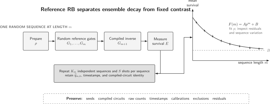
At each length, many random sequences and repeated shots estimate an ensemble mean. The fitted decay $p$ is distinct from the SPAM-dependent contrast $A$ and asymptote $B$; residuals and between-sequence variation remain part of the evidence.

Twirling Under the Baseline Model

Represent an ideal group element by the unitary channel

$$\mathcal G(\rho) = G\rho G^\dagger.$$

Assume each physical implementation has the same Markovian error channel $\Lambda$:

$$\widetilde{\mathcal G} = \Lambda\circ\mathcal G.$$

This gate-independent model is not exact hardware physics; it is the clean starting point from which the standard decay law follows.

The group twirl of $\Lambda$ is

$$\mathcal T_{\mathbb G}(\Lambda) = \frac{1}{|\mathbb G|} \sum_{G\in\mathbb G} \mathcal G^{-1} \circ\Lambda\circ\mathcal G.$$

If $\mathbb G$ is a unitary 2-design and $\Lambda$ is trace preserving, the twirled channel acts as a depolarizing channel on the computational space:

$$\mathcal D_p(\rho) = p\rho +(1-p)\frac{I}{d}.$$

This follows because conjugation leaves the identity direction fixed and acts irreducibly on traceless operators. By Schur’s lemma, a channel commuting with every group conjugation must multiply the entire traceless sector by one scalar $p$.

After averaging independent group draws, the randomized frames convert each interior occurrence of $\Lambda$ into the same twirl. Preparation, measurement, and a final edge channel can be collected into effective objects $\rho'$ and $E'$, giving

$$F(m) = \operatorname{Tr} \!\left[ E'\mathcal D_p^m(\rho') \right].$$

Since

$$\mathcal D_p^m(\rho') = p^m \left( \rho'-\frac{I}{d} \right) +\frac{I}{d},$$

one obtains

$$F(m) = A p^m+B,$$

with

$$\begin{aligned} A &= \operatorname{Tr} \!\left[ E' \left( \rho'-\frac{I}{d} \right) \right], \\ B &= \operatorname{Tr} \!\left( E'\frac{I}{d} \right). \end{aligned}$$

The decay is therefore insensitive to the leading constant SPAM amplitude, not independent of all SPAM behavior.

From Decay to Average Infidelity

The average gate fidelity of a channel $\Lambda$ relative to the identity is

$$F_{\mathrm{avg}}(\Lambda) = \int d\psi\, \langle\psi| \Lambda \!\left( |\psi\rangle\langle\psi| \right) |\psi\rangle.$$

Twirling preserves this average. For $\mathcal D_p$,

$$F_{\mathrm{avg}}(\mathcal D_p) = p+\frac{1-p}{d} = \frac{1+(d-1)p}{d}.$$

Hence

$$r_{\mathrm{RB}} = 1-F_{\mathrm{avg}} = \frac{d-1}{d}(1-p).$$

For a single qubit,

$$r_{\mathrm{RB}} = \frac{1-p}{2}.$$

The conversion is exact for the baseline channel associated with the RB decay. Under gate-dependent noise, modern RB theory can still justify a dominant exponential and an ensemble-level average error under suitable conditions, but the result is not generally the arithmetic mean of separately defined infidelities for every compiled gate.

Worked Example: A Depolarizing Qubit

Suppose the effective one-qubit depolarizing parameter is

$$p=0.998.$$

With ideal preparation and measurement,

$$A=B=\frac12,$$

so

$$F(m) = \frac12(0.998)^m+\frac12.$$

The reported RB infidelity is

$$r_{\mathrm{RB}} = \frac{1-0.998}{2} = 10^{-3}.$$

At length $m=100$,

$$F(100) = \frac12(0.998)^{100}+\frac12 \simeq 0.9093.$$

At $m=500$,

$$F(500) \simeq 0.6838.$$

Long sequences amplify a small per-element decay into observable contrast. They also increase exposure to drift, leakage, heating, and memory. Sequence lengths should span the informative part of the curve rather than merely reach the longest executable circuit.

If SPAM changes the curve to $A=0.42$ and $B=0.47$ while remaining stationary, the same $p$ and $r_{\mathrm{RB}}$ are recovered in the ideal model. The lower contrast increases statistical uncertainty even though it does not change the central decay parameter.

Sequences and Shots Are Different Samples

Let $k=1,\ldots,K_m$ index independently drawn sequences at length $m$, and let $s=1,\ldots,S_{m,k}$ index repeated shots. Conditional on sequence survival $q_{m,k}$,

$$Y_{m,k,s} \sim \operatorname{Bernoulli}(q_{m,k}).$$

The per-sequence estimate is

$$\widehat q_{m,k} = \frac{1}{S_{m,k}} \sum_s Y_{m,k,s},$$

and the unweighted sequence-ensemble mean for equal shot counts is

$$\widehat F(m) = \frac{1}{K_m} \sum_{k=1}^{K_m} \widehat q_{m,k}.$$

Suppose each sequence uses $S$ shots and

$$\sigma_{\mathrm{seq}}^2(m) = \operatorname{Var}_{\boldsymbol G} \!\left[ q(m,\boldsymbol G) \right].$$

The law of total variance gives

$$\operatorname{Var} \!\left[ \widehat F(m) \right] = \frac{\sigma_{\mathrm{seq}}^2(m)}{K_m} + \frac{ \mathbb E_{\boldsymbol G} [q(1-q)] }{K_m S}.$$

The first term is between-sequence variation; the second is shot noise. Once shot noise is small, spending the remaining budget on more shots of the same few sequences does not characterize the random-sequence ensemble. Conversely, one shot on many sequences can be inefficient when readout noise dominates.

Sequence is the experimental unit for the randomization. A bootstrap that resamples only individual shots while holding the sampled circuits fixed omits the first variance term.

Designing Sequence Lengths

Lengths should identify $A$, $p$, and $B$ rather than cluster where the curve is nearly flat. A practical design includes:

• short lengths to resolve initial contrast;
• lengths near the characteristic decay scale;
• long lengths that constrain the asymptote without driving all signal below readout resolution;
• repeated lengths throughout the run to reveal drift;
• more sequence draws where between-sequence variance is large.

For $p$ near one,

$$p^m \simeq \exp[-m(1-p)],$$

so the characteristic scale is approximately

$$m_\star \sim \frac{1}{1-p}.$$

This estimate guides an initial design; a pilot run can then refine the length grid. Selecting lengths after seeing favorable random fluctuations without accounting for that adaptation biases the final analysis.

Fitting the Decay

The familiar three-parameter nonlinear least-squares fit is not the only statistical model. A defensible analysis keeps the data hierarchy visible.

Likelihood and weighting

At minimum, account for heteroskedasticity: survival probabilities near $1/2$ have different binomial variance from probabilities near one, and between-sequence variation can change with $m$. Weighted nonlinear least squares can be useful if weights are estimated honestly. A binomial or hierarchical likelihood retains more of the acquisition model.

Do not first average away sequence identifiers and then treat the resulting point means as equally precise. Preserve counts, sequence seeds, and shots per sequence.

Uncertainty

Useful approaches include:

• hierarchical parametric bootstrap under a declared RB model;
• nonparametric resampling of sequences within each length, with shot resampling nested inside;
• profile-likelihood or Bayesian intervals with transparent priors;
• rigorous concentration bounds when their assumptions and constants fit the experiment.

Report uncertainty in $p$ and propagate it through $r_{\mathrm{RB}}=(d-1)(1-p)/d$. Systematic uncertainty from model failure, compiler variation, drift, or interleaved-RB assumptions is separate from fit uncertainty.

Residuals and alternatives

Inspect residuals against sequence length, acquisition time, random-sequence identity, compiler statistics, and leakage flags. Compare the single exponential with justified alternatives, such as an additional decaying mode for leakage or a transient term for gate dependence. An alternative model is evidence only if it improves predictive behavior on held-out or replicated data, not merely in-sample fit.

What SPAM Robustness Means

Fixed preparation and measurement errors change $A$ and $B$ while leaving the interior decay $p$ unchanged in the baseline derivation. This is the sense in which reference RB is robust to SPAM.

SPAM can still matter in several ways:

• poor preparation or readout reduces $|A|$ and makes $p$ hard to identify;
• reset quality can depend on sequence length or previous outcomes;
• measurement response can depend on leakage or heating accumulated during the sequence;
• the final inversion has sequence-dependent compilation and can correlate edge error with the sampled circuit;
• drift can make $\rho'$, $E'$, $A$, and $B$ vary during acquisition;
• postselection can change the estimand.

Calling RB “SPAM-free” is therefore incorrect. It is insensitive to a particular stationary nuisance structure under a specified model.

Gate-Dependent Noise

Real implementations have

$$\widetilde{\mathcal G} = \Lambda_G\circ\mathcal G,$$

with error depending on $G$, its native decomposition, preceding frames, and simultaneous activity. Gate dependence breaks the elementary replacement of every interior error by one identical twirl.

Perturbative and representation-theoretic analyses show why a dominant exponential often survives. For broad Markovian gate-dependent models, the decay can be written schematically as

$$F(m) = A p^m+B+\Delta(m),$$

where $\Delta(m)$ is a gate-dependent correction that can decay more rapidly than the dominant mode under suitable conditions. This does not license ignoring it. Short-length residuals, strong compilation dependence, or multiple long-lived modes can make a one-exponential summary inadequate.

There is also a gauge issue. Observable circuit probabilities are invariant under simultaneous similarity transformations of state, gates, and measurement. Under gate-dependent noise, relating $p$ to a mean fidelity requires a consistent representation or gauge of the noisy gate set. The RB decay itself is operational; a decomposition into individual gate errors need not be.

Time Dependence and Memory

If the error at step $j$ depends on time or history,

$$\Lambda_j = \Lambda \left( t_j,G_j,G_{<j},h_j \right),$$

then random sequences sample both gates and an evolving environment. Slowly varying Markovian noise may appear as a mixture of nearby exponentials. Quasistatic or correlated noise can produce skewed sequence distributions, nonvanishing variance, shoulders, and acquisition-order dependence.

Defenses include:

• randomizing the order of sequence lengths;
• interleaving reference sequences and calibration checks;
• recording timestamps and control-system state;
• repeating independent epochs rather than pooling them immediately;
• plotting per-sequence and per-epoch distributions;
• testing whether a model fit in one block predicts later blocks.

A visually smooth average decay does not prove Markovianity. Averaging can hide the very correlations that matter to long algorithms.

Markovian and Non-Markovian Noise owns the broader fixed-step, CP-divisibility, causal-break, confounder, and model-escalation tests; this page retains RB sequence design, decay inference, correlated-noise signatures, uncertainty, and benchmark-specific failure modes.

Leakage Breaks the One-Mode Picture

Standard RB assumes a trace-preserving channel on a fixed $d$-dimensional computational space. Leakage violates this closure. Population can leave the space, remain outside it, or seep back, so survival may contain more than one decay mode and need not approach the standard $1/d$ asymptote.

Let $P_{\mathrm C}$ project onto the computational subspace. Measuring both the target-state survival and total computational population,

$$p_{\mathrm C}(m) = \operatorname{Tr} \!\left[ P_{\mathrm C}\rho_m \right],$$

helps separate logical randomization within the subspace from population loss. Leakage RB introduces models for average leakage and seepage rates. Coherent excursions that return during a gate can still generate logical phase error without leaving final population outside the subspace.

Do not force leaky data into $A p^m+B$ and report $r=(d-1)(1-p)/d$ as if the computational channel were trace preserving.

Average Error Is Not Worst-Case Error

Consider a coherent one-qubit overrotation

$$U_\theta = \exp \left( -\frac{i\theta Z}{2} \right).$$

Its average infidelity is

$$r = \frac{1-\cos\theta}{3} \simeq \frac{\theta^2}{6},$$

whereas its diamond distance from the identity is

$$D_\diamond = \left| \sin\frac{\theta}{2} \right| \simeq \frac{|\theta|}{2}.$$

For small $\theta$, average infidelity is quadratic while worst-case error is linear. A stochastic Pauli channel with the same $r$ has very different composition behavior. Standard RB alone does not distinguish these cases.

Unitarity benchmarking modifies the protocol to estimate how strongly a channel preserves the length of traceless operators, providing information about coherent content. It is a complementary statistic, not a conversion of average infidelity into a universal worst-case guarantee.

Error per Clifford Is Not Error per Native Gate

Suppose, only for illustration, that every sampled Clifford consists of exactly $L$ identical native gates with the same depolarizing parameter $p_g$. Then

$$p_{\mathrm C} = p_g^L, \qquad p_g = p_{\mathrm C}^{1/L}.$$

For small errors, dividing an error per Clifford by $L$ approximates the native error. Actual compilations have variable lengths, unequal gate types, virtual operations, cancellation, idle errors, and gate-dependent coherent effects. The observed $p_{\mathrm C}$ is then a weighted circuit property, and naive division need not recover any physical primitive’s fidelity.

At minimum, report the distribution of native gate counts and durations per sampled group element. To characterize one native gate, use a protocol whose theory and randomization directly support that target, such as carefully bounded interleaved RB or an appropriate direct benchmarking protocol.

Interleaved Randomized Benchmarking

Interleaved RB alternates a target gate $G_\star$ with random reference elements. Fit a reference decay $p_{\mathrm{ref}}$ and an interleaved decay $p_{\mathrm{int}}$.

If both reference and target errors act as independent depolarizing channels,

$$p_{\mathrm{int}} = p_{\mathrm{ref}}p_\star.$$

Thus

$$p_\star = \frac{p_{\mathrm{int}}}{p_{\mathrm{ref}}},$$

and the target estimate is

$$r_\star \approx \frac{d-1}{d} \left( 1-\frac{p_{\mathrm{int}}}{p_{\mathrm{ref}}} \right).$$

The approximation sign matters. The target error can interact coherently with reference errors; the interleaved circuit has a different duration and thermal history; and gate-dependent reference errors do not generally factor into one scalar. The original protocol supplies systematic bounds under stated conditions. A ratio with only statistical fit bars should not be presented as model-free gate fidelity.

Reference and interleaved data should be acquired close in time or interwoven so drift does not masquerade as target-gate error.

Other RB Variants

Simultaneous RB

Run reference RB on subsystems separately and then simultaneously. A changed decay is evidence of context or addressability error under the compared schedules. It does not by itself localize the coupling mechanism or predict every parallel workload.

Unitarity RB

Fit a purity-like decay of traceless observables to estimate the unitarity of the noise. Combining unitarity with average infidelity helps distinguish coherent from stochastic behavior, subject to the protocol’s state, measurement, and leakage assumptions.

Leakage RB

Track computational-subspace population as well as target survival and fit a model with leakage and seepage. The measurement must distinguish leaked population, and multiple leakage states or coherent return can require a richer model.

Direct and native-gate RB

Direct RB and related protocols sample customizable native-gate circuits rather than compiling every draw into a large Clifford. They improve scaling and make the sampled operation mix more explicit, but their correctness relies on their own scrambling and error assumptions. “RB” names a family of protocols, not one interchangeable fit.

Character and dihedral protocols

Representation-aware variants isolate selected decay modes or benchmark gate sets smaller than the full Clifford group. Their fitted parameters and conversion formulas must be taken from that protocol’s representation, not copied from standard Clifford RB.

A Defensible Experimental Workflow

1. Declare the estimand. Name the group or gate distribution, subsystem, compiler, native schedule, context, time window, and whether the result is per Clifford, per target gate, or another protocol-specific element.
2. Freeze and validate circuit generation. Test group sampling, composition order, inverse correctness, seed replay, compiler determinism, and native gate accounting.
3. Design lengths and replication. Use a pilot to span the decay, then allocate independent sequences and shots according to both sequence and binomial variance.
4. Randomize acquisition order. Interleave lengths, reference checks, and when relevant interleaved-gate experiments.
5. Preserve raw hierarchy. Store every seed, compiled circuit, native gate count, timestamp, calibration identifier, shot count, outcome, leakage flag, and exclusion.
6. Fit a declared model. State the likelihood or weighting, parameter constraints, initialization, convergence checks, and treatment of overdispersion.
7. Inspect model adequacy. Plot residuals and per-sequence distributions; compare epochs and justified alternative decay models.
8. Propagate statistical uncertainty. Resample sequences, retain nested shot noise, and separate systematic protocol assumptions from fit intervals.
9. Cross-check another protocol. Compare with direct calibration, unitarity, leakage, tomography, simultaneous tests, or workload circuits as appropriate.
10. Publish the evidence bundle. Reproducible Notebooks defines the artifact and clean-execution requirements.

Minimum Reporting Record

Report at least:

• reference group, sampling distribution, subsystem dimension, and target state/effect;
• exact definition of sequence length and whether the inverse is counted;
• sequence lengths, independent sequences per length, shots per sequence, and acquisition order;
• random seeds, generator version, group-composition convention, and inverse tests;
• compiler version, optimization level, native gate counts, durations, virtual operations, idles, and pulse-schedule policy;
• calibration identifiers, timestamps, simultaneous activity, reset policy, leakage treatment, and exclusions;
• raw counts retaining sequence identity;
• fit model, objective or likelihood, weights, parameter constraints, residuals, and alternative-model checks;
• $A$, $B$, $p$, converted $r$, statistical intervals, and any systematic bounds;
• the precise language of the claim: per reference element, per interleaved target, per subsystem, and under which assumptions.

Common Mistakes

Calling RB SPAM-free

RB absorbs stationary leading SPAM factors into $A$ and $B$. Length-dependent reset, leakage-sensitive readout, drift, and poor contrast still matter.

Reporting “gate fidelity” without naming the gate distribution

Reference RB averages over implemented reference elements. The compiler and sampling measure define the average.

Dividing error per Clifford by the mean gate count

This is only a low-error approximation under a restrictive homogeneous model. Variable compilations and gate-dependent errors invalidate the shortcut.

Using one random sequence per length

Repeated shots then estimate that circuit’s survival, not the sequence-ensemble mean.

Bootstrapping shots but not sequences

This omits between-sequence uncertainty and can produce intervals that are far too narrow.

Fitting every curve to one exponential

Leakage, memory, gate-dependent transients, and drift can add modes or overdispersion. The fit form is a hypothesis to test.

Treating interleaved decay ratios as model-free

Reference and target errors need not factor. Report systematic bounds and acquisition timing.

Comparing RB numbers with different compilers

Two experiments over the same abstract Clifford group can implement different native workloads.

Equating average infidelity with worst-case error

Coherent and stochastic channels with the same RB infidelity can compose very differently.

Ignoring chronological order

Pooling an improving or degrading calibration into one curve can produce a precise estimate of no stationary device state.

Further Connections

• Logical Benchmarking lifts randomized sequence tests to encoded gates while retaining syndrome memory, decoder, acceptance, gadget-boundary, and resource caveats.
• Why Benchmarking Is Hard supplies the broader estimand, context, drift, verification, and reporting contract.
• Metrics for Quantum Hardware compares average infidelity with worst-case, leakage, logical, and workload metrics.
• Cycle Benchmarking keeps one scheduled layer fixed, uses local Pauli dressing, and estimates a dressed-cycle process fidelity from Pauli-orbit decays.
• Cross-Entropy Benchmarking scores random-circuit outputs with ideal probabilities, enabling non-Clifford system tests while adding scrambling, classical-reference, and spoofing assumptions absent from reference RB.
• Process Tomography reconstructs a detailed channel model rather than one randomized decay.
• Noise in Quantum Information develops the error mechanisms that can share one RB average.
• Stabilizer Formalism explains Clifford closure, Pauli conjugation, and efficient inverse computation.
• Calibration Loops owns drift detection, acceptance, publication, and rollback of the controls being benchmarked.
• Device Characterization uses RB as one diagnostic coordinate alongside unitarity, GST, mechanism-sensitive amplification, leakage, context, and drift tests.

References

• Joseph Emerson, Robert Alicki, and Karol Życzkowski, “Scalable Noise Estimation with Random Unitary Operators”, Journal of Optics B 7, S347–S352 (2005) — random motion reversal and exponential noise estimation.
• E. Knill et al., “Randomized Benchmarking of Quantum Gates”, Physical Review A 77, 012307 (2008) — early experimental RB protocol and long-sequence gate-error estimate.
• Christoph Dankert, Richard Cleve, Joseph Emerson, and Etera Livine, “Exact and Approximate Unitary 2-Designs and Their Application to Fidelity Estimation”, Physical Review A 80, 012304 (2009) — unitary-design foundation for efficient twirling.
• Easwar Magesan, Jay M. Gambetta, and Joseph Emerson, “Scalable and Robust Randomized Benchmarking of Quantum Processes”, Physical Review Letters 106, 180504 (2011) — standard scalable RB decay and perturbative noise analysis.
• Easwar Magesan, Jay M. Gambetta, and Joseph Emerson, “Characterizing Quantum Gates via Randomized Benchmarking”, Physical Review A 85, 042311 (2012) — detailed derivation, SPAM treatment, and gate-dependence conditions.
• Easwar Magesan et al., “Efficient Measurement of Quantum Gate Error by Interleaved Randomized Benchmarking”, Physical Review Letters 109, 080505 (2012) — target-gate interleaving and systematic bounds.
• Jay M. Gambetta et al., “Characterization of Addressability by Simultaneous Randomized Benchmarking”, Physical Review Letters 109, 240504 (2012) — simultaneous RB for context and addressability.
• Jeffrey M. Epstein, Andrew W. Cross, Easwar Magesan, and Jay M. Gambetta, “Investigating the Limits of Randomized Benchmarking Protocols”, Physical Review A 89, 062321 (2014) — coherent, damping, leakage, and correlated-noise stress tests.
• Joel J. Wallman and Steven T. Flammia, “Randomized Benchmarking with Confidence”, New Journal of Physics 16, 103032 (2014) — sequence variance, experimental design, and confidence bounds.
• Harrison Ball, Thomas M. Stace, Steven T. Flammia, and Michael J. Biercuk, “The Effect of Noise Correlations on Randomized Benchmarking”, Physical Review A 93, 022303 (2016) — sequence distributions under correlated noise.
• Joel J. Wallman, Christopher Granade, Robin Harper, and Steven T. Flammia, “Estimating the Coherence of Noise”, New Journal of Physics 17, 113020 (2015) — unitarity and coherence-sensitive RB.
• Timothy Proctor, Kenneth Rudinger, Kevin Young, Mohan Sarovar, and Robin Blume-Kohout, “What Randomized Benchmarking Actually Measures”, Physical Review Letters 119, 130502 (2017) — operational interpretation and gauge issues under gate dependence.
• Joel J. Wallman, “Randomized Benchmarking with Gate-Dependent Noise”, Quantum 2, 47 (2018) — dominant exponential and decaying correction for general Markovian gate dependence.
• Christopher J. Wood and Jay M. Gambetta, “Quantification and Characterization of Leakage Errors”, Physical Review A 97, 032306 (2018) — leakage, seepage, and leakage RB.
• Robin Harper, Ian Hincks, Chris Ferrie, Steven T. Flammia, and Joel J. Wallman, “Statistical Analysis of Randomized Benchmarking”, Physical Review A 99, 052350 (2019) — resource allocation and principled RB inference.
• Timothy J. Proctor et al., “Direct Randomized Benchmarking for Multiqubit Devices”, Physical Review Letters 123, 030503 (2019) — native-circuit-oriented benchmarking beyond compiled full Cliffords.
• Jonas Helsen, Ingo Roth, Emilio Onorati, Albert H. Werner, and Jens Eisert, “A General Framework for Randomized Benchmarking”, PRX Quantum 3, 020357 (2022) — representation-theoretic multi-exponential framework and fitting analysis.

Exercises

1. Derive the RB decay

Assume the averaged interior noise is $\mathcal D_p$, with effective preparation $\rho'$ and effect $E'$. Derive

$$F(m)=A p^m+B$$

and identify $A$ and $B$.

Solution

Decompose the effective input into identity and traceless parts:

$$\rho' = \left( \rho'-\frac{I}{d} \right) +\frac{I}{d}.$$

The depolarizing channel fixes $I/d$ and multiplies every traceless operator by $p$. Therefore

$$\mathcal D_p^m(\rho') = p^m \left( \rho'-\frac{I}{d} \right) +\frac{I}{d}.$$

Taking the expectation of $E'$ gives

$$\begin{aligned} F(m) &= p^m \operatorname{Tr} \!\left[ E' \left( \rho'-\frac{I}{d} \right) \right] + \operatorname{Tr} \!\left( E'\frac{I}{d} \right) \\ &= A p^m+B. \end{aligned}$$

Thus

$$A = \operatorname{Tr} \!\left[ E' \left( \rho'-\frac{I}{d} \right) \right], \qquad B = \operatorname{Tr} \!\left( E'\frac{I}{d} \right).$$

2. Convert decay to infidelity

An RB fit on a two-qubit computational space returns

$$p=0.9920\pm0.0008.$$

Find $r_{\mathrm{RB}}$ and its propagated one-standard-deviation statistical uncertainty.

Solution

For two qubits, $d=4$, so

$$r_{\mathrm{RB}} = \frac34(1-p) = \frac34(0.0080) = 0.0060.$$

The conversion is linear, hence

$$\sigma_r = \frac34\sigma_p = \frac34(0.0008) = 0.0006.$$

Thus the statistical result is

$$r_{\mathrm{RB}} = 0.0060\pm0.0006.$$

This does not include model, compiler, leakage, or drift uncertainty.

3. Allocate sequences and shots

At one length, suppose the between-sequence variance is $\sigma_{\mathrm{seq}}^2=4\times10^{-4}$ and $\mathbb E[q(1-q)]=0.16$. Compare the variance of the estimated mean for:

1. $K=40$ sequences and $S=100$ shots each;
2. $K=100$ sequences and $S=40$ shots each.

Both designs use $4000$ shots.

Solution

For equal $S$,

$$\operatorname{Var}(\widehat F) = \frac{\sigma_{\mathrm{seq}}^2}{K} + \frac{\mathbb E[q(1-q)]}{KS}.$$

For the first design,

$$\operatorname{Var}_1 = \frac{4\times10^{-4}}{40} + \frac{0.16}{4000} = 10^{-5}+4\times10^{-5} = 5\times10^{-5}.$$

For the second,

$$\operatorname{Var}_2 = \frac{4\times10^{-4}}{100} + \frac{0.16}{4000} = 4\times10^{-6}+4\times10^{-5} = 4.4\times10^{-5}.$$

More sequences reduce the first term, so the second design is better here. The improvement is modest because shot noise dominates. If $\sigma_{\mathrm{seq}}^2$ were larger, the benefit would be greater.

4. Error per compiled element

Assume every one-qubit Clifford contains exactly $L=2$ identical native gates with depolarizing parameter $p_g$, and an RB fit gives $p_{\mathrm C}=0.996$. Find $p_g$ and the corresponding one-qubit native-gate infidelity. State why the calculation is usually only illustrative.

Solution

Under the stated homogeneous model,

$$p_g = \sqrt{p_{\mathrm C}} = \sqrt{0.996} \simeq 0.997998.$$

For a qubit,

$$r_g = \frac{1-p_g}{2} \simeq 1.001\times10^{-3}.$$

Real Clifford compilations have a distribution of native gates, unequal error channels, virtual operations, cancellations, idles, and coherent gate-dependent effects. One scalar $p_{\mathrm C}$ does not generally factor into identical primitive channels.

5. Interleaved RB

A one-qubit reference experiment gives $p_{\mathrm{ref}}=0.9980$, while the interleaved experiment gives $p_{\mathrm{int}}=0.9940$. Compute the depolarizing-ratio estimate of the target-gate infidelity.

Solution

The inferred target depolarizing parameter is

$$p_\star = \frac{0.9940}{0.9980} \simeq 0.995992.$$

For $d=2$,

$$r_\star = \frac12(1-p_\star) \simeq 2.004\times10^{-3}.$$

This is the ratio-model estimate. A complete result also includes statistical propagation, reference gate dependence, target-reference interaction, drift, and the protocol’s systematic bounds.

6. Coherent overrotation

For $\theta=0.02$ radians, estimate the average infidelity and diamond distance of $U_\theta=\exp(-i\theta Z/2)$. Why can one RB number not distinguish this error from a stochastic channel with the same infidelity?

Solution

For small $\theta$,

$$r \simeq \frac{\theta^2}{6} = \frac{(0.02)^2}{6} \simeq 6.67\times10^{-5}.$$

The diamond distance is

$$D_\diamond \simeq \frac{|\theta|}{2} = 0.01.$$

Reference RB primarily estimates the average decay and therefore the average infidelity under its model. Twirling suppresses directional information. A stochastic channel can have the same $r$ but a much smaller worst-case-to- average separation and different composition behavior. A coherence-sensitive protocol such as unitarity benchmarking is needed for more information.

7. Diagnose a drifting experiment

An RB run acquires all short sequences in the morning and all long sequences in the afternoon. Calibration quality degrades monotonically during the day, but the pooled data fit one exponential with small residuals. Is the fitted $p$ a valid stationary gate-set error?

Solution

No. Sequence length is confounded with time. A lower afternoon survival can be explained by length, drift, or both. A smooth exponential does not identify the cause.

The experiment should randomize or interleave lengths, record timestamps and calibration identifiers, repeat reference lengths throughout the run, and compare time blocks. A hierarchical model may estimate time dependence, but it cannot recover information absent from the confounded acquisition. The pooled $p$ can be reported only as a property of that chronological campaign, not a stationary gate set.

8. Detect leakage-model failure

Suppose target-state survival decays below $1/d$ and total computational-space population also decreases with length. Explain why the standard RB conversion is invalid and name the additional observables needed for a leakage analysis.

Solution

The standard derivation assumes a trace-preserving channel on the $d$-dimensional computational subspace. Decreasing computational population violates that assumption, and the asymptote and decay modes need not match $A p^m+B$. The fitted $p$ cannot be converted to

$$r=\frac{d-1}{d}(1-p)$$

as though it described a closed depolarizing channel.

A leakage analysis should separately estimate target-state survival and total computational-subspace population. If the detector resolves leakage levels, their populations are also useful. A model with leakage and seepage rates, and possibly multiple or coherent leakage modes, should be fitted and validated.