Why Benchmarking Is Hard

Short Definition

A quantum-computer benchmark is a specified experiment that maps a device, software stack, operating condition, and workload ensemble to measured performance with an uncertainty statement. It does not reveal an intrinsic scalar called “quantum-computer power.”

A complete benchmark can be represented schematically by

$$B = \left( \mathcal T,\mu,\Pi,\mathcal I,\mathcal S,\mathcal A \right),$$

where $\mathcal T$ is the task family, $\mu$ the instance distribution, $\Pi$ the execution protocol, $\mathcal I$ the allowed implementation policy, $\mathcal S$ the scoring and pass rule, and $\mathcal A$ the statistical analysis. The reported value is conditional on all six, on the device state at the time of execution, and on software and data versions.

This page owns the conceptual reason benchmarking is difficult: capability is multidimensional, noise is contextual and time dependent, measurements are imperfect, useful outputs can be hard to verify, and implementation choices can change what was actually tested. Metrics for Quantum Hardware owns operational definitions and formulas for component, gate, cycle, system, logical, and workload metrics. Future pages in this chapter own individual tomography, randomized-benchmarking, cross-entropy, application-benchmark, and advantage-verification protocols. Claims, Hype, and Evidence Standards owns the labels attached to the resulting claims.

Capability Is a Conditional Surface

For a fixed processor, success depends on more than qubit count or one average error rate. Let $C$ denote a circuit or task instance and let $\lambda$ collect execution choices. A useful abstract object is

$$q = q(C,\lambda,t),$$

where $q$ is an output-quality measure and $t$ labels the device and calibration state. The execution choices can include qubit subset, mapping, routing, scheduling, native synthesis, pulse realization, mitigation, postselection, decoder, shot count, and classical optimizer.

A benchmark samples only part of this surface. For width $w$ and depth $d$, for example, it may estimate

$$\overline q_B(w,d) = \mathbb E_{ C\sim\mu_B(w,d) } \left[ q(C,\lambda_B,t) \right].$$

The subscript $B$ matters. A different circuit ensemble, compiler policy, score, or time window defines a different average. Even if both studies use the word “fidelity,” they need not estimate the same object.

This immediately explains why one number is not universal. Suppose devices $A$ and $B$ satisfy

$$\begin{aligned} q_A(C_1)&>q_B(C_1),\\ q_A(C_2)&<q_B(C_2). \end{aligned}$$

Neither device is globally better. A task distribution concentrated near $C_1$ ranks $A$ first; one concentrated near $C_2$ ranks $B$ first. Crossing performance curves are normal when devices differ in connectivity, native gates, measurement, speed, crosstalk, or logical support.

A Benchmark Is a Projection

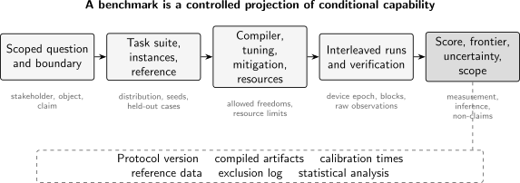
Every benchmark projects conditional device behavior onto a report. The task ensemble, implementation freedom, device epoch, reference answer, score, and statistical rule are part of the result rather than incidental laboratory details.

The projection can be useful. A scalar is easy to track over time, use as a release gate, or compare under a fixed protocol. The danger begins when its scope is forgotten.

If a benchmark compresses $K$ normalized metrics into

$$S_{\mathbf w} = \sum_{k=1}^{K} w_k m_k, \qquad w_k\geq0, \qquad \sum_k w_k=1,$$

then the weights $\mathbf w$ encode priorities. One stakeholder may emphasize accuracy, another time to solution, another logical reliability, and another availability or energy. Different defensible weights can reverse the ranking. The score is therefore a decision model, not a discovery that the device has one natural position on a universal scale.

Whenever practical, publish the underlying performance surface or Pareto frontier as well as any scalar summary. A reader can then see whether a score rose because the device improved broadly, because one operating point improved, or because the benchmark policy changed.

What Exactly Is Being Benchmarked?

Several layers are routinely called “the performance of the computer.”

Layer	Typical question	Useful output	Important blind spot
component	How stable is one physical degree of freedom?	$T_1$, $T_2$, loss, temperature, contrast	control, simultaneous operation, software
preparation and measurement	How accurately are states initialized and outcomes assigned?	confusion matrix, reset error, detection loss	gate and memory errors
gate or cycle	How well is a declared operation or simultaneous layer implemented?	fidelity, decay, unitarity, leakage, cycle error	arbitrary workload behavior
system or volumetric	Which circuit shapes and structures pass a fixed quality rule?	width–depth map, frontier, aggregate score	application representativeness
logical	How reliably and quickly does encoded information behave?	logical failure per round or operation, suppression, rate	full algorithm cost
application	Does a named task achieve its output criterion?	answer error, success probability, time to solution	transfer to other tasks
service	What can a user complete under operational constraints?	throughput, latency, availability, cost, reproducibility	internal diagnostic detail

These layers are complementary. A component benchmark can diagnose a material or control bottleneck. A gate benchmark can guide calibration. A volumetric benchmark can map a broad circuit capability. An application benchmark can answer a user-facing question. A logical benchmark can establish error suppression. Asking one layer to answer all the others creates misleading comparisons.

The benchmark boundary also matters. Does “runtime” begin before compilation, after queue admission, at the first pulse, or at the first accepted shot? Does it include reset, calibration, decoding, mitigation, classical optimization, network transfer, verification, and retries? Each boundary is legitimate for some question, but the boundaries are not interchangeable.

Four Different Activities

Benchmarking is often mixed with three neighboring activities:

Activity	Central question	Typical result
characterization	What model or parameters describe the implementation?	reconstructed state, channel, detector, or noise parameters
verification	Does an implementation meet a specified target or acceptance rule?	pass decision, witness, distance, or fidelity bound
validation	Does the model or system predict behavior relevant to its intended use?	held-out agreement across regimes or tasks
benchmarking	How does performance score under a standardized workload and protocol?	metric, curve, frontier, or ranked report

A benchmark may use characterization data and a verification test, but the words should not be treated as synonyms. Reconstructing a one-qubit channel does not validate a many-qubit application. Passing a random-circuit score does not characterize the noise mechanism. Matching a fitted noise model on training circuits does not show that it predicts held-out workloads.

Exponential State Space Limits Direct Inspection

An arbitrary mixed state of $n$ qubits requires

$$4^n-1$$

real parameters. A general process is larger still. Full tomography therefore cannot be the routine acceptance test for a large processor, even before accounting for the circuits and samples needed to identify those parameters accurately.

Scalable protocols avoid full reconstruction by estimating selected properties: average decays, local observables, cycle fidelities, output scores, conserved quantities, or success on structured circuits. This is a strength, but it creates a scope condition. A protocol that efficiently estimates one projection cannot certify every unmeasured error direction.

There is a recurring practical tension among:

• scalability: the protocol remains feasible as width and depth grow;
• informativeness: the result diagnoses the errors relevant to a decision;
• representativeness: the workloads resemble intended applications;
• verifiability: a trustworthy reference or acceptance test is available.

No theorem says only one can be achieved, but demanding all four at once is usually difficult. Exact small circuits are verifiable but may be too easy. Large random circuits stress the processor but can be expensive to verify. Application circuits are representative only for a particular use and may mix hardware, compiler, optimizer, and input-model effects.

SPAM and the Trusted-Reference Problem

Experiments do not observe a gate directly. With prepared state $\rho$, implemented circuit $\widetilde{\mathcal C}$, and measurement effect $M_x$, the observed probability is

$$p_{\mathrm{obs}}(x|C) = \operatorname{Tr} \left[ M_x\, \widetilde{\mathcal C}(\rho) \right].$$

An unexpected probability can arise from state preparation, the circuit, measurement, or their correlations. If preparation and measurement are assumed perfect, their errors may be incorrectly assigned to the gate. If all three are estimated self-consistently, gauge freedoms and model adequacy must be handled.

Randomized benchmarking was designed in part to make an average decay insensitive to leading state-preparation-and-measurement amplitudes under its model. That does not make SPAM nonexistent, identify every gate error, or guarantee workload accuracy. Tomography is more descriptive but has scaling, gauge, and model-selection costs. State Tomography develops reconstruction under a trusted measurement model, while Process Tomography extends that inverse problem to channels. Randomized Benchmarking develops the distinct sequence-decay contract, including its twirl assumptions, sampling hierarchy, fit diagnostics, and interpretation limits.

The general lesson is not to seek a protocol with no assumptions. It is to state which operations are trusted, which are estimated jointly, and which failure modes remain invisible.

Context Makes Local Numbers Noncompositional

A physical operation is rarely one fixed channel independent of use. A more honest model is

$$\widetilde{\mathcal G}_k = \widetilde{\mathcal G}_k \left( t,q_k,C_{<k},C_{\parallel k},h_k \right),$$

where $q_k$ is placement, $C_{<k}$ the preceding history, $C_{\parallel k}$ simultaneous activity, and $h_k$ hidden classical or environmental state. Frequency collisions, spectator shifts, leakage, heating, controller memory, measurement backaction, and decoder latency can all introduce context dependence.

Consequently, multiplying isolated-gate fidelities is generally not a validated circuit model. Even stationary local errors can compose differently according to their coherence.

For a coherent overrotation

$$U_\epsilon = e^{-i\epsilon Z/2},$$

the average infidelity from the identity is

$$r_1 = \frac{1-\cos\epsilon}{3} \approx \frac{\epsilon^2}{6}.$$

After $L$ identical coherent repetitions,

$$r_L = \frac{1-\cos(L\epsilon)}{3} \approx \frac{L^2\epsilon^2}{6}$$

while small independent stochastic errors often accumulate approximately linearly for short sequences. Two devices with the same single-gate average infidelity can therefore have very different deep-circuit behavior.

Cycle Benchmarking and simultaneous benchmarks probe some context that isolated tests miss. Application and mirror circuits probe other structures. None samples every possible history or concurrency pattern, so a benchmark suite should vary the contexts relevant to the intended workload.

Non-Markovian Noise and Drift

Many benchmark analyses use stationary or Markovian models because they make estimation possible. Real devices can drift during the experiment, retain memory across controls, or switch between latent operating modes.

If a parameter $\theta(t)$ changes during data collection, the reported value is effectively a schedule-dependent average,

$$\overline\theta = \int w(t)\theta(t)\,dt, \qquad \int w(t)\,dt=1.$$

Running all short circuits first and all long circuits later can turn drift into an apparent depth dependence. Running device $A$ in the morning and device $B$ in the evening can turn laboratory time into a platform difference. Calibrating on the same instances later reported as the benchmark can hide generalization failure.

Useful controls include:

• randomizing or interleaving circuit order;
• repeating reference circuits throughout the run;
• recording calibration epochs and control revisions;
• blocking the analysis by time and checking stationarity;
• reserving held-out instances;
• reporting between-day and within-day variation;
• preserving failed or interrupted blocks with explicit exclusion reasons.

Calibration Loops owns the lifecycle of calibration records, drift triggers, acceptance, and rollback. A benchmark should consume that provenance rather than treating a device name as a stationary experimental condition.

Compiler Freedom Can Change the Test

A logical benchmark circuit is not automatically the circuit that reaches the hardware. Mapping, routing, gate synthesis, optimization, scheduling, pulse selection, dynamical decoupling, mitigation, and postselection can all change the physical workload.

Implementation freedom is neither always good nor always bad:

• unrestricted optimization measures the best available system stack;
• fixed compilation isolates hardware more directly;
• a fixed native circuit improves comparability but may disadvantage a platform whose natural operations differ;
• platform-specific optimization can answer an end-user question while obscuring which layer caused the difference.

The policy must be part of the benchmark. Record the source circuit, compiled artifact, native gate counts, scheduled depth, qubit map, compiler version, optimization budget, human tuning, pulse or target revision, mitigation, and discarded shots.

A compiler that recognizes and deletes most of a nominally difficult circuit may be demonstrating excellent software. It may also mean the benchmark no longer stresses the intended hardware capability. The correct interpretation depends on whether compilation was inside the declared system boundary.

Accuracy, Speed, and Resources Trade Off

Output quality is only one dimension. Consider a performance vector

$$\mathbf m = \left( q, t_{\mathrm{wall}}, N_{\mathrm{shot}}, R_{\mathrm{classical}}, E, A \right),$$

where $q$ is quality, $R_{\mathrm{classical}}$ classical resources, $E$ energy, and $A$ availability. Error mitigation may improve $q$ while increasing shots and wall time. Postselection may improve conditional accuracy while reducing acceptance probability. Slower gates may improve fidelity but reduce throughput. Larger codes may suppress logical errors while increasing space and latency.

Report both conditional quality and acceptance:

$$p_{\mathrm{useful}} = p_{\mathrm{accept}}\, p_{\mathrm{correct}\mid\mathrm{accept}}.$$

Reporting only the second factor can make aggressive postselection look like unconditional performance. Likewise, “quantum execution time” and end-to-end time to solution answer different questions. Queueing may be outside a hardware study but inside a service study; compilation and verification may be outside a pulse experiment but inside an application workflow.

When no device dominates all relevant dimensions, publish a Pareto comparison instead of forcing an arbitrary winner.

Statistical Uncertainty Is Only One Uncertainty

For $k$ successes in $N$ independent Bernoulli trials,

$$\widehat p = \frac{k}{N}.$$

Finite-shot uncertainty can be quantified with a stated interval. But more shots reduce only sampling uncertainty under the assumed process. They do not remove model error, drift, selection bias, reference error, compiler dependence, correlated samples, or an unrepresentative task ensemble.

Benchmark reports should separate at least:

• finite-shot or finite-sequence uncertainty;
• variation across circuit instances;
• variation across time blocks and calibrations;
• uncertainty in the reference answer;
• fit and model-selection uncertainty;
• sensitivity to compiler and analysis choices;
• systematic omissions that are not probabilistically quantified.

Selection must also be counted. If $K$ independent configurations are tested at a per-test false-positive rate $\alpha$ and only the best is reported, the chance of at least one false positive is

$$p_{\mathrm{any}} = 1-(1-\alpha)^K.$$

The independence assumption is often imperfect, but the formula shows the direction of the bias. Predeclare the selection rule, disclose the search space, use held-out confirmation, and report whether qubits, compiler seeds, mitigation settings, fit windows, or stopping times were chosen after looking at results.

Verification Gets Hard Near the Interesting Regime

A benchmark needs a reference: an exact answer, a distributional property, an efficiently checkable witness, a conserved quantity, or an acceptance protocol. For small generic circuits, exact classical simulation can supply the answer. As width and entanglement grow, the reference calculation can become the dominant cost.

This creates the verification gap: the regimes most interesting for demonstrating quantum computational capability can be the regimes where a classical verifier cannot calculate every ideal probability.

Useful strategies include:

• exact comparison on smaller instances and controlled scaling;
• analytically solvable limits and conserved quantities;
• circuits with efficiently computable ideal outputs;
• mirror or Loschmidt-style constructions with a known target;
• local observable, symmetry, or stabilizer checks;
• cross-validation among independent classical methods;
• hidden challenge instances and blind analysis;
• interactive or cryptographic verification protocols when their assumptions and overhead fit the claim;
• independent reproduction on another implementation.

Each strategy verifies something different. A mirror circuit can have a known ideal output while failing to represent an application. Local observables can agree while a global state is wrong. Small-instance agreement supports an extrapolation only when the scaling model is tested. Complexity-theoretic hardness does not by itself prove that an experimental sample came from the target distribution.

Quantum Circuit Simulation owns exact and structure-aware simulation contracts. Verification of Quantum Advantage owns the full correctness, hardness, classical-frontier, adversarial, and reproduction logic for claims beyond straightforward classical verification.

Classical Baselines Are Moving Experimental Objects

An application or advantage comparison requires a classical baseline. “A supercomputer” is not a baseline specification. Record:

• the exact task, input distribution, output tolerance, and confidence;
• the classical algorithm and approximation;
• implementation, compiler, numerical libraries, and precision;
• processor, accelerator, memory, interconnect, and parallelism;
• preprocessing, data loading, checkpointing, and output verification;
• wall-clock, energy, monetary, and human-tuning boundaries;
• code and parameter availability;
• the date and known alternative algorithms.

The fastest known classical method can improve after a quantum experiment is published. That does not erase the historical experiment, but it changes a claim of continuing advantage. Report a comparison against named implementations and hardware at a date, and separate it from an asymptotic complexity statement.

Fairness does not always mean identical hardware resources. It means the comparison answers a declared decision. A scientific question may compare best-known methods at equal output error. A service question may compare end-to-end wall time and cost. An energy study must include the relevant control and classical systems on both sides.

Designing a Defensible Benchmark

Noise, Channels, and Error Mitigation supplies the mechanism, model, context, intervention, and accepted-answer cost ledger; this page retains benchmark estimands, experimental design, uncertainty, comparability, classical baselines, and evidence limits.

Start with the decision

Identify who will use the result and what choice it informs. Calibration engineers, architecture researchers, algorithm developers, procurement teams, and end users need different benchmarks.

Write the claim before choosing the score:

Under a frozen task distribution, implementation policy, operating window, and uncertainty rule, this system reaches the declared quality threshold over this region of problem size or circuit shape.

That claim is narrower than “device $A$ is the best quantum computer,” and much more useful.

Freeze the contract

A minimum benchmark contract records:

Field	Required content
object	device, subsystem, gate set, logical layer, software stack, or service
task family	circuits or instances and their scientific meaning
sampling	fixed suite or generator, distribution, seeds, and held-out split
implementation	allowed compilation, mapping, tuning, mitigation, and postselection
operating state	hardware subset, calibration, firmware, software, timing, and concurrency
reference	exact, analytic, simulated, witnessed, or otherwise verified target
score	formula, normalization, aggregation, and direction of improvement
acceptance	threshold, confidence, multiple-testing, and stopping rule
resources	shots, wall time, classical compute, energy, cost, and excluded resources
provenance	raw data, artifacts, versions, timestamps, exclusions, and review status

Version the contract. A score produced under version two should not be placed on the same trend line as version one without a bridge study.

Sample a region, not one showcase

Use a fixed ensemble or a public generator with declared randomness. Vary width, depth, structure, placement, concurrency, and application parameters that matter. Include edge cases and intentionally hostile instances where scientifically appropriate.

For a volumetric benchmark, define a success region such as

$$\mathcal R_B(\tau) = \left\{ (w,d): \overline q_B(w,d)\geq\tau \right\}.$$

The boundary of $\mathcal R_B$ carries more information than the largest passing square alone. A device optimized for narrow deep circuits and one optimized for wide shallow circuits can have similar scalar scores but different frontiers.

Separate tuning from evaluation

Use training instances for calibration, compiler tuning, and mitigation selection. Use held-out instances and, where possible, a later time block for the reported evaluation. If the same data serve both roles, state that the result is in-sample.

Publish the evidence bundle

Release source and compiled circuits, instance generators, seeds, raw counts, calibration records, analysis code, environment, reference data, uncertainty calculation, exclusion log, and summary tables when permissions allow. Reproducible Notebooks gives the corresponding executable-artifact contract. A screenshot of a leaderboard is not a reproducibility package.

Comparing Results Without Overclaiming

There are several levels of comparability:

1. Longitudinal: the same system under the same protocol at different times.
2. Cross-system, same contract: different systems under the same task, implementation freedoms, reference, score, and analysis.
3. Cross-platform, adapted contract: semantically equivalent tasks with platform-specific compilation and explicit normalization.
4. Cross-paradigm: gate-model, annealing, analog, photonic, or continuous-variable systems compared only at a common application output and resource boundary.

Comparability weakens down the list. A platform-neutral source language does not guarantee equal physical workloads, while forcing identical native gates can be physically meaningless. For cross-paradigm studies, begin at the problem and success criterion rather than pretending the internal operation counts are the same.

A useful report distinguishes:

• measurement: what the protocol directly observed;
• inference: what follows under stated assumptions;
• extrapolation: what a fitted model predicts outside the tested region;
• comparison: what is established relative to named alternatives;
• non-claim: what the benchmark was not designed to show.

Worked Benchmark Audit

Suppose a report says:

Processor $A$ has twice the benchmark score of processor $B$, so it is twice as useful.

The conclusion does not follow. An audit asks:

1. What task ensemble and protocol define the score?
2. Is the scale linear, logarithmic, or a threshold label?
3. Were the same confidence and pass rules used?
4. Were qubit subsets selected after testing?
5. What compilation and mitigation were allowed?
6. Do accepted-shot and unconditional costs differ?
7. Were the devices measured in interleaved time blocks?
8. Does the intended application resemble the benchmark circuits?
9. Do quality, runtime, availability, and classical overhead tell the same story?
10. Can the reference calculation and raw data be audited?

For example, a score of the form $2^{m^\star}$ changes by a factor of two when the largest passing integer $m^\star$ increases by one. That does not mean every application becomes twice as accurate or twice as fast. It means one additional size passed a specific threshold under that protocol. Metrics for Quantum Hardware owns the quantum-volume definition and its operational qualifications.

The repaired conclusion is:

Under benchmark version $v$, processor $A$ passed size $m_A^\star$ and processor $B$ passed $m_B^\star$, with the reported confidence, compiler policy, selected subsets, and execution dates. This compares performance on the benchmark’s random square-circuit family; application relevance requires separate evidence.

Common Mistakes

• Ranking devices by qubit count without quality, connectivity, speed, or logical behavior.
• Treating an average gate error as an independent stochastic failure probability.
• Multiplying isolated component metrics to predict a contextual workload.
• Calling a SPAM-robust fit SPAM-free.
• Hiding drift by pooling all shots into one interval.
• Comparing devices measured at different times without interleaving or qualification.
• Allowing different compiler, mitigation, or postselection budgets without reporting them.
• Reporting conditional accuracy without acceptance probability.
• Choosing the best qubit subset, seed, fit window, or stopping time after inspecting the data.
• Treating one random-circuit, application, or logical benchmark as universal.
• Using classically tractable instances without testing transfer to the claimed regime.
• Using intractability as proof of correctness.
• Comparing against an unnamed or obsolete classical baseline.
• Changing a benchmark specification without versioning the score.
• Publishing a scalar without the performance surface, uncertainty, raw data, and scope statement.

Exercises

1. Show that ranking depends on the task

Device $A$ succeeds with probabilities $0.99$ and $0.60$ on task families $C_1$ and $C_2$. Device $B$ succeeds with probabilities $0.94$ and $0.85$. For a benchmark that samples $C_1$ with probability $w$, when does $A$ rank above $B$?

Solution

The average scores are

$$\begin{aligned} S_A &= 0.99w+0.60(1-w), \\ S_B &= 0.94w+0.85(1-w). \end{aligned}$$

Their difference is $S_A-S_B=0.30w-0.25$. Therefore $A$ ranks above $B$ only when

$$w>\frac{5}{6}.$$

Neither device has a task-independent ranking. The benchmark’s instance distribution decides which tradeoff matters.

2. Compare coherent and stochastic accumulation

A coherent $Z$ overrotation has $\epsilon=10^{-2}$ radians. Estimate the single-gate average infidelity and the small-angle infidelity after $L=100$ identical repetitions. Why is multiplying the single-gate value by $100$ misleading?

Solution

For one gate,

$$r_1 \approx \frac{\epsilon^2}{6} = 1.67\times10^{-5}.$$

For one hundred coherent repetitions, $L\epsilon=1$, so the exact expression is

$$r_{100} = \frac{1-\cos 1}{3} \approx 0.153.$$

The small-angle quadratic estimate gives $100^2\epsilon^2/6\approx0.167$, which is already only approximate at angle one. Multiplying $r_1$ by $100$ would give about $1.67\times10^{-3}$ and miss coherent buildup by two orders of magnitude.

3. Separate sampling from drift

A benchmark collects $10^6$ shots over twelve hours and reports a tiny binomial standard error. Reference-circuit success drifts from $0.98$ to $0.90$ during the run. Is the pooled interval an adequate uncertainty statement?

Solution

No. The binomial interval conditions on a stationary independent success probability. The observed drift violates that model and can bias comparisons if circuit families were run in different time blocks. Report time-resolved results, randomize or interleave circuit order, model or bound between-block variation, and state the operating window. More shots do not remove nonstationarity.

4. Audit postselection

A mitigation procedure accepts $4\%$ of shots and reaches conditional correctness $0.995$. What is the unconditional probability of obtaining an accepted correct result in one raw shot?

Solution

It is

$$p_{\mathrm{useful}} = 0.04\times0.995 = 0.0398.$$

The benchmark should report both the conditional correctness and the acceptance rate. A time-to-solution calculation must include the rejected shots and any mitigation overhead.

5. Quantify selection risk

Twenty independent qubit subsets are tested with a nominal per-subset false-positive rate $\alpha=0.05$, and only the best subset is reported. Under the independence model, what is the chance of at least one false positive?

Solution

The probability is

$$1-(1-0.05)^{20} \approx 0.642.$$

The subsets may not be independent in practice, but the calculation shows why an undisclosed search invalidates the nominal 5% interpretation. Predeclare the subset or confirm the selected subset on held-out data with an adjusted analysis.

6. Repair a compiler comparison

Two platforms receive the same logical circuit. Platform $A$ uses unrestricted optimization; platform $B$ uses optimization disabled. Platform $A$ wins. What can and cannot be concluded?

Solution

The result may compare two complete workflows under unequal implementation policies, but it does not isolate hardware capability and is not a fair same-contract system comparison. Re-run with a shared optimization policy or declare that each platform receives the same optimization budget and may use its best stack. Preserve source and compiled circuits, native counts, schedules, versions, and tuning effort. The first design benchmarks hardware more directly; the second benchmarks end-to-end stacks.

7. Choose a verification strategy

A circuit family becomes too large for exact state-vector verification but has a conserved parity and admits smaller exact instances. Give a defensible validation ladder.

Solution

Verify exact output distributions on smaller widths and depths; test parity on every size; compare two independent classical methods in their overlap; include mirror or known-answer circuits with similar width, depth, and native structure; test scaling of errors rather than extrapolating one point; and reserve hidden instances. State that these checks do not reconstruct the large-instance distribution. Independent implementation or an interactive verification protocol would strengthen a larger claim.

8. Decide whether one device dominates

For the same application accuracy, device $A$ takes $10$ s and $10^5$ raw shots; device $B$ takes $25$ s and $2\times10^4$ shots. All other declared resources are equal. Which device is better?

Solution

Neither dominates: $A$ has lower wall time, while $B$ uses fewer shots. A ranking requires an external cost model, throughput constraint, energy model, or service objective. Report both as Pareto points rather than hiding the tradeoff in an unexplained scalar.

Research Status

The need for explicit benchmark contracts, uncertainty, task ensembles, implementation policies, and scope statements is established. Randomized, tomographic, cycle, mirror, volumetric, logical, and application-oriented protocols provide complementary views of quantum systems.

The benchmark landscape remains active. Researchers continue to improve scalable verification, context sensitivity, logical benchmarks, application suites, time-to-solution accounting, cross-platform normalization, and standards. Hardware, software, and classical baselines evolve quickly enough that comparative claims require dates and versioned artifacts.

The durable conclusion is not that benchmarking is hopeless. It is that a good benchmark is deliberately narrow. Trust grows from a family of well-scoped tests whose assumptions and blind spots overlap constructively, not from searching for a magical universal score.

Further Connections

• Metrics for Quantum Hardware defines component, gate, cycle, system, logical, and workload metrics with their estimands and uncertainty.
• Logical Benchmarking specializes the benchmark contract to encoded memories, operations, scaling, break-even, decoder policies, and delivered logical performance.
• State Tomography develops informational completeness, physical reconstruction, uncertainty, SPAM limits, drift diagnostics, and the exponential cost of a full state estimate.
• Process Tomography develops prepare-and-measure and ancilla-assisted channel reconstruction, Choi constraints, SPAM composition, held-out tests, and scaling limits.
• Shadow Tomography develops scalable selected-property estimation while making ensemble choice, shadow norms, calibration assumptions, and query selection part of the benchmark contract.
• Randomized Benchmarking develops reference and interleaved sequence-decay protocols, their sequence-versus-shot statistics, compilation dependence, fit diagnostics, and failure modes.
• Cycle Benchmarking develops the scheduled-layer estimand, Pauli-dressed orbit decays, lower-bound fidelity interpretation, sampling hierarchy, and learnability limits.
• Cross-Entropy Benchmarking develops random-circuit correlation scores, circuit and time-block statistics, classical-reference costs, fidelity-model assumptions, and spoofing limits.
• Quantum Volume and Application Benchmarks applies the contract to heavy-output generation, width–depth frontiers, application-suite quality, timing, resources, and cross-platform comparison.
• Algorithmic Benchmarking applies the contract to a complete named algorithm, including task acceptance, input access, hybrid loops, retries, cost to solution, and scaling evidence.
• Verification of Quantum Advantage develops the stronger evidence chain from quantum correctness and scoped hardness to a dated classical frontier, matched separation, adversarial challenge, and independent reproduction.
• Certification of Entanglement applies the same discipline to separable, local hidden-state, and local hidden-variable nulls under different trust models.
• Device Characterization develops the complementary inverse problem: identifying predictive mechanisms through experiment design, GST and gauge structure, randomized diagnostics, drift and context tests, and held-out validation.
• Reporting Standards turns the benchmark contract into a common record plus result-specific profiles for systems, executables, acquisition hierarchy, postselection, mitigation, uncertainty, resources, code, data, and corrections.
• Noise in Quantum Information distinguishes coherent, stochastic, leakage, crosstalk, SPAM, drift, and correlated errors.
• Quantum Software Stack identifies the compiler, runtime, control, calibration, execution, and provenance layers inside a system benchmark.
• Circuit Intermediate Representations provides the versioned source and lowered artifacts needed to compare what different systems actually executed.
• Error-Aware Compilation explains why dated calibration evidence, placement selection, and held-out validation belong in compiler comparisons.
• Calibration Loops owns drift monitoring, acceptance gates, target publication, and rollback.
• Quantum Circuit Simulation develops exact and approximate reference calculations and their validation.
• Reproducible Notebooks defines the executable evidence bundle for planned benchmark simulations.
• Claims, Hype, and Evidence Standards turns a benchmark result into a carefully scoped public claim.
• Validation Tests supplies reusable checks for computational artifacts that produce benchmark references or figures.

References

1. R. Blume-Kohout and K. C. Young, “A volumetric framework for quantum computer benchmarks,” Quantum 4, 362 (2020), doi:10.22331/q-2020-11-15-362.
2. T. Proctor, K. Rudinger, K. Young, E. Nielsen, and R. Blume-Kohout, “Measuring the capabilities of quantum computers,” Nature Physics 18, 75–79 (2022), doi:10.1038/s41567-021-01409-7.
3. A. W. Cross, L. S. Bishop, S. Sheldon, P. D. Nation, and J. M. Gambetta, “Validating quantum computers using randomized model circuits,” Physical Review A 100, 032328 (2019), doi:10.1103/PhysRevA.100.032328.
4. T. Lubinski et al., “Application-oriented performance benchmarks for quantum computing,” IEEE Transactions on Quantum Engineering 4, 3100316 (2023), doi:10.1109/TQE.2023.3253761.
5. E. Magesan, J. M. Gambetta, and J. Emerson, “Scalable and robust randomized benchmarking of quantum processes,” Physical Review Letters 106, 180504 (2011), doi:10.1103/PhysRevLett.106.180504.
6. T. Proctor, K. Rudinger, K. Young, M. Sarovar, and R. Blume-Kohout, “What randomized benchmarking actually measures,” Physical Review Letters 119, 130502 (2017), doi:10.1103/PhysRevLett.119.130502.
7. A. Erhard et al., “Characterizing large-scale quantum computers via cycle benchmarking,” Nature Communications 10, 5347 (2019), doi:10.1038/s41467-019-13068-7.
8. R. Blume-Kohout et al., “Demonstration of qubit operations below a rigorous fault tolerance threshold with gate set tomography,” Nature Communications 8, 14485 (2017), doi:10.1038/ncomms14485.
9. K. Rudinger et al., “Probing context-dependent errors in quantum processors,” Physical Review X 9, 021045 (2019), doi:10.1103/PhysRevX.9.021045.
10. S. J. van Enk and R. Blume-Kohout, “When quantum tomography goes wrong: drift of quantum sources and other errors,” New Journal of Physics 15, 025024 (2013), doi:10.1088/1367-2630/15/2/025024.
11. S. Boixo et al., “Characterizing quantum supremacy in near-term devices,” Nature Physics 14, 595–600 (2018), doi:10.1038/s41567-018-0124-x.
12. D. Mills et al., “Application-motivated, holistic benchmarking of a full quantum computing stack,” Quantum 5, 415 (2021), doi:10.22331/q-2021-03-22-415.
13. National Institute of Standards and Technology, “ITL Quantum Information Program — Technical Details,” reviewed 2026-08-10, official program page.
14. IEEE Standards Association, “Quantum Computing Benchmarking Working Group P7131,” reviewed 2026-08-10, official working-group page.