Verification of Quantum Advantage

Short Definition

A quantum-advantage claim says that a quantum process performs a declared computational task better than the allowed classical alternatives under matched success criteria and resources. Verifying such a claim requires three different propositions:

$$\begin{aligned} \mathsf C &: \text{the quantum output is correct enough},\\ \mathsf H &: \text{the task resists the declared}\\ &\quad \text{classical model},\\ \mathsf S &: \text{measured quantum performance}\\ &\quad \text{is superior}. \end{aligned}$$

The claim is supported only where all three apply:

$$\mathsf A = \mathsf C \land \mathsf H \land \mathsf S.$$

Correct output does not by itself establish classical hardness. A complexity argument does not show that the physical device implemented the hard distribution. Beating one classical code does not show superiority over every credible classical strategy.

An empirical advantage result is therefore relative and dated. A compact statement is

$$\mathsf A \bigm| \left( \mathcal P, \Pi, \epsilon, \gamma, \mathbf R, \mathfrak C(t_0) \right),$$

where $\mathcal P$ is the task, $\Pi$ the tested instance distribution, $\epsilon$ the accepted error, $\gamma$ the confidence, $\mathbf R$ the resource convention, and $\mathfrak C(t_0)$ the classical comparison frontier as of date $t_0$.

The word “advantage” should not be left unqualified. It may refer to query, sample, communication, memory, runtime, energy, or economic cost. It may be an asymptotic theorem, a finite experimental separation, or a practical application win. Those are different claims.

Canonical Scope

This page owns:

• the evidence contract for experimental quantum-advantage claims;
• the separation of correctness, hardness, and superiority;
• task-specific verification for decision, search, estimation, sampling, and interactive protocols;
• matched classical-frontier construction and dated counterbenchmarking;
• the effects of noise, postselection, mitigation, and finite confidence;
• spoofing, dequantization, red-team analysis, and independent reproduction;
• reporting language that remains valid when classical methods improve.

Algorithmic Benchmarking owns the end-to-end execution and cost-to-solution contract. Cross-Entropy Benchmarking owns the definitions, statistics, fidelity assumptions, and spoofing limits of XEB. Quantum Complexity Classes owns complexity classes, reductions, promise problems, and oracle separations. Quantum Circuit Simulation and Tensor-Network Simulation own classical simulation methods.

This page asks how those ingredients combine into a claim that a quantum system has crossed a specified classical boundary. It does not assign a permanent winner to an evolving scientific competition.

Four Meanings of Advantage

The same phrase is used for several logically distinct statements.

claim type	comparison	evidence	principal limitation
model or oracle separation	quantum and classical query, communication, or sample complexity	theorem in a specified access model	the access model may hide implementation cost
asymptotic computational separation	quantum and classical scaling with problem size	algorithm plus lower bound or complexity assumption	finite constants and physical overhead can dominate
finite experimental advantage	measured implementations at selected sizes	quality-matched runtime or resource comparison	the classical frontier and device calibration evolve
practical advantage	complete user workflow and consequential output	end-to-end utility, reliability, cost, and baseline audit	a contrived hard task may have no application value

A result can satisfy one row without satisfying the next. Grover search gives a query-complexity separation in an unstructured-oracle model, but a physical runtime advantage additionally depends on oracle construction, coherence, error correction, and constants. Random-circuit sampling can probe a regime that is difficult to simulate classically without producing an answer useful to an external user.

Historical paper titles sometimes use “quantum supremacy.” Contemporary technical prose generally uses quantum computational advantage and states the task and resource explicitly. The older term may still appear when citing or discussing a named historical result.

The Claim Contract

A reproducible claim can be represented by

$$\begin{aligned} \mathfrak A = \bigl( &\mathcal P, \Pi, \mathcal I, \mathcal V_\epsilon, \mathbf R, \mathcal Q,\\ &\mathfrak C(t_0), \mathcal H, \mathcal E \bigr). \end{aligned}$$

The fields are:

field	required declaration
$\mathcal P$	input-output task: decision, function, search, estimation, sampling, optimization, or interaction
$\Pi$	instance population, generator, promises, hidden test set, and size variables
$\mathcal I$	input and access model, including oracles, state preparation, and data loading
$\mathcal V_\epsilon$	acceptance rule, output distance or loss, tolerance, and failure treatment
$\mathbf R$	measured resource vector and timing boundary
$\mathcal Q$	quantum algorithm, hardware, compiler, noise handling, and execution epoch
$\mathfrak C(t_0)$	classical algorithms, hardware, tuning rules, and baseline date
$\mathcal H$	proved and conjectural hardness statements with their assumptions
$\mathcal E$	statistical design, verification tests, artifacts, and reproduction record

Leaving out a field does not make the claim false. It makes the claim underdetermined.

For a scalar resource $C$, define the best measured or credibly estimated classical cost within the declared comparison class:

$$C_C^\star \left( n,\epsilon,\gamma;t_0 \right) = \inf_{ a\in\mathfrak C(t_0) } C_a \left( n,\epsilon,\gamma \right).$$

The quality-matched advantage ratio is

$$\mathcal S_C \left( n,\epsilon,\gamma;t_0 \right) = \frac{ C_C^\star(n,\epsilon,\gamma;t_0) }{ C_Q(n,\epsilon,\gamma) }.$$

A finite separation requires more than a point estimate $\widehat{\mathcal S}_C>1$. The uncertainty interval, comparison class, resource convention, and tested instance population are part of the result.

Most comparisons are vector-valued:

$$\mathbf R = \left( T, M, E, N_{\mathrm{proc}}, N_{\mathrm{shots}}, C_{\mathrm{money}} \right).$$

One implementation Pareto dominates another when it is no worse in every declared quality and resource coordinate and strictly better in at least one. If one system is faster but consumes more energy or memory, a universal ranking does not exist until a weighting policy is declared.

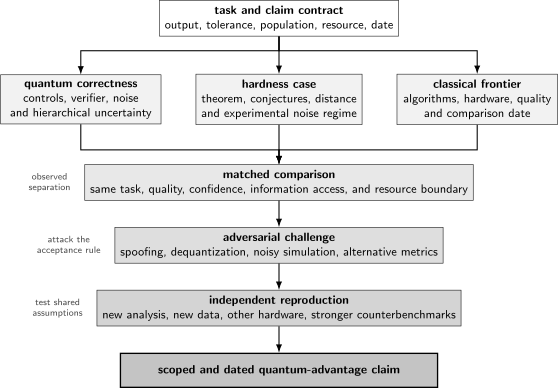
A defensible advantage claim is an evidence chain, not a single score. The task contract fixes what must be produced; correctness tests and hardware controls establish the quantum result; the dated classical frontier supplies the comparator; matched resources and uncertainty establish the observed separation; adversarial challenge and independent reproduction determine how much trust the scoped claim deserves.

Correctness, Hardness, and Superiority

These three layers answer different questions.

Correctness

For instance $x$, let $\mathcal A_\epsilon(x)$ be the accepted-output set. A correctness statement may be

$$\Pr_{\widehat y\sim q_Q(\cdot\mid x)} \left[ \widehat y\in\mathcal A_\epsilon(x) \right] \geq 1-\delta.$$

The probability includes hardware noise, algorithmic randomness, measurement, postprocessing, and any declared retries. Verification may use a direct answer, a certificate, a reference distribution, bounds, conserved quantities, or an interactive challenge.

Hardness

A hardness statement constrains classical algorithms under a model. Its quantifiers matter:

$$\forall a\in\mathfrak C, \qquad C_a(n,\epsilon) \geq L(n,\epsilon),$$

may be a proved lower bound, a conditional consequence of a complexity assumption, or an empirical statement about all methods tried so far. These have different epistemic status.

“Best known classical algorithm costs $C$” is an upper bound on the optimal classical cost:

$$C_C^\star \leq C.$$

It is not a lower bound. No finite benchmark rules out an undiscovered algorithm unless a theorem under a clearly stated model supplies that exclusion.

Superiority

An observed separation compares matched implementations:

$$Q_Q\geq Q_{\min}, \qquad Q_C\geq Q_{\min}, \qquad C_Q<C_C.$$

If the classical method does not attain the required quality within a resource budget $B$, report a censored observation:

$$C_C>B, \qquad \mathcal S_C>\frac{B}{C_Q},$$

not a fabricated runtime. The time limit, quality trajectory, and strongest failed result must be preserved.

Match Verification to the Task

The verification burden depends strongly on the output type.

Decision and function problems

For a decision task with truth $b(x)\in\{0,1\}$, the natural quality is

$$p_{\mathrm{succ}} = \Pr[ \widehat b=b(x) ].$$

Ground truth may come from a certificate, an exact reference for held-out instances, or a construction with known answers. A benchmark should include both yes- and no-instances, difficult boundary cases, and the full confusion matrix when classes are imbalanced.

A theorem such as bounded-error quantum polynomial time concerns an asymptotic error bound. An experiment must still estimate the finite-device success probability and count every repetition required to reach its declared confidence.

Search and witness problems

A search output $y$ can be efficiently verified when

$$V(x,y)=1$$

is cheap to evaluate. Factoring is the standard example: multiplying reported factors is easy even when finding them is believed to be hard. Verification then establishes output correctness but not that the quantum method beat the best classical factoring implementation.

For optimization, feasibility may be easy to check while optimality is hard. The benchmark must distinguish:

$$\text{feasible}, \qquad \text{objective value}, \qquad \text{approximation guarantee}, \qquad \text{certified optimum}.$$

Comparing a quantum feasible point with a classical certified optimum is not a matched task.

Estimation problems

For a target $\theta(x)$ and estimate $\widehat\theta$, declare an error criterion such as

$$\Pr \left[ \left| \widehat\theta-\theta \right| \leq\epsilon \right] \geq 1-\delta.$$

Signed error, bias, variance, mean-squared error, interval width, and empirical coverage answer different questions. The reference value may itself have numerical or experimental uncertainty. If

$$\widehat\theta-\theta_{\mathrm{ref}} = \left( \widehat\theta-\theta \right) + \left( \theta-\theta_{\mathrm{ref}} \right),$$

then agreement with an uncertain reference cannot certify error smaller than the reference uncertainty without additional information.

Sampling problems

A sampler receives an instance $x$ and returns strings from a distribution $q_x$. The ideal target is $p_x$. A strong distributional criterion is

$$\operatorname{TV} \left( p_x,q_x \right) = \frac12 \sum_z \left| p_x(z)-q_x(z) \right| \leq \epsilon.$$

For an alphabet of size $D$, worst-case identity testing against a known distribution requires on the order of

$$\frac{\sqrt D}{\epsilon^2}$$

samples. When $D=2^n$, even sample-efficient identity testing is exponential in $n$. In many advantage proposals, evaluating enough ideal probabilities is also classically expensive.

This creates a verification tension: the output distribution is chosen to be hard to generate classically, but that same hardness can obstruct direct verification. A score

$$T(p_x,q_x) = \mathbb E_{z\sim q_x} \left[ f_x(z) \right]$$

tests one functional $f_x$. Passing it need not imply small total-variation distance. Cross-Entropy Benchmarking gives explicit examples for linear XEB.

Sampling claims should separate:

1. evidence that the device samples from the intended noisy process;
2. evidence that the observed test is difficult to spoof;
3. evidence that close sampling from the intended target is classically hard;
4. an actual resource comparison with current classical methods.

Interactive tasks

An interactive protocol alternates verifier challenges and prover responses. Completeness and soundness have the form

$$\begin{aligned} \Pr[ \text{accept}\mid \text{honest quantum prover} ] &\geq c,\\ \Pr[ \text{accept}\mid \text{allowed classical prover} ] &\leq s, \end{aligned}$$

with gap $c-s>0$. Repetition can amplify the gap, but communication, verifier work, cryptographic setup, and assumptions must be counted. Efficient verification does not mean assumption-free verification.

The Complexity Evidence

Complexity theory explains why a task is a plausible advantage candidate. It does not replace experimental verification.

Exact and approximate hardness

For selected circuit families, exact output amplitudes or probabilities encode $\#\mathrm P$-hard quantities. Experimental samplers, however, are noisy and approximate. A result about exact computation does not automatically imply hardness of sampling within constant total-variation distance.

The standard conditional route for random sampling has several links:

1. identify a worst-case hard counting quantity;
2. conjecture or prove suitable average-case hardness for random instances;
3. establish anticoncentration so additive approximation is informative;
4. use approximate counting arguments to connect an efficient classical sampler to consequences such as collapse of the polynomial hierarchy;
5. show that the experimental noise and score place the device in the regime covered by that argument.

Each arrow has conditions. Different sampling proposals establish different subsets of the chain. The phrase “classically hard by complexity theory” should be replaced by the exact theorem, conjecture, distance measure, and noise regime.

Worst case is not average case

A worst-case lower bound says that some instances are difficult:

$$\max_{x\in\mathcal X_n} C_C(x) \geq L(n).$$

An experiment draws from $\Pi_n$ and needs a statement about typical or quantile cost:

$$\Pr_{x\sim\Pi_n} \left[ C_C(x)\geq L_\alpha(n) \right] \geq 1-\alpha.$$

Choosing only high-cost instances after inspecting a classical simulator changes $\Pi_n$. If hard-instance selection is part of the task, its search cost and information leakage belong in the contract.

Oracle and communication separations

Query, sample, and communication lower bounds can be unconditional within their models. They are powerful because the compared information interfaces are explicit. They can also hide physical costs. A quantum state supplied as one sample is not equivalent to a classical list, and a coherent oracle query is not equivalent to a database lookup.

The advantage claim should therefore preserve the theorem’s interface:

$$\text{formal access model} \longrightarrow \text{physical preparation} \longrightarrow \text{measured resource}.$$

If the middle arrow costs exponentially more than one abstract query, the formal separation may not survive end to end.

Build a Dated Classical Frontier

The classical comparator is part of the experiment, not a citation selected afterward.

Classical Information Review supplies the fixed source–channel–code–decoder, access, error, and cost ledger. This page adds the dated algorithm portfolio, matched resources, superiority test, and independent challenge needed for a quantum-advantage claim.

A frontier, not one code

Let $\mathcal A_C(t_0)$ be the credible classical algorithms available by date $t_0$. The empirical quality–cost frontier is

$$Q_C^\star(B;t_0) = \sup_{ a\in\mathcal A_C(t_0): C_a\leq B } Q_a.$$

A quantum point $(B_Q,Q_Q)$ lies beyond that measured frontier only if

$$Q_Q > Q_C^\star(B_Q;t_0)$$

with uncertainty and selection effects included. This statement is more durable than comparing two headline runtimes because it preserves partial classical progress.

The baseline portfolio should include:

• a simple transparent method;
• competitive domain-specific algorithms;
• state-of-the-art simulation, approximation, or heuristic methods;
• hardware-accelerated and distributed variants when relevant;
• algorithms designed to target the verifier rather than the full ideal object;
• lower-cost methods with different quality–resource tradeoffs;
• independent implementations when software quality could determine the result.

Match information and accuracy

Both sides must receive equivalent input information and return the same object. A classical algorithm asked to reconstruct a full probability distribution is not matched to a quantum device asked for samples. A quantum estimator given coherent state access is not matched to a classical method given only individual measurement outcomes unless that access asymmetry is the theorem being tested.

Accuracy includes confidence:

$$\left( \epsilon_Q, \delta_Q \right) = \left( \epsilon_C, \delta_C \right)$$

or both must satisfy a common threshold. Comparing medians at unequal tail risk can reverse time-to-solution rankings.

Match resources and boundaries

For each baseline report:

• source code, version, numerical precision, libraries, and compiler;
• processor, accelerator, memory, interconnect, storage, and parallelism;
• preprocessing, contraction-order search, training, caching, and tuning;
• wall-clock time, peak memory, energy, and monetary policy where claimed;
• failed and censored runs;
• output quality and verification cost;
• date and enough artifacts to rerun the comparison.

Peak floating-point operations and hardware list prices are not measured runtime or cost. A projected classical runtime can support a conditional claim, but it should not be described as an executed baseline.

Classical progress is part of the result

Classical counterbenchmarks often exploit structure omitted by a generic estimate: circuit geometry, low effective entanglement, favorable contraction orders, batched amplitudes, low target fidelity, symmetries, noise, or the specific acceptance statistic. These are legitimate unless the task contract forbids them for a reason applied symmetrically to the quantum method.

Define a baseline revision factor

$$\rho_C(t_1,t_0) = \frac{ C_C^\star(t_0) }{ C_C^\star(t_1) }, \qquad t_1>t_0.$$

If $\rho_C>1$, the classical frontier improved. The original measurement has not changed, but the present-tense advantage ratio has:

$$\mathcal S_C(t_1) = \frac{ \mathcal S_C(t_0) }{ \rho_C(t_1,t_0) }.$$

This is why durable prose says “exceeded the evaluated classical frontier under the 2019 comparison” rather than converting a dated experiment into an atemporal theorem.

Spoofing and Dequantization

An honest reference implementation and an adversary targeting the acceptance test solve different problems.

Suppose the verifier accepts when

$$T(q)\geq\tau.$$

The intended task may be to sample close to $p$, but a spoofing algorithm only needs to find any $q_{\mathrm{sp}}$ satisfying

$$T(q_{\mathrm{sp}})\geq\tau$$

at low cost. If

$$\operatorname{TV} \left( q_{\mathrm{sp}},p \right) \gg\epsilon,$$

the test has accepted the wrong object. The correct repair is to narrow the claim, strengthen the test battery, or change the protocol. It is not enough to observe that the spoofing algorithm behaves unlike the intended quantum process.

Dequantization asks whether the mathematical idea behind a quantum algorithm can be reproduced classically after matching data access and output requirements. Quantum-inspired linear algebra, tensor networks, stabilizer decompositions, low-rank approximations, and problem-specific heuristics can all alter the comparison. A serious advantage program invites these attacks before freezing the claim.

Quantum Machine Learning owns QML-family access assumptions and dequantization results; this page retains the general adversarial validation framework.

An adversarial audit should ask:

1. Can a classical method optimize the published scalar without reproducing the target?
2. Can noise simplify the generated distribution?
3. Can instance structure, low depth, sparsity, or symmetry be exploited?
4. Can preprocessing be amortized across requested samples?
5. Can an approximate answer satisfy the actual acceptance rule?
6. Can a quantum-inspired method use the same data-access assumption?
7. Can a stronger verifier be evaluated on hidden instances?

Publishing successful classical attacks is part of validating the boundary, not a failure of quantum science.

Hardware Noise Can Change the Computational Problem

Let the ideal target be $p_x$ and the physical distribution be

$$q_x = \mathcal N_x[p_x],$$

where $\mathcal N_x$ denotes the complete noisy implementation. The relevant hardness question is not only whether $p_x$ is hard to sample. It is whether a classical algorithm can reproduce the accepted properties of $q_x$ or the specified tolerance around $p_x$.

At sufficiently high noise, a circuit may approach a simple distribution:

$$q_x \longrightarrow u,$$

where $u$ is uniform or another efficiently sampled fixed point. More generally, local noise can reduce entanglement or magic enough for a specialized simulator to become efficient. Increasing qubit count does not restore hardness if the usable signal decays faster than classical cost grows.

The experiment should therefore report:

• a calibrated noise and leakage description;
• quality versus width, depth, and time;
• evidence connecting tractable validation circuits to target circuits;
• simulator performance on the noisy, not only ideal, task;
• drift and calibration epochs;
• whether the hardness argument tolerates the measured error model.

Postselection

For acceptance event $A$, the reported conditional distribution is

$$q_A(z) = q(z\mid A),$$

with acceptance probability

$$a = \Pr(A).$$

If one accepted result requires geometric retries, the expected raw count is

$$\mathbb E[N_{\mathrm{raw}}] = \frac{ N_{\mathrm{accepted}} }{ a }.$$

A high-quality $q_A$ at exponentially small $a$ does not establish an efficient unconditional task. The verifier must also check that conditioning did not redefine the problem by discarding hard instances or unfavorable outputs.

Error mitigation

An error-mitigated estimator can be written schematically as

$$\widehat\theta_{\mathrm{mit}} = \sum_{j=1}^m w_j \widehat\theta_j.$$

Its variance is approximately

$$\operatorname{Var} \left( \widehat\theta_{\mathrm{mit}} \right) = \sum_{j,k} w_jw_k \operatorname{Cov} \left( \widehat\theta_j, \widehat\theta_k \right).$$

Large signed weights can produce substantial sampling overhead, while model mismatch can leave bias. Probabilistic Error Cancellation owns the implemented signed-weight, model-mismatch, validation, and total-resource audit for that estimator family. Count every noise-scaled circuit, calibration, rejected shot, and classical fit. Mitigation can improve correctness evidence; it does not make the classical comparator, dated classical frontier, or hardness argument unnecessary.

A Verification Ladder

No universal protocol simultaneously gives low-cost, assumption-free, device-independent verification of every hard quantum computation. Use the strongest combination available for the task.

method	what it establishes	scaling or assumption limit
exact classical reference	direct output or probability comparison	usually restricted to small width, depth, or structure
tractable subfamilies	implementation correctness on controlled cases	extrapolation to target instances needs validation
efficient witness or certificate	correctness of each accepted answer	unavailable for many sampling and optimization tasks
bounds and conserved quantities	consistency with necessary physical relations	necessary conditions need not identify the full state
randomized cross-platform tests	selected overlaps, moments, or local properties	trust and sample assumptions; not complete equivalence
interactive or cryptographic protocol	completeness–soundness gap against a defined prover	cryptographic assumptions, communication, and circuit overhead
hidden challenge instances	reduces tuning and verifier targeting	generator and secrecy policy become trusted components
independent reproduction	robustness across teams, code, and hardware	shared assumptions can survive replication

Overlap regime

Choose sizes for which independent exact or converged methods are available. Validate not only final scores but intermediate distributions, marginals, amplitudes, observables, and error models. An overlap study supports extrapolation only when residuals and model parameters remain stable as size increases.

Tractable deformations

Useful controls include reduced depth, lower width, removable gates, Clifford limits, integrable limits, low-entanglement instances, known symmetries, and circuits with planted answers. Randomize their placement among target instances so calibration drift cannot masquerade as scale dependence.

A deformation parameter $\lambda$ can define a validation path:

$$\mathcal P(0) = \mathcal P_{\mathrm{tractable}}, \qquad \mathcal P(1) = \mathcal P_{\mathrm{target}}.$$

Agreement near $\lambda=0$ does not prove correctness at $\lambda=1$. Measure the breakdown of each validation method and avoid extrapolating across an unexplained regime change.

Certificates and interaction

Search problems with efficiently checked witnesses are favorable because generation can be hard while verification remains easy. Interactive and cryptographic protocols can create a completeness–soundness gap even when direct simulation is unavailable. Their security statement is only as strong as the prover model, cryptographic assumption, verifier implementation, and randomness source.

Cross-checks

Different tests should fail differently. Combine local observables, global scores, conservation laws, reverse or mirror circuits, randomized measurements, independent simulators, and hardware sentinels. Agreement among correlated tests is weaker than agreement among methods with distinct representations and failure modes.

Statistical Evidence for a Separation

An advantage statement is an inference over instances, runs, and time, not the difference between two stopwatch readings.

Define the estimand

For a positive scalar cost, a convenient paired effect is the log speedup

$$\ell_i = \log C_{C,i} - \log C_{Q,i}$$

on matched instance $i$. The population effect is

$$\Delta = \mathbb E_{x\sim\Pi} \left[ \ell(x) \right].$$

Then $\Delta>0$ means geometric-mean quantum advantage under the declared cost and population. This does not imply that every instance favors the quantum method. Report the distribution of $\ell_i$, tail quantiles, and the fraction of instances with $\ell_i>0$.

A one-sided test can use

$$H_0:\Delta\leq0, \qquad H_1:\Delta>0.$$

Under a regular large-sample approximation, evidence for a positive effect requires

$$\widehat\Delta - z_{1-\alpha} \operatorname{SE} \left( \widehat\Delta \right) > 0.$$

Equivalently, the lower confidence bound on the geometric speedup exceeds one:

$$\exp \left[ \widehat\Delta - z_{1-\alpha} \operatorname{SE} \left( \widehat\Delta \right) \right] > 1.$$

Runtime distributions are often skewed, heavy-tailed, or censored by time limits. Paired bootstrap intervals, survival-analysis methods, or hierarchical models may be preferable to a Gaussian approximation. Preserve timeout events instead of replacing them by the timeout value without qualification.

Use the right sampling unit

Shots from one circuit do not create independent circuit instances. Repeated circuits in one calibration epoch do not create independent device epochs. A useful hierarchy is

$$\text{instance family} \supset \text{instance} \supset \text{time block} \supset \text{execution} \supset \text{shot}.$$

Uncertainty should reflect every level over which the conclusion generalizes. If the claim concerns fresh random instances and future operating periods, shot-only error bars are inadequate.

Use paired designs when possible: quantum and classical methods receive the same instance, tolerance, random seed policy, and budget. Randomize acquisition order, retain timestamps, and block by calibration epoch. Keep the held-out test set separate from algorithm, compiler, and mitigation tuning.

Separate statistical and practical significance

A very precise ratio of $1.002$ may be statistically positive but operationally irrelevant. Define a minimum consequential advantage $\Delta_{\min}$:

$$H_0: \Delta\leq\Delta_{\min}.$$

For practical claims, $\Delta_{\min}$ should reflect service latency, reliability, energy, cost, or downstream value. For a foundational demonstration, any reproducible finite separation may be scientifically important, but its scope should remain foundational.

Control selection and optional stopping

Trying many qubit subsets, circuit families, depths, scores, mitigation settings, classical baselines, and stopping times creates a selection problem. If $K$ prespecified independent hypotheses are tested with familywise error target $\alpha$, a simple conservative threshold is

$$\alpha_{\mathrm{local}} = \frac{\alpha}{K}.$$

Dependence-aware corrections or hierarchical models can be more powerful, but the selection policy must be declared. Sequential tests require an alpha spending rule, confidence sequence, or other valid stopping procedure. Stopping when the speedup first crosses one and then using a fixed-sample interval exaggerates evidence.

A p-value cannot quantify undiscovered algorithms

A p-value can test a statistical null about data generated by specified models. It cannot assign a probability that no faster classical algorithm exists. The uncertainty in the classical frontier includes epistemic uncertainty about algorithms, implementations, extrapolations, and future progress. Report that separately from sampling uncertainty.

End-to-End Resource Accounting

Algorithmic Benchmarking develops the full resource ledger. For an advantage claim, the key rule is symmetry: include or exclude the same class of work on both sides and publish the boundary.

For a quantum workflow,

$$\begin{aligned} T_Q =\;& T_{\mathrm{input}} + T_{\mathrm{prepare}} + T_{\mathrm{compile}}\\ &+ T_{\mathrm{queue}} + T_{\mathrm{execute}} + T_{\mathrm{feedback}}\\ &+ T_{\mathrm{readout}} + T_{\mathrm{post}} + T_{\mathrm{verify}}. \end{aligned}$$

Queue time may be excluded from a hardware-throughput claim and included in a service-latency claim. Both can be legitimate if named. Classical accelerator startup, data movement, contraction-order search, checkpointing, and output verification deserve the same treatment.

If each full trial succeeds independently with probability $p_{\mathrm{sol}}$, then

$$\mathbb E[N_{\mathrm{trial}}] = \frac1{p_{\mathrm{sol}}},$$

and a simple expected time-to-solution model is

$$\mathbb E[T_{\mathrm{sol}}] = T_{\mathrm{setup}} + \frac{ T_{\mathrm{trial}} }{ p_{\mathrm{sol}} } + T_{\mathrm{verify}}.$$

This formula must be modified for adaptive retries, nonstationarity, shared setup, parallel execution, or heavy-tailed completion times.

Amortization

For $K$ related tasks, write

$$T_Q(K) = T_{Q,0} + K T_{Q,\mathrm{marg}},$$

and similarly for the classical method. If

$$T_{Q,\mathrm{marg}} < T_{C,\mathrm{marg}},$$

but $T_{Q,0}>T_{C,0}$, the crossover workload is

$$K_\star = \frac{ T_{Q,0}-T_{C,0} }{ T_{C,\mathrm{marg}}-T_{Q,\mathrm{marg}} }.$$

A one-shot comparison can miss a genuine batched advantage, while an amortized claim can hide a setup cost that real users rarely recover. State the workload volume and cache lifetime.

Energy and monetary cost

Energy advantage requires metering comparable system boundaries. Processor power alone omits cryogenics, lasers, vacuum, control electronics, networking, and data-center overhead. Classical thermal-design power is not measured energy. Monetary comparisons depend on utilization, depreciation, cloud pricing, labor, and subsidy. They are valid only as dated economic scenarios, not intrinsic properties of quantum mechanics.

Three Historical Case Audits

Case studies are useful because each exposes a different weak link. They are not permanent leaderboards.

Random-circuit sampling

The 2019 Sycamore experiment executed random circuits on a 53-qubit superconducting processor, evaluated linear-XEB correlations on verifiable subsets, and compared the sampling time with then-current classical estimates. The experiment established a large-scale programmable random-circuit execution and a finite comparison under its stated model.

The full claim combined:

1. conditional complexity evidence for approximate random-circuit sampling;
2. hardware calibration and XEB-based correctness evidence;
3. extrapolation from classically verifiable circuits;
4. a classical simulation cost estimate;
5. an observed quantum sampling rate.

Later tensor-network and batched-amplitude algorithms substantially revised parts of the classical-cost landscape, and explicit algorithms showed that some scalar XEB targets can be spoofed without faithful sampling. Subsequent experiments and theory also identified depth-and-noise regimes separated by sharp changes in XEB behavior and simulability.

The durable lesson is not that the original device data disappeared or that all random-circuit advantage claims are equivalent. It is that the result must be indexed by circuit ensemble, score, target fidelity, classical algorithm, hardware, and date. A present claim needs a present counterbenchmark.

Photonic sampling

Gaussian boson-sampling experiments such as Jiuzhang and Borealis produced large photon-counting data sets from programmable optical networks and reported comparisons with classical generation methods. Relevant physical deviations include loss, partial distinguishability, detector noise, mode mismatch, and source imperfections.

Validation commonly combines low-order correlators, likelihood ratios, heavy-output or cross-entropy-like statistics, tractable reduced instances, and calibrated device models. None alone identifies an exponentially large distribution. Classical algorithms may target the validation statistic, exploit loss, or approximate only the quality actually required.

The verification contract should therefore distinguish:

$$\text{ideal boson sampling}, \qquad \text{calibrated noisy optical model}, \qquad \text{observed samples}.$$

A hardness theorem for the first object, a fit of the second, and data from the third are complementary evidence, not interchangeable proof.

Many-body quantum simulation

The 2023 127-qubit kicked-Ising experiment reported mitigated expectation values beyond brute-force state-vector simulation and carefully used the language “evidence for utility.” It compared against several tensor-network methods available during the study.

Independent 2024 work developed geometry-aware and converged tensor-network calculations that reproduced or improved reference results in substantial parts of the studied regime. This did not retroactively change the quantum measurements. It strengthened the classical frontier and narrowed which observables and regimes remained beyond specific methods.

This case illustrates why:

• failure of brute force is not failure of classical computation;
• several classical representations should be tested;
• convergence evidence is as important as nominal system size;
• mitigated quantum error bars need bias analysis;
• “evidence for utility” is not automatically a computational-advantage theorem.

An independent classical success is valuable scientific information because it reveals structure in the state and improves future benchmark design.

Verifiable Advantage Protocols

An attractive protocol makes generation hard and checking easy. Several research directions pursue this alignment.

Cryptographic tests of quantumness

Trapdoor claw-free constructions can let a classical verifier challenge a single quantum prover. Under assumptions such as the classical hardness of learning with errors, the prover’s responses exhibit a completeness–soundness gap unavailable to efficient classical strategies. Computational Bell-test proposals trade circuit fidelity against repeated trials while retaining efficient classical verification.

These protocols replace direct simulation by cryptographic soundness. They must still validate:

• key generation and trapdoor secrecy;
• the precise classical adversary model;
• quantum circuit depth and reversible arithmetic;
• postselection and repetition overhead;
• verifier randomness and implementation;
• finite-sample rejection of the classical bound.

A cryptographic proof is conditional in a useful and explicit way. It should not be described as device independent when its security relies on computational assumptions and trusted classical components.

Blind and Delegated Quantum Computation separates this integrity question from privacy. It develops simulator-based blindness, accepted-wrong-output bounds, weak quantum clients, classical verifiers, and the leakage and availability limits of private delegation.

Self-verifying sampling structures

Bell sampling from two circuit copies has been proposed as a universal computational model whose samples also reveal selected circuit properties, including fidelity-related and complexity diagnostics. Other work develops peaked distributions or sample-complexity tasks for which outputs are easier to verify than flat random-circuit samples.

For example, the 2026 complement-sampling result proves a strong quantum sample-complexity separation and develops average-case and verifiability properties under stated assumptions. It is a theoretical protocol and candidate experimental route, not by publication alone a hardware demonstration.

The active design objective is:

$$\begin{aligned} \text{quantum generation cost} &\ll \text{classical generation cost},\\ \text{verification cost} &\ll \text{classical generation cost}. \end{aligned}$$

Achieving both inequalities at useful physical scale remains a central research problem.

Independent Reproduction

“Reproduced” should name what was repeated. Four levels are useful.

Artifact reproduction

An independent team reruns the released analysis, circuits, classical baselines, and figures from the same raw data. This detects undocumented software, environment, and analysis choices.

Result reproduction

The team repeats the protocol on the same hardware service or apparatus with new data and frozen rules. This tests time stability but may share firmware, calibration, and institutional assumptions.

Cross-platform replication

A different device or architecture executes the same task contract and acceptance rule. Exact circuit matching may be inappropriate across platforms; the logical task, information access, quality, and resource boundaries should remain fixed.

Independent challenge

Specialists develop new classical algorithms, spoofing strategies, dequantizations, error models, and statistical analyses without being restricted to the original baseline portfolio. This is the strongest test of the claimed boundary and often changes it.

Reproduction confidence grows when teams differ in hardware, software, funding, representation, and method. Several papers using the same simulator or calibration model are not fully independent.

Minimum reusable artifacts include:

• instance generators, seeds, logical and compiled circuits;
• pulse or control metadata when material;
• raw outcomes with timestamps and calibration identifiers;
• inclusion, postselection, and retry records;
• all score and uncertainty code;
• classical baseline source, build instructions, parameters, and logs;
• hardware, memory, accelerator, energy, and timing records;
• exact figure and table generation environments;
• a machine-readable claim contract.

Reproducible Notebooks develops the executable evidence bundle.

A Defensible Workflow

1. Name the claim type. State model, asymptotic, finite experimental, or practical advantage and the resource being compared.
2. Freeze the task. Specify inputs, promises, outputs, tolerance, confidence, instance population, and access model.
3. Freeze the verifier. Define every score, threshold, hidden challenge, reference calculation, and failure rule before inspecting target results.
4. Map the hardness chain. Label proved reductions, average-case conjectures, anticoncentration assumptions, noise conditions, and open arrows.
5. Validate the quantum implementation. Use overlap instances, tractable deformations, hardware controls, drift sentinels, and independent tests.
6. Build a classical portfolio. Include transparent, domain-specific, state-of-the-art, approximate, hardware-accelerated, and verifier-targeting methods.
7. Match boundaries. Equalize input information, output quality, confidence, preprocessing, amortization, failures, and verification.
8. Freeze tuning. Separate development from held-out evaluation for both quantum and classical methods.
9. Run hierarchical repetitions. Sample instances, seeds, time blocks, executions, and shots at the levels the claim generalizes over.
10. Report the frontier. Publish quality–cost curves, censored runs, uncertainty, and Pareto tradeoffs rather than only the winning point.
11. Invite adversarial challenge. Test spoofing, dequantization, noisy simulation, hidden structure, and alternative statistical analyses.
12. Reproduce independently. Repeat artifacts, data acquisition, platforms, and classical counterbenchmarks where feasible.
13. Date and scope the conclusion. Name exactly which frontier was crossed and what remains conjectural or unverified.
14. Schedule reassessment. Recompute the comparison when algorithms, hardware, verification methods, or the task definition changes.

Minimum Reporting Record

field	required content
claim	exact advantage type, resource, scope, and date
task	problem, instance distribution, promises, inputs, outputs, and access
success	score or loss, tolerance, confidence, failures, retries, and postselection
quantum method	algorithm, hardware, compiler, controls, calibration epoch, mitigation, and raw data
correctness	verifier, references, overlap regime, controls, model assumptions, and uncertainty
hardness	theorem, conjecture, worst- or average-case scope, approximation norm, and noise regime
classical frontier	algorithms, versions, tuning, hardware, precision, quality, timeouts, and date
resources	complete time, memory, energy, parallelism, samples, and amortization boundaries
statistics	sampling unit, hierarchy, pairing, intervals, multiplicity, stopping, and practical threshold
adversarial tests	spoofing, dequantization, noisy simulation, alternative metrics, and negative results
reproduction	artifacts, independent analyses, new data, platforms, and unresolved discrepancies
conclusion	narrow statement supported by all three layers and explicit exclusions

Common Mistakes

Calling a benchmark score an advantage

A score establishes performance on its protocol. Advantage additionally needs correctness, hardness, and a matched classical frontier.

Treating a classical runtime estimate as a lower bound

The cost of one algorithm is an upper bound on optimal classical cost. Label projections and execute strong baselines where feasible.

Comparing different outputs

Samples, selected amplitudes, full distributions, expectation values, and certified answers are different tasks.

Using ideal hardness for a noisy distribution

Noise can simplify the physical output. Analyze the accepted noisy task and the distance to the ideal target.

Verifying only easy circuits

Reduced circuits are valuable controls, but extrapolation to the target needs a validated model and uncertainty.

Optimizing the verifier on public test data

A published scalar may be spoofable. Use held-out tests, multiple functionals, and adversarial baseline design.

Counting only accepted shots

Postselection changes both distribution and cost. Report unconditional success and all rejected attempts.

Ignoring classical tuning

Contraction-order search, training, compilation, and preprocessing are costs, but denying classical methods a tuning budget while optimizing the quantum stack is asymmetric.

Using shot error bars for a population claim

Generalization over instances, seeds, and calibration epochs requires uncertainty at those levels.

Converting a conditional theorem into an experimental proof

Average-case hardness, anticoncentration, cryptographic assumptions, and noise tolerance must be named.

Treating independent analysis as independent hardware replication

Both are useful and answer different questions. State which layer was reproduced.

Treating the baseline date as irrelevant

An empirical separation can narrow when a new classical algorithm appears. Preserve the historical result and update present-tense claims.

Equating advantage with usefulness

A contrived sampling separation may be foundationally important without solving an end-user problem.

Research Status

Established: task matching, explicit access models, complete resource boundaries, uncertainty, dated baselines, and independent reproduction are durable requirements of scientific advantage claims. Verification and classical simulation are distinct activities. A benchmark score alone does not establish computational advantage.

Active: scalable correctness tests, verifier-resistant sampling protocols, noise-aware hardness, fair energy accounting, hidden-instance governance, logical-machine comparisons, and independent cross-platform replication remain active research. Classical and quantum frontiers continue to move.

Conjectural: many approximate random-sampling hardness arguments depend on average-case complexity and anticoncentration conjectures. The conditions under which realistic noise preserves intractability are protocol dependent and not settled by one universal theorem.

Speculative: projections from current devices to broad practical advantage depend on future error correction, algorithms, data interfaces, hardware costs, and classical progress. They should be presented as scenarios, not experimental conclusions.

Terminology is not fully standardized. “Advantage,” “utility,” “beyond classical,” “quantumness,” and “practical advantage” can encode different tasks and evidence thresholds. The claim contract matters more than the label.

Further Connections

• Algorithmic Benchmarking supplies task acceptance, hybrid-loop, retry, scaling, and cost-to-solution accounting.
• Cross-Entropy Benchmarking develops the random-circuit statistic, reference bottleneck, fidelity assumptions, total-variation gap, and spoofing literature.
• Why Benchmarking Is Hard develops estimands, drift, selection, verification ladders, and reporting logic for benchmarks generally.
• Reporting Standards provides the advantage-claim profile, immutable evidence lineage, matched resource boundaries, artifact identity, and correction policy.
• Quantum Complexity Classes distinguishes BQP evidence, oracle separations, promise problems, and unproved class separations.
• Quantum Circuit Simulation compares exact, hybrid, and approximate classical simulators.
• Tensor-Network Simulation develops contraction costs, truncation controls, convergence, and circuit-geometry dependence.
• Negative Results and Limitations records dated classical reversals, nulls, lower bounds, and unresolved bridges without turning them into field-wide impossibility claims.
• Noise Simulation shows how noise models alter the task a classical simulator must reproduce.
• Noise in Quantum Information distinguishes stochastic, coherent, leakage, correlated, non-Markovian, and drift effects.
• Resource Estimation Tools owns conditional projections for future fault-tolerant algorithms.
• Claims, Hype, and Evidence Standards supplies the broader theorem, experiment, benchmark, estimate, and application taxonomy.
• Reproducible Notebooks specifies executable artifacts and provenance.
• Validation Tests collects reusable checks for computational evidence.

References

1. D. Hangleiter and J. Eisert, “Computational advantage of quantum random sampling,” Reviews of Modern Physics 95, 035001 (2023), doi:10.1103/RevModPhys.95.035001.
2. T. Proctor, K. Young, A. D. Baczewski, and R. Blume-Kohout, “Benchmarking quantum computers,” Nature Reviews Physics 7, 105–118 (2025), doi:10.1038/s42254-024-00796-z.
3. S. Aaronson and L. Chen, “Complexity-theoretic foundations of quantum supremacy experiments,” in Proceedings of the 32nd Computational Complexity Conference, 22:1–22:67 (2017), doi:10.4230/LIPIcs.CCC.2017.22.
4. A. Bouland, B. Fefferman, C. Nirkhe, and U. Vazirani, “On the complexity and verification of quantum random circuit sampling,” Nature Physics 15, 159–163 (2019), doi:10.1038/s41567-018-0318-2.
5. F. Arute et al., “Quantum supremacy using a programmable superconducting processor,” Nature 574, 505–510 (2019), doi:10.1038/s41586-019-1666-5.
6. F. Pan, K. Chen, and P. Zhang, “Solving the sampling problem of the Sycamore quantum circuits,” Physical Review Letters 129, 090502 (2022), doi:10.1103/PhysRevLett.129.090502.
7. X. Gao, M. Kalinowski, C.-N. Chou, M. D. Lukin, B. Barak, and S. Choi, “Limitations of linear cross-entropy as a measure for quantum advantage,” PRX Quantum 5, 010334 (2024), doi:10.1103/PRXQuantum.5.010334.
8. A. Morvan et al., “Phase transitions in random circuit sampling,” Nature 634, 328–333 (2024), doi:10.1038/s41586-024-07998-6.
9. H.-S. Zhong et al., “Quantum computational advantage using photons,” Science 370, 1460–1463 (2020), doi:10.1126/science.abe8770.
10. L. S. Madsen et al., “Quantum computational advantage with a programmable photonic processor,” Nature 606, 75–81 (2022), doi:10.1038/s41586-022-04725-x.
11. C. Oh, L. Jiang, and B. Fefferman, “Spoofing cross-entropy measure in boson sampling,” Physical Review Letters 131, 010401 (2023), doi:10.1103/PhysRevLett.131.010401.
12. J. Eisert et al., “Quantum certification and benchmarking,” Nature Reviews Physics 2, 382–390 (2020), doi:10.1038/s42254-020-0186-4.
13. J. Carrasco, A. Elben, C. Kokail, B. Kraus, and P. Zoller, “Theoretical and experimental perspectives of quantum verification,” PRX Quantum 2, 010102 (2021), doi:10.1103/PRXQuantum.2.010102.
14. A. Gheorghiu, T. Kapourniotis, and E. Kashefi, “Verification of quantum computation: an overview of existing approaches,” Theory of Computing Systems 63, 715–808 (2019), doi:10.1007/s00224-018-9872-3.
15. D. Hangleiter, M. Kliesch, J. Eisert, and C. Gogolin, “Sample complexity of device-independently certified ‘quantum supremacy’,” Physical Review Letters 122, 210502 (2019), doi:10.1103/PhysRevLett.122.210502.
16. G. D. Kahanamoku-Meyer, S. Choi, U. V. Vazirani, and N. Y. Yao, “Classically verifiable quantum advantage from a computational Bell test,” Nature Physics 18, 918–924 (2022), doi:10.1038/s41567-022-01643-7.
17. Z. Brakerski, P. Christiano, U. Mahadev, U. Vazirani, and T. Vidick, “A cryptographic test of quantumness and certifiable randomness from a single quantum device,” Journal of the ACM 68, article 31 (2021), doi:10.1145/3441309.
18. D. Hangleiter and M. J. Gullans, “Bell sampling from quantum circuits,” Physical Review Letters 133, 020601 (2024), doi:10.1103/PhysRevLett.133.020601.
19. M. Benedetti, H. Buhrman, and J. Weggemans, “Provable and verifiable quantum advantage in sample complexity,” Physical Review Letters 136, 040601 (2026), doi:10.1103/q55v-wm7y.
20. Y. Kim et al., “Evidence for the utility of quantum computing before fault tolerance,” Nature 618, 500–505 (2023), doi:10.1038/s41586-023-06096-3.
21. J. Tindall, M. Fishman, E. M. Stoudenmire, and D. Sels, “Efficient tensor network simulation of IBM’s Eagle kicked Ising experiment,” PRX Quantum 5, 010308 (2024), doi:10.1103/PRXQuantum.5.010308.
22. T. Begušić, J. Gray, and G. K.-L. Chan, “Fast and converged classical simulations of evidence for the utility of quantum computing before fault tolerance,” Science Advances 10, eadk4321 (2024), doi:10.1126/sciadv.adk4321.
23. T. Hoefler, T. Häner, and M. Troyer, “Disentangling hype from practicality: on realistically achieving quantum advantage,” Communications of the ACM 66, 82–87 (2023), doi:10.1145/3571725.
24. S. Ferracin, S. T. Merkel, D. McKay, and A. Datta, “Experimental accreditation of outputs of noisy quantum computers,” Physical Review A 104, 042603 (2021), doi:10.1103/PhysRevA.104.042603.
25. A. Elben et al., “Cross-platform verification of intermediate scale quantum devices,” Physical Review Letters 124, 010504 (2020), doi:10.1103/PhysRevLett.124.010504.

Exercises

1. Separate the three propositions

A processor produces samples with positive linear XEB on 60-qubit circuits. The score is statistically different from zero. Identify what this establishes and what remains to support a computational-advantage claim.

Solution

The measurement establishes correlation with ideal probabilities under the reported XEB convention, subject to reference and statistical checks. Under a validated scrambling-and-noise model it may also estimate an effective circuit fidelity.

Correctness still needs evidence that the compiled target was executed and that the score supports the intended output claim. Hardness needs a protocol-specific argument for approximate sampling in the measured depth-and-noise regime. Superiority needs a dated classical portfolio using the same circuits, score, target fidelity, sample count, and resources. Spoofing tests, hidden instances, complete timing, and independent analysis remain necessary. Positive XEB alone does not establish small total-variation distance or advantage.

2. Compute a confidence bound on speedup

On paired held-out instances, the estimated geometric-mean speedup is $5$. The standard errors of mean log classical and quantum costs are $0.12$ and $0.08$, and their covariance is negligible. Compute an approximate 95% one-sided lower bound on the speedup using $z_{0.95}=1.645$.

Solution

The log effect is

$$\widehat\Delta = \log 5 \approx 1.609.$$

Its standard error is

$$\operatorname{SE} \left( \widehat\Delta \right) = \sqrt{ 0.12^2+0.08^2 } \approx 0.144.$$

The lower log bound is

$$1.609 - 1.645(0.144) \approx 1.372.$$

Therefore the lower speedup bound is

$$e^{1.372} \approx 3.94.$$

Under the stated approximation, the data support at least a $3.9$-fold geometric-mean separation for the tested population and comparison contract. Instance hierarchy, censoring, and classical-frontier uncertainty still need separate checks.

3. Charge postselection

A sampling protocol accepts $2\%$ of raw trials and requests $10\,000$ accepted outputs. How many raw trials are expected? What must be included in a runtime comparison?

Solution

With $a=0.02$,

$$\mathbb E[N_{\mathrm{raw}}] = \frac{ 10\,000 }{ 0.02 } = 500\,000.$$

The quantum cost includes all rejected trials, reset, preparation, measurement, selection, communication, and verification. The report must publish both the conditional output quality and the acceptance probability. The classical comparator must produce the same accepted-output object under the same rule; otherwise the tasks differ.

4. Find an amortization crossover

A quantum service has setup time $1000$ s and marginal time $2$ s per task. A classical service has setup time $100$ s and marginal time $10$ s. At what integer workload size does the quantum service first become faster?

Solution

Solve

$$1000+2K < 100+10K.$$

Thus

$$900 < 8K, \qquad K > 112.5.$$

The first integer crossover is $K=113$. A defensible claim must also match quality, reliability, parallelism, cache lifetime, and verification cost. It should say “batched runtime advantage for at least 113 tasks under this scenario,” not simply “the quantum service is faster.”

5. Audit a sampling verifier

A verifier accepts any sampler whose mean value of one published statistic exceeds $\tau$. A classical algorithm outputs only strings known to score highly and passes, although its distribution is far from the ideal target. Which proposition failed, and how can the protocol be repaired?

Solution

The test did not identify the intended output object. It established only the one-dimensional statistic, so the correctness proposition for close sampling failed. The classical algorithm is a valid spoofing counterexample to the published verifier.

Repairs include narrowing the claim to the statistic, adding held-out and secret tests, using several diagnostics with different failure modes, choosing a protocol with certificates or interaction, and proving a stronger connection between acceptance and the target distance. The cost and security assumptions of the strengthened verifier must be included.

6. Label a hardness chain

A proposal proves worst-case exact amplitude computation is $\#\mathrm P$-hard, conjectures average-case hardness, assumes anticoncentration, and runs a noisy sampler. Which steps are established, conjectural, and still missing for approximate-sampling advantage?

Solution

The worst-case exact reduction is established within its formal circuit model. The average-case extension and any stated anticoncentration assumption are conjectural unless separately proved for the ensemble. Still needed are a reduction from an efficient approximate classical sampler in the declared distance to the hard quantity, an analysis showing the measured noisy distribution lies in the covered regime, correctness evidence for the device, and a matched finite-resource classical comparison. Exact worst-case hardness alone does not supply those links.

7. Repair unequal accuracy

A quantum estimator reports error $0.10$ in 5 s. A classical estimator reports error $0.01$ in 20 s. The paper calls this a fourfold quantum speedup. Explain the problem and design a matched comparison.

Solution

The outputs have unequal quality, so $20/5$ is not a quality-matched speedup. Choose a common tolerance and confidence, then measure both methods’ complete time-to-solution at that target. Better still, publish error versus time or a Pareto frontier over several budgets. Include bias, failures, preprocessing, tuning, and verification. The existing points show a tradeoff, not an advantage.

8. Design an independent reproduction

Outline a strong reproduction plan for a claimed random-sampling advantage.

Solution

First reproduce every table and figure from released raw data in an independent software environment. Then acquire new, chronologically blocked data under a frozen circuit generator, compiler policy, score, postselection rule, and stopping plan. Include tractable circuits, hidden target circuits, hardware sentinels, and independent ideal-probability checks.

In parallel, give classical-simulation and complexity specialists the exact circuits, acceptance rule, target quality, sample count, and resource policy. Invite full simulation, noisy simulation, approximate sampling, and direct score-spoofing strategies on matched hardware. If possible, repeat the logical task on a different quantum platform. Publish successes, failures, code, runtime and memory logs, discrepancies, and a revised dated claim rather than only seeking the original conclusion.