Shadow Tomography

Short Definition

Shadow tomography estimates selected properties of an unknown quantum state without reconstructing every density-matrix entry. In the experimentally common classical-shadow protocol, each fresh copy of a state $\rho$ is measured in a randomly chosen basis. The basis choice and outcome are converted into an independent classical snapshot $\widehat\rho^{(r)}$ satisfying

$$\mathbb E\!\left[\widehat\rho^{(r)}\right]=\rho.$$

For an observable $O$, the scalar

$$\widehat o^{(r)} = \operatorname{Tr}\!\left( O\widehat\rho^{(r)} \right)$$

is therefore an unbiased single-shot estimator of $\langle O\rangle_\rho=\operatorname{Tr}(O\rho)$. The same stored snapshots can be queried for many observables. Under a suitable measurement ensemble, the number of state preparations needed for $M$ simultaneous estimates grows only logarithmically with $M$.

The important qualifier is suitable. The cost is controlled by a measurement-dependent variance, usually summarized by a shadow norm. It can be small for local observables and enormous for nonlocal ones, or the reverse, depending on the randomizing circuit. Classical shadows do not make every property of an arbitrary many-qubit state easy.

This page is the canonical home for classical-shadow acquisition, inversion, sample-complexity guarantees, ensemble choice, statistical aggregation, noise calibration, and reporting. State Tomography owns complete state reconstruction and physical estimators. Process Tomography owns channels. POVMs owns generalized measurement theory, while Variance and Covariance and Monte Carlo Basics own the classical sampling concepts used below.

Two Meanings of Shadow Tomography

The phrase has two related but distinct technical meanings.

Aaronson’s shadow-tomography problem

The original problem asks for estimates of $M$ known two-outcome measurements $E_1,\ldots,E_M$ on a $D$-dimensional state:

$$p_j=\operatorname{Tr}(E_j\rho), \qquad 0\preceq E_j\preceq I.$$

The goal is to return $\widehat p_j$ such that, with high probability,

$$\left| \widehat p_j-p_j \right| \leq \epsilon \qquad \text{for every }j\in\{1,\ldots,M\}.$$

Aaronson showed that copy complexity can be polylogarithmic in both $M$ and $D$. His original bound was

$$\widetilde O\!\left( \frac{\log^4 M\,\log D}{\epsilon^4} \right),$$

where the tilde suppresses additional logarithmic factors. This is an information-theoretic result. Its measurement procedure is adaptive, can use collective quantum operations, and is not the randomized single-copy protocol usually implemented in laboratories.

Classical shadows

Classical shadows use a fixed ensemble of randomized measurements on individual copies, followed by explicit classical inversion. The data are reusable because the target observables need not enter the acquisition rule. The price is that the copy complexity depends on how well the chosen ensemble sees each target.

Both formulations explain how many predictions can require far fewer copies than full tomography. They should not be cited as the same algorithm or as having the same resource model. The rest of this page concerns classical shadows unless stated otherwise.

Why Property Estimation Can Beat Reconstruction

A density operator on a $d$-dimensional Hilbert space has $d^2-1$ real parameters. For $n$ qubits, $d=2^n$, so unrestricted reconstruction faces a $4^n-1$-parameter model before computational and calibration costs are counted.

Many scientific questions do not require all those parameters. Examples include:

• the energy of a known Hamiltonian;
• a list of few-body correlators;
• fidelity with a known pure target;
• all reduced states on subsystems of bounded size;
• a collection of entanglement witnesses;
• observables used to classify a phase or validate a prepared state.

Each is a projection of $\rho$ onto a much smaller family of operator directions. A measurement protocol can preserve those directions accurately while discarding most of the state. That is the source of the saving.

The saving does not violate parameter counting. A classical shadow is not a uniformly accurate approximation to $\rho$ in trace norm. If a later query asks for a direction that the measurement ensemble sampled only rarely, the estimator has large variance. Demanding accurate answers for a sufficiently rich family eventually recovers the cost of tomography.

The Measurement-Channel Construction

Let $U$ be drawn from a declared ensemble $\mathcal U$. After applying $U$, a computational-basis measurement returns bit string $b$. Define the rotated-back rank-one projector

$$X_{U,b} = U^\dagger |b\rangle\langle b|U.$$

For a state $\rho$, the conditional Born probability is

$$p(b|U,\rho) = \operatorname{Tr}(X_{U,b}\rho).$$

The ensemble and measurement define a linear channel on operators,

$$\mathcal M(A) = \mathbb E_{U\sim\mathcal U} \sum_b \operatorname{Tr}(X_{U,b}A)\, X_{U,b}.$$

This channel says which operator information survives randomization, measurement, and rotation back into the laboratory frame. When $\mathcal M$ is invertible on the operator subspace of interest, one snapshot is

$$\widehat\rho(U,b) = \mathcal M^{-1}(X_{U,b}).$$

The inverse is generally not a physical quantum channel. Accordingly, $\widehat\rho$ need not be positive semidefinite. Its purpose is statistical, not ontological.

Unbiasedness

Averaging first over outcomes and then over random unitaries gives

$$\begin{aligned} \mathbb E_{U,b}\!\left[ \widehat\rho(U,b) \right] &= \mathbb E_U \sum_b p(b|U,\rho)\, \mathcal M^{-1}(X_{U,b}) \\ &= \mathcal M^{-1} \!\left[ \mathcal M(\rho) \right] \\ &= \rho. \end{aligned}$$

Consequently,

$$\mathbb E_{U,b} \operatorname{Tr} \!\left[ O\widehat\rho(U,b) \right] = \operatorname{Tr}(O\rho).$$

This derivation exposes every essential assumption: the prepared state is the same $\rho$ on each repetition, the implemented measurement channel equals the one inverted in software, and the inverse exists on the queried directions.

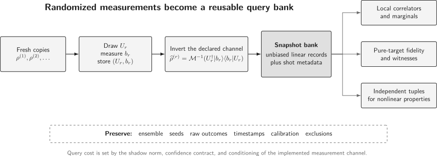
Each state copy produces a basis-and-outcome record. Inverting the declared measurement channel creates a reusable snapshot bank, but the uncertainty of each later query still depends on how well the acquisition ensemble covered that observable.

Local Pauli Shadows

The most accessible qubit protocol chooses an independent basis $P_i\in\{X,Y,Z\}$ for every qubit, measures the corresponding eigenvalue $s_i\in\{+1,-1\}$, and records $(P_i,s_i)$.

One qubit

For one qubit, the observed projector is

$$\Pi_{P,s} = \frac{I+sP}{2}.$$

Uniformly choosing $X$, $Y$, or $Z$ shrinks every Bloch-vector component by a factor of three:

$$\mathcal M(A) = \frac{A+\operatorname{Tr}(A)I}{3}.$$

Applying the inverse to an observed projector gives

$$\widehat\rho = 3\Pi_{P,s}-I = \frac{I+3sP}{2}.$$

Its trace is one, but its eigenvalues are $2$ and $-1$. A negative eigenvalue is not a reconstruction failure; it is what permits linear unbiased inversion from incomplete one-shot data.

Many qubits

For independent local choices, the measurement channel factorizes. The $n$-qubit snapshot is

$$\widehat\rho = \bigotimes_{i=1}^n \left( 3\Pi_{P_i,s_i}-I \right).$$

One should almost never construct this $2^n\times2^n$ matrix explicitly. The basis labels and outcome bits already form a compact representation from which local queries can be evaluated.

Exact Cost for a Pauli String

Let

$$W = \bigotimes_{i=1}^n W_i, \qquad W_i\in\{I,X,Y,Z\},$$

and let $S=\{i:W_i\neq I\}$ be its support, with weight $w=|S|$. For one local Pauli snapshot,

$$\widehat w = \operatorname{Tr}(W\widehat\rho) = 3^w \left( \prod_{i\in S}s_i \right) \mathbf 1 \!\left[ P_i=W_i\ \text{for all }i\in S \right].$$

The indicator is nonzero only when every randomly selected basis matches the target string on its support. This happens with probability $3^{-w}$. On matching rounds, the product of outcomes has conditional mean $\operatorname{Tr}(W\rho)$. Therefore

$$\mathbb E(\widehat w) = \operatorname{Tr}(W\rho).$$

The second moment is state independent:

$$\mathbb E(\widehat w^2) = 3^{-w}\,9^w = 3^w,$$

and hence

$$\operatorname{Var}(\widehat w) = 3^w - \operatorname{Tr}(W\rho)^2.$$

This exact result captures both the power and the limitation of local shadows. The cost does not depend on the total number of qubits, but it grows exponentially with the number of qubits touched by the observable.

For a Pauli Hamiltonian

$$H=\sum_\alpha c_\alpha W_\alpha,$$

the same snapshot estimates every covered term. The one-shot energy estimator is

$$\widehat h = \sum_\alpha c_\alpha\widehat w_\alpha.$$

Covariances between terms matter. Adding the individual variances as if all terms were measured on independent data can understate or overstate the actual energy uncertainty.

Global Clifford Shadows

At the other extreme, choose a uniformly random $n$-qubit Clifford unitary and then measure in the computational basis. For dimension $d=2^n$, the associated measurement channel is

$$\mathcal M(A) = \frac{ A+\operatorname{Tr}(A)I }{d+1},$$

so the snapshot is

$$\widehat\rho = (d+1)U^\dagger |b\rangle\langle b|U-I.$$

Although the Hilbert space is exponentially large, a Clifford $U$ and the resulting stabilizer state can be stored and manipulated with tableau methods. Stabilizer Simulation develops that representation.

For a centered observable

$$O_0 = O-\frac{\operatorname{Tr}(O)}{d}I,$$

global Clifford shadows obey a useful bound of the form

$$\|O_0\|_{\mathrm{sh}}^2 \leq 3\operatorname{Tr}(O_0^2).$$

This favors observables with small Hilbert–Schmidt norm, such as a rank-one projector onto a known pure target. It does not favor a full-weight Pauli operator, for which $\operatorname{Tr}(W^2)=d$. Global Clifford circuits also require nonlocal scrambling whose depth, noise, and compilation cost may erase their copy-complexity advantage on actual hardware.

Choosing a Measurement Ensemble

There is no universally best shadow.

Ensemble	Quantum acquisition	Natural targets	Principal cost
Independent local Pauli or single-qubit Clifford	Basis rotation and readout on each qubit	Few-body Pauli correlators, local Hamiltonians, bounded-size marginals	Variance grows as $3^w$ for a weight-$w$ Pauli
Global Clifford	Entangling Clifford randomization followed by readout	Low-rank global observables and pure-state fidelities	Circuit depth, noise, and possible exponential cost for local full-rank operators
Biased or derandomized product measurements	Target-aware local basis schedule	A known list of Pauli terms with uneven importance	Reuse becomes target dependent; coverage must remain explicit
Shallow random Clifford circuits	Tunable-depth local scrambling	Intermediate-scale observables	Reconstruction and shadow-norm evaluation can require nontrivial classical contraction
Fermionic Gaussian ensembles	Random number-preserving or Gaussian mode transformations	Fermionic reduced density matrices	Specialized controls and estimators

The decision variable is the total experiment, not copies alone. It includes state-preparation time, randomizing-gate error, readout, calibration, classical preprocessing, query cost, and the desired confidence statement.

Shadow Norm and Simultaneous Prediction

The identity component of $O$ is known exactly because $\operatorname{Tr}\rho=1$, so define the centered operator $O_0$ as above. For a fixed shadow protocol, one useful worst-case definition is

$$\|O_0\|_{\mathrm{sh}}^2 = \sup_{\sigma} \mathbb E_{\widehat\rho\sim\sigma} \left| \operatorname{Tr} \!\left( O_0\widehat\rho \right) \right|^2,$$

where the supremum runs over density operators $\sigma$. The precise norm or seminorm used in a theorem can vary with the estimator and ensemble, but its role is stable: it controls the largest single-shot second moment.

For $M$ fixed observables $O_1,\ldots,O_M$, suppose

$$B \geq \max_{1\leq j\leq M} \|(O_j)_0\|_{\mathrm{sh}}^2.$$

A median-of-means classical-shadow estimator then achieves

$$\left| \widehat o_j - \operatorname{Tr}(O_j\rho) \right| \leq\epsilon$$

for every $j$ with failure probability at most $\delta$, using

$$N = O\!\left[ \frac{B}{\epsilon^2} \log\!\left( \frac{2M}{\delta} \right) \right]$$

independent snapshots. Constants depend on the aggregation theorem and conventions.

The logarithm in $M$ comes from requiring one dataset to succeed for all queries simultaneously. It does not remove the factor $B$, the cost of implementing the ensemble, or the classical work needed to evaluate $M$ answers.

Median of means

Partition $N=KL$ snapshots into $K$ groups of size $L$. For observable $O_j$, form

$$\overline o_j^{(k)} = \frac{1}{L} \sum_{r=(k-1)L+1}^{kL} \operatorname{Tr} \!\left( O_j\widehat\rho^{(r)} \right),$$

then return

$$\widehat o_j = \operatorname{median} \left\{ \overline o_j^{(1)}, \ldots, \overline o_j^{(K)} \right\}.$$

The group mean reduces variance; the median suppresses the influence of the heavy tails created by inverse-channel weights. Typically $L$ scales as $B/\epsilon^2$ and $K$ as $\log(M/\delta)$.

This theorem presumes a finite query family fixed independently of the observed shot noise. The acquired shadow can certainly be reused for later questions, but unlimited data-dependent searching requires a holdout set, an adaptive data-analysis argument, or a new confidence statement.

Worked Example: Bell-State Fidelity

For

$$|\Phi^+\rangle = \frac{|00\rangle+|11\rangle}{\sqrt2},$$

the target projector has Pauli expansion

$$|\Phi^+\rangle\langle\Phi^+| = \frac14 \left( I\otimes I +X\otimes X -Y\otimes Y +Z\otimes Z \right).$$

Thus the fidelity with an arbitrary two-qubit preparation $\rho$ is

$$F_{\Phi^+} = \frac14 \left[ 1 +\langle X\otimes X\rangle -\langle Y\otimes Y\rangle +\langle Z\otimes Z\rangle \right].$$

One bank of local Pauli shadows estimates all three correlators. For each snapshot define $\widehat x$, $\widehat y$, and $\widehat z$ by the Pauli-string rule, then

$$\widehat F^{(r)} = \frac14 \left( 1+\widehat x^{(r)} -\widehat y^{(r)} +\widehat z^{(r)} \right)$$

is unbiased. A single value can lie below zero or above one because it is a Monte Carlo contribution, not a physical fidelity. Clipping each contribution to $[0,1]$ would generally introduce bias. Physical range constraints belong to the interpretation of the final interval, not to an undocumented nonlinear modification of the raw estimator.

This example also shows why observable structure matters. Only three weight-two strings are needed; reconstructing all fifteen two-qubit Pauli coordinates would answer a broader question at additional cost.

Many Local Marginals

For a subset $A$ of $k$ qubits,

$$\rho_A = \frac{1}{2^k} \sum_{W_A\in\mathcal P_k} \langle W_A\rangle W_A.$$

Local Pauli shadows can estimate all Pauli coordinates for every $k$-qubit subset. The number of requested correlators is at most

$$M_k \leq \binom{n}{k}4^k.$$

Since each has weight at most $k$, the simultaneous coordinate-wise sample scaling is

$$N = O\!\left[ \frac{3^k}{\epsilon^2} \left( k\log n +k +\log\frac{1}{\delta} \right) \right].$$

For fixed $k$, this grows only logarithmically with the total system size. But coordinate-wise error $\epsilon$ is not the same as trace-distance error of every $\rho_A$. Combining $4^k$ uncertain coordinates into a matrix norm requires a separate error propagation and can add substantial $k$ dependence. Reduced Density Operators owns the physical interpretation of these marginals.

Target-Aware Product Measurements

Uniformly sampling $X$, $Y$, and $Z$ is robust and reusable, but it wastes shots when the target list is strongly anisotropic. Suppose qubit $i$ chooses basis $P$ with probability $p_i(P)>0$. The local snapshot becomes

$$\widehat\rho_i = \frac12 \left[ I +\frac{s_i}{p_i(P_i)}P_i \right].$$

For a target Pauli string $W$ with support $S$, the estimator is nonzero on matching rounds and has second moment

$$\mathbb E(\widehat w^2) = \prod_{i\in S} \frac{1}{p_i(W_i)}.$$

Increasing the probability of important bases lowers their variance. Setting a needed probability to zero makes that operator direction unidentifiable.

Locally biased shadows optimize probabilities against a known Hamiltonian or observable list. Derandomized methods construct an explicit basis schedule whose coverage objective is at least as good as an associated random schedule. These methods can reduce shot counts dramatically, but the resulting dataset is less universal. The target list, term weights, scheduling algorithm, and coverage counts become part of the reported estimand.

Linear and Nonlinear Properties

The elementary snapshot identity is linear in $\rho$. It directly covers $\operatorname{Tr}(O\rho)$, including fidelity with a known pure state because

$$F(\rho,|\psi\rangle) = \langle\psi|\rho|\psi\rangle.$$

Nonlinear quantities require independent-snapshot combinations. For example, purity can be estimated without finite-sample self-pairing bias by the U-statistic

$$\widehat{\mathcal P} = \frac{1}{N(N-1)} \sum_{r\neq s} \operatorname{Tr} \!\left( \widehat\rho^{(r)} \widehat\rho^{(s)} \right).$$

Independence and unbiasedness give

$$\mathbb E \operatorname{Tr} \!\left( \widehat\rho^{(r)} \widehat\rho^{(s)} \right) = \operatorname{Tr}(\rho^2), \qquad r\neq s.$$

Higher-degree polynomial functionals use tuples of distinct snapshots. Their variance and computation can be much worse than for linear observables. Entropy estimation is additionally unstable near small eigenvalues and needs its own approximation, continuity, or structural assumptions. One should not apply the linear-observable $\log M$ theorem unchanged to purity, entropy, negativity, or mixed-state Uhlmann fidelity.

Noise Changes the Inverse

Suppose the implemented randomizing gates and detector define $\widetilde{\mathcal M}$, while software applies the ideal inverse $\mathcal M^{-1}$. Then

$$\mathbb E(\widehat\rho_{\mathrm{ideal}}) = \mathcal M^{-1} \widetilde{\mathcal M}(\rho),$$

not $\rho$. The bias in an observable is

$$\operatorname{bias}(O) = \operatorname{Tr} \!\left[ O \left( \mathcal M^{-1}\widetilde{\mathcal M} -\mathcal I \right)(\rho) \right].$$

Randomization can simplify certain noise channels, and calibration experiments can estimate correction factors. Robust-shadow protocols exploit this fact. Their guarantees still depend on assumptions such as stationary, gate-independent or suitably twirled noise, a trusted calibration preparation, and an invertible calibrated channel.

Inversion amplifies weakly observed directions. If a calibrated channel eigenvalue is small, dividing by it can remove bias while greatly increasing variance and sensitivity to calibration error. A correction should therefore report both the corrected central value and the induced sampling overhead. Measurement Tomography owns full detector reconstruction; a shadow calibration is usually a narrower model.

Drift, Leakage, and Shot Dependence

If shot $r$ prepares $\rho_r$, an otherwise ideal shadow estimator targets the average state

$$\overline\rho = \frac1N \sum_{r=1}^N \rho_r.$$

That average may be scientifically meaningful, but it is not evidence that one stationary state existed. Correlated drift also invalidates confidence formulas that treat all snapshots as independent.

Useful defenses include:

• randomizing and interleaving measurement settings in time;
• recording timestamps, calibration identifiers, leakage flags, and shot exclusions;
• forming blocks that exceed the observed correlation time;
• comparing early, middle, and late shadow estimates;
• reserving repeated settings or observables as held-out checks;
• repeating the experiment under independently prepared calibrations.

Leakage creates a separate issue: binary outcomes may no longer describe a qubit POVM. Postselecting leaked shots changes the estimand to a conditional state and must be declared.

Storage and Classical Cost

A local Pauli snapshot needs only $n$ basis labels and $n$ outcome bits, plus metadata. For a weight-$w$ Pauli query, evaluation touches only those $w$ positions. A global Clifford snapshot can be stored as a circuit seed or stabilizer tableau rather than a dense matrix.

Compact acquisition does not guarantee compact analysis:

• evaluating an explicit list of $M$ observables generally costs at least enough time to write $M$ answers;
• a dense observable may have exponentially many Pauli terms;
• nonlinear U-statistics naively require $O(N^2)$ snapshot pairs;
• uncertainty analysis over many correlated targets can dominate point estimation;
• reconstructing every local marginal can produce a large output even when the shot count is modest.

Store the primitive basis-and-outcome records whenever possible. Materializing dense snapshot matrices loses the protocol’s main computational advantage.

A Defensible Workflow

1. Define the query contract. List the target observables or function class, additive or relative precision, confidence level, subsystem, time window, and whether future exploratory queries are anticipated.
2. Choose an ensemble against the targets. Bound or estimate the relevant shadow norms and include randomizing-circuit depth, noise, calibration, and postprocessing in the comparison.
3. Verify coverage. Check invertibility on every target direction. For product measurements, audit basis probabilities and realized match counts.
4. Calibrate the implemented measurement channel. Record the calibration states, assumptions, uncertainty, condition numbers, and validity interval.
5. Acquire randomized, timestamped shots. Preserve unitary or basis seeds, outcomes, shot ordering, heralds, leakage information, and exclusions.
6. Construct snapshots transparently. Version the inverse map and test it on simulated states and calibration data with known expectations.
7. Aggregate with the declared estimator. Keep mean, median-of-means, clipping, shrinkage, and physical projection distinct; they have different bias and uncertainty.
8. Validate beyond the queried list. Use held-out observables, repeated blocks, direct-measurement comparisons, and residual checks for drift or model failure.
9. Report the full resource ledger. Include state copies, circuit depth, two-qubit gates, discarded shots, calibration shots, classical runtime, memory, and query count.
10. Publish reproducible artifacts. Reproducible Notebooks explains the required environment, provenance, and clean-execution record.

Minimum Reporting Record

A reusable shadow dataset should identify:

• the physical state-preparation circuit and its parameter version;
• qubit or mode ordering and all basis conventions;
• the random-unitary ensemble and sampling distribution;
• random seeds or the complete per-shot measurement schedule;
• raw outcomes, timestamps, heralds, and leakage treatment;
• calibration circuits, fitted channel, assumptions, and uncertainty;
• the exact inverse or estimator implementation;
• target observables and whether they were prespecified or exploratory;
• aggregation method, group partition, confidence procedure, and multiple-query correction;
• held-out tests, exclusions, software versions, and hardware calibration identifiers.

Without this record, the phrase “classical shadow” does not specify a reproducible statistical experiment.

Common Mistakes

“The number of measurements is independent of system size”

Only under a target family whose shadow norm remains controlled. Local Pauli shadows pay $3^w$ for Pauli weight $w$; global Clifford shadows pay according to a different operator geometry.

Treating a snapshot as a density matrix

Individual snapshots can have negative eigenvalues and large operator norm. Projecting each one to the positive cone changes the estimator and usually introduces bias.

Quoting only the logarithm in the number of observables

The complete scaling includes the shadow norm, $\epsilon^{-2}$, confidence, implementation cost, and classical query cost.

Ignoring target selection

A simultaneous guarantee covers a declared finite family. Searching the same data for whichever observable looks most anomalous creates selection bias.

Using an ideal inverse on noisy data

The result estimates $\mathcal M^{-1}\widetilde{\mathcal M}(\rho)$ unless the implemented channel is calibrated or otherwise justified.

Assuming randomization removes noise

Twirling can simplify noise under assumptions; it does not certify those assumptions or erase drift, leakage, and gate dependence.

Applying a linear theorem to nonlinear quantities

Purity, entropy, and mixed-state fidelity require distinct estimators and error analyses.

Comparing ensembles by shots alone

A deep global randomizer and a local basis change are not equivalent experimental resources.

Forgetting covariance

Many observables evaluated on the same snapshots are statistically correlated. That correlation matters for Hamiltonian sums, witnesses, and fitted models.

Calling targeted prediction full tomography

A shadow may answer a large query family accurately while remaining poor in trace distance as an approximation to the entire state.

Further Connections

• State Tomography explains what is gained and paid for when the goal changes from selected properties to a physical full-state estimate.
• Certification of Entanglement uses shadow estimates for simultaneous witness queries while retaining the separability bound, ensemble calibration, and selection correction.
• Randomized Benchmarking uses random gate sequences to estimate an ensemble decay; its randomization, estimand, and statistical hierarchy differ from randomized-measurement shadows.
• Why Benchmarking Is Hard places shadow-derived observables inside a broader validation contract.
• Density Operators for Quantum Information develops the state representation whose linear functionals are being estimated.
• Pauli Matrices supplies the operator basis used by local qubit shadows.
• Fidelity distinguishes the pure-target linear overlap from nonlinear mixed-state fidelity.
• Metrics for Quantum Hardware discusses what a measured observable or fidelity does and does not establish about a processor.

References

• Scott Aaronson, “Shadow Tomography of Quantum States”, Proceedings of STOC 2018, 2018 — original shadow-tomography problem and polylogarithmic copy bound.
• Hsin-Yuan Huang, Richard Kueng, and John Preskill, “Predicting Many Properties of a Quantum System from Very Few Measurements”, Nature Physics 16, 1050–1057 (2020) — classical-shadow protocol, shadow norms, and simultaneous prediction.
• Marco Paini and Amir Kalev, “An Approximate Description of Quantum States”, Quantum 3, 197 (2019) — independent development of reusable randomized local-measurement estimators.
• Hsin-Yuan Huang, Richard Kueng, and John Preskill, “Efficient Estimation of Pauli Observables by Derandomization”, Physical Review Letters 127, 030503 (2021) — target-aware deterministic measurement schedules.
• Charles Hadfield, Sergey Bravyi, Rudy Raymond, and Antonio Mezzacapo, “Measurements of Quantum Hamiltonians with Locally-Biased Classical Shadows”, Communications in Mathematical Physics 391, 951–967 (2022) — biased product ensembles for Hamiltonian estimation.
• Senrui Chen, Wenjun Yu, Pei Zeng, and Steven T. Flammia, “Robust Shadow Estimation”, PRX Quantum 2, 030348 (2021) — calibration-based mitigation under stated noise assumptions.
• Dax Enshan Koh and Sabee Grewal, “Classical Shadows with Noise”, Quantum 6, 776 (2022) — noisy measurement channels, unbiased corrections, and noise-dependent sample bounds.
• G. I. Struchalin, Ya. A. Zagorovskii, E. V. Kovlakov, S. S. Straupe, and S. P. Kulik, “Experimental Estimation of Quantum State Properties from Classical Shadows”, PRX Quantum 2, 010307 (2021) — experimental high-dimensional property estimation and estimator-bias comparisons.
• Hong-Ye Hu, Soonwon Choi, and Yi-Zhuang You, “Classical Shadow Tomography with Locally Scrambled Quantum Dynamics”, Physical Review Research 5, 023027 (2023) — finite-depth local randomization and entanglement-feature inversion.
• Christian Bertoni, Jonas Haferkamp, Marcel Hinsche, Marios Ioannou, Jens Eisert, and Hakop Pashayan, “Shallow Shadows: Expectation Estimation Using Low-Depth Random Clifford Circuits”, Physical Review Letters 133, 020602 (2024) — depth-tunable shadows and computable performance bounds.
• Andrew Zhao, Nicholas C. Rubin, and Akimasa Miyake, “Fermionic Partial Tomography via Classical Shadows”, Physical Review Letters 127, 110504 (2021) — symmetry-compatible shadows for fermionic reduced density matrices.
• Daniel Grier, Hakop Pashayan, and Luke Schaeffer, “Sample-Optimal Classical Shadows for Pure States”, 2022 — refined upper and lower bounds showing dependence on state and measurement resources.
• Andreas Elben, Steven T. Flammia, Hsin-Yuan Huang, Richard Kueng, John Preskill, Benoît Vermersch, and Peter Zoller, “The Randomized Measurement Toolbox”, Nature Reviews Physics 5, 9–24 (2023) — review connecting classical shadows, randomized measurements, experiments, and noise.
• Ryan Levy, Di Luo, and Bryan K. Clark, “Classical Shadows for Quantum Process Tomography on Near-Term Quantum Computers”, Physical Review Research 6, 013029 (2024) — extension from state properties to selected channel properties.
• Simon Becker, Nilanjana Datta, Ludovico Lami, and Cambyse Rouzé, “Classical Shadow Tomography for Continuous Variables Quantum Systems”, IEEE Transactions on Information Theory 70, 3427–3452 (2024) — energy-constrained continuous-variable shadows.

Exercises

1. Unbiasedness and invisible directions

Let $\mathcal M$ be invertible only on an operator subspace $\mathcal S$. Show that the snapshot estimator is unbiased for every observable $O\in\mathcal S$, provided the inverse is interpreted on $\mathcal S$. Explain why no estimator built from the same data can identify a direction in $\ker\mathcal M$ without an additional assumption.

Solution

Let $\mathcal M_{\mathcal S}^{-1}$ denote the inverse restricted to $\mathcal S$. For the component $\rho_{\mathcal S}$ visible to the measurement,

$$\mathbb E(\widehat\rho_{\mathcal S}) = \mathcal M_{\mathcal S}^{-1} \mathcal M(\rho) = \rho_{\mathcal S}.$$

If $O\in\mathcal S$, its expectation depends only on this visible component, so

$$\mathbb E \operatorname{Tr} \!\left( O\widehat\rho_{\mathcal S} \right) = \operatorname{Tr}(O\rho).$$

Now let $A\in\ker\mathcal M$. States $\rho$ and $\rho+tA$, whenever both are physical, produce the same measurement statistics because

$$\mathcal M(\rho+tA) = \mathcal M(\rho).$$

No data-only estimator can distinguish them. Identifying $A$ requires another measurement, a structural prior, or a model constraint that rules out one of the states.

2. Derive the one-qubit Pauli snapshot

Write

$$\rho = \frac12 \left( I+r_xX+r_yY+r_zZ \right).$$

Average the post-measurement rotated-back projector over uniformly random $X$, $Y$, and $Z$ bases. Derive $\mathcal M(\rho)$ and verify that $3\Pi_{P,s}-I$ is the inverse-channel snapshot.

Solution

For a fixed basis $P$, averaging the observed projector over outcomes dephases $\rho$ in that basis:

$$\sum_s \operatorname{Tr}(\Pi_{P,s}\rho)\, \Pi_{P,s} = \frac12 \left( I+r_P P \right).$$

Averaging over the three bases gives

$$\begin{aligned} \mathcal M(\rho) &= \frac13 \sum_{P=X,Y,Z} \frac12 \left( I+r_P P \right) \\ &= \frac12 \left[ I+\frac13 \left( r_xX+r_yY+r_zZ \right) \right] \\ &= \frac{\rho+I}{3}. \end{aligned}$$

More generally,

$$\mathcal M(A) = \frac{A+\operatorname{Tr}(A)I}{3}.$$

Because $\operatorname{Tr}\Pi_{P,s}=1$,

$$\mathcal M^{-1}(\Pi_{P,s}) = 3\Pi_{P,s}-I.$$

Its ensemble average is $\rho$, as required.

3. Weight controls variance

For a weight-$w$ Pauli string $W$, derive the local-shadow estimator and show

$$\operatorname{Var}(\widehat w) = 3^w-\langle W\rangle^2.$$

What changes if $w$ increases while the total number of qubits remains fixed?

Solution

Every target basis must match, which occurs with probability $3^{-w}$. The estimator is zero otherwise. On a match it equals

$$3^w\prod_{i\in S}s_i.$$

The conditional mean of the outcome product is $\langle W\rangle$, so the unconditional mean is $\langle W\rangle$. Squaring removes all signs:

$$\mathbb E(\widehat w^2) = 3^{-w}(3^w)^2 = 3^w.$$

Subtracting the squared mean gives the stated variance. Increasing $w$ by one multiplies the leading second moment by three, regardless of how many idle qubits lie outside the support. The difficulty is observable weight, not total register size by itself.

4. Bell fidelity from one dataset

For an ideal $|\Phi^+\rangle$ preparation, find the expectations of $X\otimes X$, $Y\otimes Y$, and $Z\otimes Z$. Insert them into the shadow fidelity estimator. Explain why an individual Monte Carlo contribution need not lie in $[0,1]$.

Solution

The Bell state is stabilized by $X\otimes X$ and $Z\otimes Z$, while $Y\otimes Y=-(X\otimes X)(Z\otimes Z)$. Hence

$$\langle X\otimes X\rangle=1, \qquad \langle Y\otimes Y\rangle=-1, \qquad \langle Z\otimes Z\rangle=1.$$

Therefore

$$F_{\Phi^+} = \frac14 \left[ 1+1-(-1)+1 \right] = 1.$$

A single weight-two Pauli estimator is either zero or $\pm9$. The corresponding single-shot linear combination can therefore lie far outside $[0,1]$. Only its expectation equals a physical fidelity. Range projection is nonlinear and changes the estimator’s bias.

5. Scaling for all bounded-size correlators

Estimate the number $M_k$ of Pauli correlators needed to describe every $k$-qubit marginal of an $n$-qubit state. Use the local-Pauli shadow bound to obtain the dependence of the required snapshots on $n$, $k$, $\epsilon$, and $\delta$ for simultaneous coordinate-wise accuracy.

Solution

There are $\binom nk$ subsets of size $k$ and at most $4^k$ Pauli strings per subset, so

$$M_k\leq\binom nk4^k.$$

Every requested string has weight at most $k$, so $B\leq3^k$. Substituting into the simultaneous-prediction bound gives

$$N = O\!\left[ \frac{3^k}{\epsilon^2} \log\!\left( \frac{2\binom nk4^k}{\delta} \right) \right].$$

Using $\log\binom nk\leq k\log(en/k)$,

$$N = O\!\left[ \frac{3^k}{\epsilon^2} \left( k\log\frac{en}{k} +k +\log\frac1\delta \right) \right].$$

This controls each Pauli coordinate. A matrix-norm guarantee for every marginal requires propagating the coordinate errors and is stronger.

6. Biased basis sampling

For one target string $W$ and independent basis probabilities $p_i(P)$, show that the second moment is

$$\prod_{i\in S}p_i(W_i)^{-1}.$$

Why is choosing $p_i(W_i)=1$ not a universal improvement?

Solution

The target bases match with probability

$$q_W = \prod_{i\in S}p_i(W_i).$$

On a match, the inverse-probability estimator has magnitude $q_W^{-1}$. Therefore

$$\mathbb E(\widehat w^2) = q_W q_W^{-2} = \prod_{i\in S}p_i(W_i)^{-1}.$$

Setting each needed probability to one minimizes variance for this one string. It assigns zero probability to incompatible bases, however, making other Pauli directions invisible. It is optimal only for the narrow query contract in which those other directions are irrelevant.

7. Symmetric readout flips

In a local Pauli experiment, suppose the recorded eigenvalue is flipped with known probability $q<1/2$, independently of the state and chosen basis. Show the bias of the ideal estimator for a target containing one measured Pauli factor. Give an unbiased correction and its variance-amplification factor.

Solution

If $s'$ is the recorded value, then

$$\mathbb E(s'|s) = (1-q)s+q(-s) = (1-2q)s.$$

Every affected Pauli factor therefore multiplies the target expectation by $1-2q$. For one affected factor,

$$\mathbb E(\widehat w_{\mathrm{ideal}}) = (1-2q)\langle W\rangle.$$

An unbiased correction is

$$\widehat w_{\mathrm{corr}} = \frac{\widehat w_{\mathrm{ideal}}}{1-2q}.$$

Its second moment, and hence its leading variance scale, is amplified by

$$\frac{1}{(1-2q)^2}.$$

Calibration uncertainty in $q$ adds another contribution not included in this conditional calculation.

8. Unbiased purity

Show that the U-statistic

$$\widehat{\mathcal P} = \frac{1}{N(N-1)} \sum_{r\neq s} \operatorname{Tr} \!\left( \widehat\rho^{(r)} \widehat\rho^{(s)} \right)$$

is unbiased for $\operatorname{Tr}(\rho^2)$. Why does including terms with $r=s$ generally introduce a finite-sample bias?

Solution

For $r\neq s$, the snapshots are independent. Thus

$$\begin{aligned} \mathbb E \operatorname{Tr} \!\left( \widehat\rho^{(r)} \widehat\rho^{(s)} \right) &= \operatorname{Tr} \!\left[ \mathbb E(\widehat\rho^{(r)}) \mathbb E(\widehat\rho^{(s)}) \right] \\ &= \operatorname{Tr}(\rho^2). \end{aligned}$$

Every ordered pair has the same expectation, so their average is unbiased. For a self-pair,

$$\mathbb E \operatorname{Tr} \!\left[ (\widehat\rho^{(r)})^2 \right]$$

depends on the snapshot second moment and is generally not $\operatorname{Tr}(\rho^2)$. Including the $N$ self-pairs therefore adds a bias of order $1/N$ unless it is explicitly corrected.