Cycle Benchmarking

Short Definition

Cycle benchmarking (CB) estimates the process fidelity of an implemented processor cycle: a fixed, scheduled layer of simultaneous gates, idles, frame changes, and spectator activity. The standard protocol prepares eigenstates of sampled Pauli observables, repeats a target Clifford cycle while inserting random Pauli cycles, and extracts decay rates from sign-corrected Pauli measurements.

The randomization tailors the effective error toward a Pauli channel. Repeating the dressed cycle amplifies its Pauli-fidelity losses while fixed state-preparation-and-measurement effects enter primarily through decay amplitudes. Averaging suitable decay rates over sampled Paulis gives a scalable estimate of the dressed cycle’s process fidelity.

That short description contains three qualifications that should never be dropped:

• the canonical estimand is the dressed cycle, including the implemented randomizing layer;
• a decay may identify a product of Pauli fidelities around an orbit, not each fidelity separately;
• SPAM robustness and simple exponential behavior require stability, Markovianity, a valid randomization model, and a controlled computational subspace.

This page owns cycle-level estimands, the Pauli-randomized protocol, orbit decays, statistical design, learnability, and interpretation. Randomized Benchmarking owns reference and interleaved group RB. Process Tomography owns full channel reconstruction, and Metrics for Quantum Hardware owns comparisons among hardware metrics.

Why the Cycle Is the Unit

A cycle is not merely a set of gate names. It is a set of instructions with a declared timing schedule on a declared register. A useful cycle record includes

$$\mathfrak C = (\text{operations},\text{supports},\text{timing}, \text{idles},\text{frames},\text{spectators}).$$

Two schedules implementing the same ideal unitary can therefore be different cycles. Moving a pulse, changing an echo, filling an idle, enabling a neighboring gate, or replacing a physical phase pulse by a virtual frame update can change the physical error channel.

This is exactly why cycle-level characterization is useful. A two-qubit gate tested alone does not reveal all errors present when several couplers and single-qubit drives operate in parallel. The complete cycle can expose crosstalk, drive collisions, spectator phases, correlated errors, and idle dephasing in their operational context.

The contrast with nearby methods is one of estimand rather than quality:

Method	Primary estimand	Main strength	Main boundary
process tomography	declared channel in a trusted SPAM model	detailed reconstruction	exponential parameter count and SPAM composition
reference RB	average over a sampled gate group and compiler	compact SPAM-robust decay	coarse for large compiled Cliffords
cycle benchmarking	one scheduled, Pauli-dressed cycle	parallel context and scalable fidelity	partial Pauli information under a tailoring model

CB does not make component benchmarking obsolete. It answers a different question: how accurately does this whole scheduled layer execute when used in this context?

Process Fidelity in a Pauli Basis

Consider $n$ qubits with Hilbert-space dimension

$$d=2^n.$$

Let $\mathcal G$ denote the ideal unitary channel of the target cycle and $\widetilde{\mathcal G}$ its implementation. With the convention

$$\Lambda = \mathcal G^\dagger \circ \widetilde{\mathcal G},$$

$\Lambda$ is the error channel relative to the ideal cycle. For an $n$-qubit Pauli $P$, define the Pauli fidelity

$$f_P(\Lambda) = \frac{1}{d} \operatorname{Tr} \!\left[ P\Lambda(P) \right].$$

Equivalently, without introducing $\Lambda$,

$$f_P = \frac{1}{d} \operatorname{Tr} \!\left[ \mathcal G(P) \widetilde{\mathcal G}(P) \right].$$

The Paulis form an orthogonal operator basis,

$$\operatorname{Tr}(PQ) = d\,\delta_{P,Q},$$

so the process fidelity, also called the entanglement fidelity relative to the ideal cycle, is

$$F_{\mathrm e}(\Lambda) = \frac{1}{d^2} \sum_{P\in\mathbb P_n} f_P(\Lambda).$$

For a trace-preserving channel, $f_I=1$. If only nonidentity Paulis are sampled uniformly, this known identity contribution should be restored explicitly. Writing

$$\overline f_{\ne I} = \frac{1}{d^2-1} \sum_{P\ne I} f_P,$$

gives

$$F_{\mathrm e} = \frac{1+(d^2-1)\overline f_{\ne I}}{d^2}.$$

The average gate fidelity obeys

$$F_{\mathrm{avg}} = \frac{dF_{\mathrm e}+1}{d+1}.$$

Consequently, process infidelity $e_{\mathrm e}=1-F_{\mathrm e}$ and average gate infidelity $r=1-F_{\mathrm{avg}}$ differ by

$$e_{\mathrm e} = \frac{d+1}{d}\,r.$$

A report must name which convention it uses. Calling both quantities “cycle error” without the dimensional conversion creates avoidable disagreement.

Pauli Channels and Error Probabilities

A Pauli channel has the form

$$\Lambda_{\mathrm P}(\rho) = \sum_{Q\in\mathbb P_n} \mu_Q Q\rho Q, \qquad \mu_Q\ge 0, \qquad \sum_Q\mu_Q=1.$$

Every Pauli is an eigenoperator of this channel:

$$\Lambda_{\mathrm P}(P) = f_P P.$$

Let $\chi(P,Q)$ be $+1$ when $P$ and $Q$ commute and $-1$ when they anticommute. Then

$$f_P = \sum_Q \mu_Q\chi(P,Q).$$

The inverse Walsh–Hadamard relation is

$$\mu_Q = \frac{1}{d^2} \sum_P \chi(P,Q)f_P.$$

In particular,

$$\mu_I = \frac{1}{d^2} \sum_P f_P = F_{\mathrm e}.$$

Thus, for a Pauli channel, the process infidelity is the total probability of a nonidentity Pauli error:

$$1-F_{\mathrm e} = \sum_{Q\ne I}\mu_Q.$$

This interpretation is powerful after noise tailoring. It is not a license to claim that an arbitrary coherent or non-Markovian physical process literally chooses a Pauli error independently on every cycle. Pauli Channels develops the channel representation itself.

The Dressed-Cycle Estimand

Let $\mathcal R$ be an ideal Pauli cycle and $\widetilde{\mathcal{G}\mathcal R}$ the physical implementation of the target cycle dressed by that Pauli cycle. Its relative error channel is

$$\Lambda_R = (\mathcal G\mathcal R)^\dagger \circ \widetilde{\mathcal{G}\mathcal R}.$$

The central CB estimand is the average dressed-cycle process fidelity

$$F_{\mathrm{RC}} = \frac{1}{d^2} \sum_{R\in\mathbb P_n} F_{\mathrm e}(\Lambda_R).$$

This object includes the way Pauli gates are realized. They may be physical pulses, virtual frame updates, or corrections compiled into adjacent single-qubit operations. Those choices alter the implementation and belong in the result.

The distinction between dressed and bare cycles matters operationally. If a randomized-compiled workload uses the same dressing convention, the dressed cycle is directly relevant to that workload. If an undressed workload is run, coherent errors may add or cancel differently, and the CB number need not predict its performance.

How Pauli Randomization Creates a Decay

For a fixed error channel $\Lambda$, its Pauli twirl is

$$\Lambda^{\mathbb P} = \frac{1}{d^2} \sum_{R\in\mathbb P_n} \mathcal R^\dagger \circ \Lambda \circ \mathcal R.$$

In the Pauli-transfer representation, this averaging removes off-diagonal terms and retains the diagonal Pauli fidelities. Randomized compiling places the twirling operations and their corrections into neighboring easy cycles so that the ideal computation is unchanged while the averaged error is tailored.

For a Clifford target cycle, conjugation permutes Pauli operators up to sign:

$$\mathcal G(P) = s_P\,\pi(P), \qquad s_P\in\{+1,-1\}.$$

Suppose the tailored error is stationary and Pauli diagonal. Starting with $P$, the ideal cycle moves the measured Pauli through the orbit

$$P,\quad \pi(P),\quad \pi^2(P),\quad \ldots$$

and each step contributes the corresponding Pauli fidelity. The sequence-averaged signal has the baseline form

$$S_P(m) = A_P \prod_{j=0}^{m-1} f_{\pi^j(P)}.$$

Here $A_P$ contains fixed preparation, measurement, and edge effects after the protocol’s sign projection. If the orbit has length $\ell$ and $m=t\ell$, define

$$g_{\mathcal O} = \left( \prod_{j=0}^{\ell-1} f_{\pi^j(P)} \right)^{1/\ell}.$$

Then

$$S_P(t\ell) = A_P g_{\mathcal O}^{\,t\ell}.$$

The fitted decay therefore identifies an orbit geometric mean. It identifies a single $f_P$ only when $P$ is fixed by the ideal cycle or when additional information breaks the orbit product into its factors.

Example: a controlled-Z orbit

For an ideal controlled-$Z$ cycle,

$$XI \longmapsto XZ \longmapsto XI.$$

A compatible CB decay determines

$$g_{\{XI,XZ\}} = \sqrt{f_{XI}f_{XZ}}.$$

It does not separately identify $f_{XI}$ and $f_{XZ}$. By contrast, $ZI$, $IZ$, and $ZZ$ are fixed under controlled-$Z$ conjugation, so their corresponding decays can identify individual Pauli fidelities under the baseline model.

The Standard Protocol

A defensible implementation separates ideal circuit construction, physical compilation, sampling, and statistical inference.

1. Freeze the cycle contract. Record the qubits, active operations, idles, timing, pulse and frame implementations, spectators, compiler version, and calibration snapshot.
2. Choose test Paulis. Sample $K$ nonidentity Paulis from a declared distribution. Product-Pauli eigenstates permit local preparation and measurement, but their basis operations are still noisy.
3. Choose compatible lengths. Select lengths for which the ideal Clifford action gives the same effective preparation and measurement contract. A simple choice uses $m_1$ and $m_2$ satisfying

$$\mathcal G^{m_1} = \mathcal G^{m_2} = \mathcal I.$$

4. Generate random circuits. For each $P$, length $m$, and random-sequence index $l$, sample Pauli cycles and construct

$$\begin{aligned} \mathcal C_{m,l} ={}& \mathcal R_{m,l}\mathcal G \mathcal R_{m-1,l}\mathcal G \cdots \\ &\cdots \mathcal R_{1,l}\mathcal G \mathcal R_{0,l}. \end{aligned}$$

5. Compute the ideal sign. Stabilizer propagation gives the Pauli measured at the output and the sign induced by the sampled randomizers. Applying this sign in post-processing is part of the protocol, not an optional cosmetic correction.
6. Prepare, execute, and measure. Prepare a $+1$ eigenstate of $P$, run the compiled circuit, measure the predicted output Pauli, and retain raw outcomes rather than only an averaged expectation.
7. Estimate each decay. Average over shots within a sequence and over independent random sequences at fixed $(P,m)$.
8. Average over Paulis. Convert the sampled nonidentity mean to process fidelity using the known identity contribution, and report uncertainty from every sampling level.

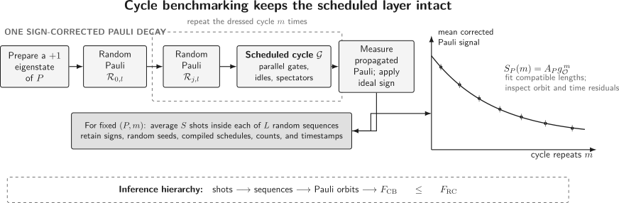
Cycle benchmarking preserves the scheduled target cycle while random Pauli layers tailor its effective noise. Sign-corrected Pauli expectations are aggregated first over shots and random sequences, then over sampled Pauli orbits to estimate a dressed-cycle process fidelity.

Unlike reference RB, this circuit need not end with one large group inversion. The final Pauli correction and classical sign account for the randomization, while Clifford propagation keeps the ideal output efficiently computable.

Two-Length and Multi-Length Estimation

Let

$$\overline S_P(m) = \frac{1}{L} \sum_{l=1}^{L} \widehat S_{P,m,l}$$

be the mean sign-corrected signal over $L$ random sequences. If the same amplitude $A_P$ applies at two compatible lengths, the decay estimate is

$$\widehat g_P = \left[ \frac{\overline S_P(m_2)} {\overline S_P(m_1)} \right]^{1/(m_2-m_1)}.$$

The amplitude cancels. For Paulis sampled uniformly from the nonidentity set, the process-fidelity estimator is

$$\widehat F_{\mathrm{CB}} = \frac{ 1+(d^2-1) K^{-1}\sum_{k=1}^{K}\widehat g_{P_k} }{d^2}.$$

At the population level, standard CB gives a lower bound on the dressed process fidelity and differs from it only at second order in the total error:

$$F_{\mathrm{CB}} \le F_{\mathrm{RC}},$$ $$F_{\mathrm{RC}}-F_{\mathrm{CB}} = \mathcal O \!\left[ (1-F_{\mathrm{RC}})^2 \right].$$

The lower-bound statement concerns ideal population quantities under the protocol assumptions. A finite-data point estimate can fluctuate above the true fidelity, so it still needs a confidence or credible interval.

Two lengths can be economical, but three or more compatible lengths are more diagnostic. They permit a direct fit

$$S_P(m) = A_P g_P^m$$

and expose curvature, length-dependent amplitudes, leakage modes, drift, or a poor orbit model. A two-point ratio cannot test its own exponential assumption.

Worked Two-Qubit Example

Suppose a two-qubit cycle is tested at $m_1=4$ and $m_2=12$. For one Pauli orbit, the sequence-averaged corrected signals are

$$\overline S_P(4)=0.842, \qquad \overline S_P(12)=0.790.$$

The orbit decay is

$$\begin{aligned} \widehat g_P &= \left( \frac{0.790}{0.842} \right)^{1/8} \\ &\simeq 0.9921. \end{aligned}$$

This number is independent of an unknown constant amplitude only if the same effective SPAM map applies at both lengths.

Now suppose the mean decay over the sampled nonidentity Paulis is

$$\overline g_{\ne I}=0.990.$$

For $d=4$,

$$\begin{aligned} \widehat F_{\mathrm e} &= \frac{1+15(0.990)}{16} \\ &= 0.990625. \end{aligned}$$

The process infidelity is $0.009375$. The corresponding average gate infidelity is

$$\begin{aligned} \widehat r &= \frac{d}{d+1} (1-\widehat F_{\mathrm e}) \\ &= \frac{4}{5}(0.009375) \\ &= 0.0075. \end{aligned}$$

Reporting “cycle error $=0.75\%$” would therefore mean average gate infidelity, whereas “process infidelity $=0.9375\%$” uses the entanglement-fidelity convention.

Paulis, Sequences, Shots, and Time Blocks

CB has at least four distinct sampling levels:

• $K$ sampled test Paulis;
• $L_{P,m}$ random circuits for each Pauli and length;
• $S_{P,m,l}$ shots for each random circuit;
• time blocks, calibrations, or experimental batches.

Let $z_{P,m,l,s}\in\{-1,+1\}$ be a sign-corrected shot and

$$\widehat S_{P,m,l} = \frac{1}{S} \sum_{s=1}^{S} z_{P,m,l,s}.$$

If the true sequence signal is $S_{P,m,l}$, then a useful variance decomposition is

$$\begin{aligned} \operatorname{Var} \!\left[ \overline S_P(m) \right] ={}& \frac{\sigma_{\mathrm{seq}}^2}{L} \\ &+ \frac{1}{L} \mathbb E_l \!\left[ \frac{1-S_{P,m,l}^2}{S} \right]. \end{aligned}$$

The first term is variation among random circuits. The second is finite-shot noise within a circuit. Increasing shots cannot remove the first term. Likewise, increasing sequences for one Pauli cannot remove variation across the sampled Pauli population.

An uncertainty analysis should preserve this hierarchy. Suitable approaches include a hierarchical likelihood, a cluster bootstrap over random sequences, and a block bootstrap over chronological batches. Bootstrapping individual shots as if all shots were independent usually understates uncertainty.

Allocating an experimental budget

Early pilot data should estimate the relative sizes of Pauli, sequence, shot, and drift variation. Then:

• add shots when binomial noise dominates;
• add independent random circuits when sequence variation dominates;
• add sampled Paulis when the fidelity estimate changes across Pauli directions;
• interleave time blocks and recalibrations when drift dominates.

The optimal allocation is device and cycle dependent. A fixed recipe such as “30 circuits and 100 shots” is a starting point, not a statistical theorem.

What SPAM Robustness Means

Under the baseline model, fixed preparation and measurement errors multiply the signal by $A_P$:

$$S_P(m)=A_P g_P^m.$$

Ratios or fitted decay rates can then remove that fixed amplitude. This is the precise sense in which CB is SPAM robust.

It does not mean:

• preparation and measurement are ideal;
• SPAM errors have no effect on variance;
• the basis-change gates are outside the implementation;
• readout drift between lengths cancels;
• leakage during preparation or measurement is harmless;
• a different output observable may be used at each length without analysis.

Compatible lengths are valuable because they can make the ideal output Pauli and its measurement procedure identical. Randomizing the order of lengths and repeating them across time blocks helps distinguish a physical decay from a moving SPAM amplitude.

Learnability and Gauge Freedom

Orbit products are not merely a fitting inconvenience. They express a fundamental learnability boundary.

For a Clifford gate set with Pauli-diagonal noise, one can construct a pattern transfer graph. Its vertices encode Pauli support patterns, and each directed edge carries a log Pauli fidelity. A CB experiment that returns to its starting pattern measures a sum around a graph cycle:

$$\log g_{\mathcal O}^{\ell} = \sum_{P\in\mathcal O} \log f_P.$$

The learnable linear combinations form the graph’s cycle space. Complementary cut-space directions are gauge degrees of freedom: changing them can be absorbed into SPAM descriptions without changing observable circuit probabilities. Consequently, physical constraints may bound an unlearnable direction, but data do not identify it simply because an optimizer returns one number.

This distinction becomes essential when moving from total process fidelity to a detailed Pauli error model. The latter needs additional cycles, assumptions such as locality or sparsity, trusted operations, or other experiments.

Dressed Fidelity Is Not Bare-Cycle Fidelity

A common extension compares a target dressed-cycle fidelity $F_{\mathrm{tgt}}$ with a reference dressing fidelity $F_{\mathrm{ref}}$ and forms a ratio,

$$\widehat F_{\mathrm{bare}} \approx \frac{F_{\mathrm{tgt}}} {F_{\mathrm{ref}}}.$$

This resembles interleaved RB. The ratio can be useful when the reference errors are weak, suitably independent, and compose benignly with the target error. In general, however, fidelity is not multiplicative:

$$F_{\mathrm e} (\Lambda_2\circ\Lambda_1) \ne F_{\mathrm e}(\Lambda_2) F_{\mathrm e}(\Lambda_1).$$

Coherent errors can reinforce or cancel, and gate-dependent randomizer errors can correlate with the target. The inferred bare-cycle fidelity can therefore have systematic uncertainty on the scale of the total error. It should be labeled as an inference under stated assumptions, not as a direct CB output.

Assumptions and Failure Modes

Stationarity and Markovianity

The simplest derivation assigns the same effective channel to every repeated cycle. Drift makes the channel depend on clock time; memory makes it depend on earlier randomizers or outcomes. Either can produce length-dependent rates, overdispersion, or apparent multi-exponential behavior.

Estimate the fidelity using more than one pair of lengths. Under the stationary model, compatible pairs should agree within uncertainty. Preserve acquisition order so that a time-resolved residual analysis remains possible.

Randomizer dependence

Pauli twirling is exact for an abstract fixed channel conjugated by ideal Paulis. Physical easy cycles are noisy and may have gate-dependent errors. Randomized compiling gives useful guarantees under stated assumptions, but the effective dressed-cycle interpretation still includes the compilation rule and the randomizer implementation.

Compare virtual and physical randomization where possible, inspect randomizer-conditioned residuals, and report whether corrections were absorbed into neighboring pulses.

Leakage and loss

Leakage leaves the computational Pauli space. A leaked population can add slow modes, offsets, or apparent decay floors:

$$S_P(m) \approx A_P g_P^m + C_P \ell_P^m + B_P.$$

A good single-exponential fit over a short range does not prove leakage is absent. Pair CB with survival measurements, leakage-sensitive readout, or a declared enlarged-space model. Noise in Quantum Information owns the physical error taxonomy.

Non-Clifford target cycles

The simple protocol uses efficient Pauli propagation under a Clifford cycle. General non-Clifford cycles do not permute Paulis, so the observable can spread into a sum of operators and the single-orbit picture fails. Extensions based on randomized compiling or broader representation-theoretic protocols exist, but their estimands and post-processing must be specified separately.

Coherent error and undressed workloads

Pauli randomization converts coherent contributions into an effective stochastic description in the averaged randomized circuit. This is useful for randomized-compiled workloads. It does not imply that the undressed cycle’s worst-case error is small, nor that coherent accumulation in a fixed circuit has been measured.

Scaling: What Is and Is Not Efficient

There are $d^2=4^n$ Pauli fidelities, so learning every diagonal element without structure remains exponential. CB avoids this cost when the goal is one average fidelity to fixed additive precision: one samples Pauli directions rather than enumerating all of them. Under the baseline assumptions, the number of sampled Paulis required for that average need not grow with $n$.

Several costs still grow:

• each Pauli string acts across the declared register;
• preparation and measurement require local basis operations and readout;
• compiled circuits grow with sequence length;
• correlated readout and leakage become harder to control;
• estimating rare or high-weight error probabilities needs more information than estimating one average.

“Scalable” therefore describes a fixed-precision partial characterization. It does not mean full process tomography in disguise.

Beyond a Single Fidelity

Later protocols reuse CB-structured circuits for more detailed diagnostics.

Cycle error reconstruction estimates selected marginal Pauli error distributions of effective dressed cycles, commonly using locality or sparsity to remain scalable. Its multiplicative-precision goals and reconstruction assumptions go beyond standard total-fidelity CB.

Pauli-noise learnability analyses characterize exactly which combinations of Pauli fidelities are observable in the presence of SPAM gauge freedom. They show why adding related cycles can enlarge the learnable cycle space.

Multi-layer cycle benchmarking jointly analyzes several Clifford layers to reduce unlearnable degrees of freedom under structured effective-noise models. As of the review date, this is an active preprint-level extension rather than part of the original standard protocol.

These methods should be reported by their own names. Calling every CB-structured experiment “cycle benchmarking” hides materially different estimands.

A Defensible Experimental Workflow

1. Name the question. Decide whether the target is dressed-cycle process fidelity, an inferred bare-cycle fidelity, a Pauli marginal, or a comparison among contexts.
2. Freeze the scheduled object. Export the cycle after routing, optimization, timing, and pulse lowering.
3. Validate ideal propagation. Test every generated random circuit in an exact Clifford or stabilizer simulator, including final signs.
4. Run pilot lengths. Estimate contrast, sequence variance, leakage floors, and useful decay range before fixing the main budget.
5. Interleave acquisition. Shuffle Paulis, lengths, and contexts across chronological blocks instead of running each condition in one long batch.
6. Retain the hierarchy. Store raw shots, random seeds, generated circuits, compiled artifacts, timestamps, calibration identifiers, and exclusions.
7. Fit and challenge the model. Compare two-length estimates with multi-length fits; inspect residuals by length, Pauli, randomizer, and time.
8. Report the estimand literally. State dressed versus inferred bare, process versus average fidelity, and the randomization convention.
9. Cross-check another protocol. Compare with leakage tests, simultaneous RB, tomography on a small subsystem, or held-out randomized-compiled circuits.

Minimum Reporting Record

A reusable CB result should include:

• the ideal cycle and complete physical schedule;
• active qubits, spectators, idles, and simultaneous operations;
• Pauli randomization and correction-compilation rules;
• whether randomizers are physical, virtual, or absorbed;
• the sampled-Pauli distribution and number $K$;
• sequence lengths, orbit compatibility, and sequences per condition;
• shots per sequence and chronological acquisition order;
• sign computation and ideal-circuit validation;
• fitted model, likelihood or weighting, residual diagnostics, and exclusions;
• process-fidelity or average-fidelity convention;
• dressed-cycle versus bare-cycle interpretation;
• uncertainty method and all sampling levels represented;
• calibration identifiers, compiler version, random seeds, and raw counts;
• leakage, drift, and randomizer-dependence checks;
• links to machine-readable circuits and analysis code.

Reproducible Notebooks gives the artifact-level evidence contract, while Circuit Intermediate Representations explains why the scheduled and lowered forms should be retained.

Common Mistakes

Calling a list of gates a cycle

Timing, idles, spectators, frames, and compiler choices are part of the physical object. The same ideal gate list can define several distinct cycles.

Reporting the dressed result as a bare gate fidelity

Standard CB measures the randomization-dressed implementation. Removing randomizer error by a reference ratio introduces assumptions and systematic uncertainty.

Treating an orbit decay as one Pauli fidelity

A Clifford cycle may permute Paulis. The fitted rate can be a geometric mean over an orbit, and individual factors may be unlearnable.

Calling the protocol SPAM-free

Fixed SPAM enters amplitudes and variance. Drift, leakage, basis changes, or length-dependent measurement procedures can bias a rate.

Using only two lengths without a model check

Any two nonzero points define a decay. Additional compatible lengths and residuals test whether the exponential model is credible.

Spending the entire budget on shots

Shots do not average away variation among random circuits or Pauli directions. The sampling hierarchy must determine the allocation.

Ignoring the identity contribution

If only nonidentity Paulis are sampled, convert their mean to process fidelity with the known $f_I=1$ term.

Equating scalable fidelity estimation with full noise learning

One average can be estimated from a modest Pauli sample. Reconstructing all $4^n$ Pauli fidelities or error probabilities is a different problem.

Predicting undressed circuit performance

The tailored stochastic model is most directly relevant to randomized-compiled circuits. Coherent accumulation in one fixed undressed circuit can differ substantially.

Further Connections

• Logical Benchmarking applies scheduled-layer and random-sequence ideas to protected logical cycles, including decoder state, code-space loss, and delivery metrics.
• Randomized Benchmarking develops the group-twirl decay, sequence-versus-shot statistics, interleaved ratios, and average-error interpretation from which CB borrows several ideas.
• Cross-Entropy Benchmarking benchmarks scrambling random circuits through ideal output probabilities; unlike CB, it is not restricted to Clifford target cycles but inherits a classical scoring bottleneck and model-dependent fidelity interpretation.
• Process Tomography reconstructs a declared channel rather than one dressed-cycle average and makes the corresponding scaling and SPAM costs explicit.
• Pauli Channels develops the eigenoperator and probability representations used after noise tailoring.
• Stabilizer Simulation provides efficient validation of Clifford propagation, random Pauli corrections, and ideal output signs.
• Metrics for Quantum Hardware relates process fidelity, average infidelity, crosstalk, leakage, cycle metrics, and workload evidence.
• Error-Aware Compilation explains why placement, timing, calibration age, and held-out validation belong in comparisons among scheduled cycles.
• Calibration Loops shows how a cycle metric can serve as a validation signal without becoming a self-confirming optimization target.
• Device Characterization places scheduled-layer decay and Pauli-error evidence inside a broader inference workflow for crosstalk, coherent and incoherent mechanisms, model adequacy, and calibration handoff.
• Why Benchmarking Is Hard places the protocol inside a broader evidence contract involving context, drift, compiler freedom, uncertainty, and selection.

References

• Alexander Erhard, Joel J. Wallman, Lukas Postler, et al., “Characterizing Large-Scale Quantum Computers via Cycle Benchmarking”, Nature Communications 10, 5347 (2019) — original CB protocol, second-order lower-bound result, scalability analysis, and 2–10-qubit experiment.
• Joel J. Wallman and Joseph Emerson, “Noise Tailoring for Scalable Quantum Computation via Randomized Compiling”, Physical Review A 94, 052325 (2016) — randomized compiling and effective stochastic-noise tailoring.
• Steven T. Flammia and Yi-Kai Liu, “Direct Fidelity Estimation from Few Pauli Measurements”, Physical Review Letters 106, 230501 (2011) — Pauli-sampled state and channel fidelity estimation.
• Jonas Helsen, Xiao Xue, Lieven M. K. Vandersypen, and Stephanie Wehner, “A New Class of Efficient Randomized Benchmarking Protocols”, npj Quantum Information 5, 71 (2019) — character benchmarking and decay isolation with restricted groups.
• Arnaud Carignan-Dugas, Joel J. Wallman, and Joseph Emerson, “Bounding the Average Gate Fidelity of Composite Channels Using the Unitarity”, New Journal of Physics 21, 053016 (2019) — bounds and systematic limitations when separating errors of composed channels.
• Steven T. Flammia and Joel J. Wallman, “Efficient Estimation of Pauli Channels”, ACM Transactions on Quantum Computing 1, 1–32 (2020) — relative-precision estimation and structured Pauli-channel learning.
• Akel Hashim, Ravi K. Naik, Alexis Morvan, et al., “Randomized Compiling for Scalable Quantum Computing on a Noisy Superconducting Quantum Processor”, Physical Review X 11, 041039 (2021) — experimental randomized compiling and CB-informed circuit-performance prediction.
• Senrui Chen, Yunchao Liu, Matthew Otten, et al., “The Learnability of Pauli Noise”, Nature Communications 14, 52 (2023) — cycle-space learnability, cut-space gauge freedom, and optimality of CB-accessible combinations.
• Arnaud Carignan-Dugas, Dar Dahlen, Ian Hincks, et al., “The Error Reconstruction and Compiled Calibration of Quantum Computing Cycles”, preprint (2023) — cycle error reconstruction and stochastic calibration for effective dressed cycles.
• Arnaud Carignan-Dugas, Shashank Kumar Ranu, and Patrick Dreher, “Estimating Coherent Contributions to the Error Profile Using Cycle Error Reconstruction”, Quantum 8, 1367 (2024) — folded-cycle extension for separating coherent contributions.
• Samuele Ferracin, Akel Hashim, Jean-Loup Ville, et al., “Efficiently Improving the Performance of Noisy Quantum Computers”, Quantum 8, 1410 (2024) — cycle-level noise reconstruction and mitigation experiments.
• Alessio Calzona, Miha Papič, Pedro Figueroa-Romero, and Adrian Auer, “Multi-Layer Cycle Benchmarking for High-Accuracy Error Characterization”, preprint, version reviewed 2026 — active extension that combines several Clifford layers under structured-noise assumptions.
• Jonas Helsen, Ingo Roth, Emilio Onorati, et al., “A General Framework for Randomized Benchmarking”, PRX Quantum 3, 020357 (2022) — general matrix-exponential framework, signal processing, fit conditions, and fidelity interpretation.
• Michael A. Nielsen, “A Simple Formula for the Average Gate Fidelity of a Quantum Dynamical Operation”, Physics Letters A 303, 249–252 (2002) — process-to-average-fidelity conversion.

Exercises

1. Recover process fidelity from Pauli fidelities

An $n$-qubit trace-preserving channel has Pauli fidelities $f_P$. Show that uniform sampling over nonidentity Paulis gives

$$F_{\mathrm e} = \frac{1+(d^2-1)\overline f_{\ne I}}{d^2}.$$

Then find $F_{\mathrm e}$ for a qubit with $f_X=0.98$, $f_Y=0.97$, and $f_Z=0.99$.

Solution

Trace preservation implies

$$f_I = \frac{1}{d} \operatorname{Tr} \!\left[ \Lambda(I) \right] = 1.$$

Separate the identity term in the Pauli average:

$$\begin{aligned} F_{\mathrm e} &= \frac{1}{d^2} \left( f_I+\sum_{P\ne I}f_P \right) \\ &= \frac{ 1+(d^2-1)\overline f_{\ne I} }{d^2}. \end{aligned}$$

For a qubit, $d=2$ and

$$\overline f_{\ne I} = \frac{0.98+0.97+0.99}{3} = 0.98.$$

Therefore

$$F_{\mathrm e} = \frac{1+3(0.98)}{4} = 0.985.$$

2. Identify a controlled-Z orbit

Verify that controlled-$Z$ maps

$$XI\longmapsto XZ, \qquad XZ\longmapsto XI.$$

If a compatible CB fit gives $g=0.991$, what combination of Pauli fidelities has been learned?

Solution

Controlled-$Z$ conjugation maps

$$X_1\longmapsto X_1Z_2, \qquad Z_2\longmapsto Z_2.$$

Thus

$$XI\longmapsto XZ.$$

Applying the conjugation again gives

$$XZ \longmapsto (XZ)(IZ) = XI.$$

The orbit has length two, so the fitted rate is

$$g = \sqrt{f_{XI}f_{XZ}}.$$

The data determine

$$f_{XI}f_{XZ} = g^2 = 0.982081,$$

not the two factors separately.

3. Compute a two-length decay

At compatible lengths $m_1=2$ and $m_2=10$, a corrected Pauli signal has means $0.900$ and $0.830$. Estimate the per-cycle decay. Why is this estimate not by itself a model check?

Solution

The two-length estimate is

$$\begin{aligned} \widehat g &= \left( \frac{0.830}{0.900} \right)^{1/8} \\ &\simeq 0.9900. \end{aligned}$$

The ratio removes a constant amplitude. However, two points always determine one exponential rate. They cannot reveal curvature, an offset, a second decay, or a length-dependent amplitude. Additional compatible lengths and residual tests are needed.

4. Quantify a drifting SPAM amplitude

Suppose the true cycle decay is $g$ but the effective amplitudes at two lengths are $A_1$ and $A_2$:

$$S(m_i)=A_i g^{m_i}.$$

Show the bias in the two-length estimate.

Solution

Substituting into the ratio gives

$$\begin{aligned} \widehat g &= \left[ \frac{A_2g^{m_2}} {A_1g^{m_1}} \right]^{1/(m_2-m_1)} \\ &= g \left( \frac{A_2}{A_1} \right)^{1/(m_2-m_1)}. \end{aligned}$$

The amplitude cancels only when $A_1=A_2$. Randomized acquisition order, repeated time blocks, and compatible measurement procedures help test that condition.

5. Allocate sequences and shots

At one Pauli and length, pilot data give sequence variance $\sigma_{\mathrm{seq}}^2=4\times10^{-4}$. The typical within-sequence shot variance of one outcome is $0.36$. Compare the contributions to the variance of the mean for

1. $L=20$, $S=100$;
2. $L=40$, $S=50$.

Both designs use 2,000 shots.

Solution

Use

$$\operatorname{Var}(\overline S) = \frac{\sigma_{\mathrm{seq}}^2}{L} + \frac{0.36}{LS}.$$

For the first design,

$$\operatorname{Var}_1 = \frac{4\times10^{-4}}{20} + \frac{0.36}{2000} = 2.0\times10^{-4}.$$

For the second,

$$\operatorname{Var}_2 = \frac{4\times10^{-4}}{40} + \frac{0.36}{2000} = 1.9\times10^{-4}.$$

The shot term is unchanged because $LS$ is fixed, while doubling the number of independent sequences halves the sequence-variance term. The second allocation is slightly better for this pilot model.

6. Convert fidelity conventions

A three-qubit CB analysis reports dressed process fidelity $F_{\mathrm e}=0.984$. Find the process infidelity and average gate infidelity.

Solution

For three qubits, $d=8$. The process infidelity is

$$e_{\mathrm e} = 1-F_{\mathrm e} = 0.016.$$

Using

$$r = \frac{d}{d+1} e_{\mathrm e},$$

gives

$$r = \frac{8}{9}(0.016) \simeq 0.01422.$$

Thus the process infidelity is $1.6\%$ and the average gate infidelity is about $1.42\%$.

7. Diagnose a second decay mode

A multi-length CB data set is well fit at short lengths by $A g^m$, but long-length residuals are systematically positive and a separate survival measurement shows population leaving and slowly returning to the computational subspace. Give a plausible model and state what may still be reported.

Solution

Leakage and seepage can add another mode:

$$S(m) = A g^m + C\ell^m + B.$$

The short-length single-exponential rate is then range dependent and should not be reported as a unique cycle fidelity without qualification. One may report the raw multi-length data, the declared two-mode fit with uncertainty, a computational-subspace survival curve, and a sensitivity analysis over fit ranges. The result no longer satisfies the simplest CB contract.

8. Explain the learnability boundary

An orbit contains two Pauli fidelities $f_1$ and $f_2$, and every SPAM-robust experiment available measures only their product $q=f_1f_2$. Show that the individual fidelities are not identifiable from $q$ alone.

Solution

For any positive parameter $c$ that keeps both fidelities physical, define

$$f_1'=cf_1, \qquad f_2'=\frac{f_2}{c}.$$

Then

$$f_1'f_2' = (cf_1) \left( \frac{f_2}{c} \right) = f_1f_2 = q.$$

Infinitely many pairs therefore produce the same observed product. An additional cycle, trusted SPAM information, or a structural noise assumption is needed to identify a particular pair. An optimizer choosing one pair does not create information absent from the data.