Logical Benchmarking
A logical benchmark measures how encoded quantum information performs under a declared preparation, protected operation or memory interval, syndrome-processing rule, logical measurement, and resource boundary. It asks about the delivered logical channel, not merely whether physical errors were detected or whether one component had high fidelity.
The object being tested can be written schematically as
prepares or encodes the logical input, is the implemented noisy memory or gate gadget, denotes syndrome processing and recovery or Pauli-frame interpretation, and decodes conceptually to the logical output space. The final decoding need not be a physical circuit; it can be the rule that maps physical measurements to a logical outcome.
This compact expression hides the benchmark’s most important choices. Which logical states are sampled? Does mean one syndrome round, one full error-correction cycle, one logical Clifford, or an entire circuit? Is the decoder offline or real time? Are flagged trials discarded? What physical reference defines break-even? A number called “logical error rate” is not interpretable until those questions are answered.
Canonical Scope
Section titled “Canonical Scope”This page owns the design and interpretation of encoded-level benchmark protocols: logical memories, preparations, measurements, gates, random sequences, scaling with code size, break-even comparisons, decoder and postselection policies, rare-event statistics, and performance per unit time and resource.
Metrics for Quantum Hardware owns general metric definitions across the hardware stack. Randomized Benchmarking and Cycle Benchmarking own the underlying physical-level protocol theory. Decoders owns decoding algorithms and systems metrics. Error-Correction Case Studies owns dated experimental claims and comparisons. This page supplies the protocol contract with which those claims should be measured.
Quantum Error Correction and Fault Tolerance routes a finite logical claim here for its estimand, denominator, comparator, selection, uncertainty, decoder version, and resource checks; this page retains encoded benchmark design, break-even, below-threshold evidence, statistical reliability, and interpretation.
The Logical Benchmark Contract
Section titled “The Logical Benchmark Contract”A reproducible logical benchmark can be represented by
The entries are:
- : the code, code size or distance, logical basis, and boundary conditions;
- : the input-state or logical-circuit sampling ensemble;
- : the protected memory interval, preparation, measurement, gate, or circuit family under test;
- : syndrome extraction, flags, resets, leakage handling, and timing;
- : the physical operating point, noise environment, drift window, and simultaneous activity;
- : the decoder, training data, recovery or frame rule, and latency mode;
- : the logical estimand and its denominator;
- : acceptance, heralding, postselection, and retry policy;
- : the comparison baseline; and
- : the physical, classical, temporal, and sampling resources.
Changing any entry creates a different benchmark. This is appropriate when studying a different question, but the results should not be plotted on the same curve as if only code distance changed.
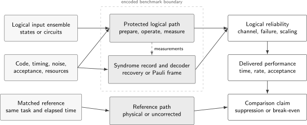
A logical benchmark compares a complete protected path with a declared reference. The state ensemble, timing, syndrome record, decoder, acceptance rule, and resources remain inside the boundary. Reliability without delivered rate or a matched denominator is only part of the result.
Choose the Logical Object
Section titled “Choose the Logical Object”Memory
Section titled “Memory”A logical-memory benchmark prepares an ensemble of encoded states, applies rounds of error correction or waits for time , decodes the record, and measures the logical output. It probes storage under a particular syndrome schedule and decoder. It does not establish the quality of logical gates or state factories.
For a one-logical-qubit Pauli memory, testing only probes logical bit flips but is insensitive to pure logical dephasing. A minimal cardinal-state ensemble includes eigenstates of , , and . Different axes can have different failure probabilities:
Noise bias may make that asymmetry intentional and useful, but averaging it away should be a declared choice. For multiple logical qubits, the benchmark must also detect correlated logical failures rather than report only marginal per-qubit rates.
Preparation and measurement
Section titled “Preparation and measurement”Logical state preparation and logical measurement are operations in their own right. A preparation benchmark should say whether verification, repeated checks, or postselection is included. A measurement benchmark should report the logical confusion matrix
including erasure or rejection outcomes when present. Averaging and can hide strong asymmetry.
If preparation and measurement surround every tested gate, their errors can be absorbed into fitted nuisance parameters only under a stable model. Direct logical process tomography exposes more structure but scales exponentially with the number of logical qubits and remains sensitive to its own SPAM model.
Logical gates and gadgets
Section titled “Logical gates and gadgets”A logical gate benchmark must define the gadget boundary. Does it include leading and trailing error correction, ancilla preparation, repeated parity measurements, decoding, feed-forward, injection, state transport, and factory retries? The gate’s operational channel changes when the boundary changes.
For fault-tolerance claims, benchmark both nominal noise and controlled fault injections. High average fidelity does not show error containment. A fault-tolerant gadget should respond to every fault set within its design order without allowing an uncorrectable output error, subject to the stated code and input conditions. Fault-Tolerant Gates owns that structural contract.
Integrated logical circuits
Section titled “Integrated logical circuits”An encoded circuit benchmark composes preparations, gates, measurements, factories, decoders, and controller decisions. It is more representative than an idle memory but harder to diagnose. The logical circuit family should span width, protected depth, non-Clifford demand, entanglement structure, and reaction depth rather than select one favorable demonstration.
Algorithmic Benchmarking owns the further step from a logical circuit to a task-level answer, including input access, output accuracy, classical comparison, and cost per accepted solution.
Name the Denominator
Section titled “Name the Denominator”A logical failure probability is a ratio
but the logical opportunity in the denominator may be:
- one syndrome-extraction round;
- one complete QEC cycle;
- one logical qubit-round;
- one prepared or measured logical state;
- one protected gate or lattice-surgery operation;
- one Clifford in a randomized sequence;
- one spacetime volume; or
- one complete logical circuit.
These quantities are not interchangeable. For small independent failure probabilities , a circuit with opportunities of class has
The approximation fails when faults are correlated, when recovery couples opportunities, or when the operation classes overlap. A per-round number cannot be multiplied by gate count unless the gate genuinely consists of those rounds under the same noise and decoding conditions.
Per round and per unit time
Section titled “Per round and per unit time”Suppose a binary logical observable flips independently with probability per cycle. After cycles, its correlation decays as
With preparation and measurement nuisance parameters, a common fit is
and do not magically remove SPAM; they model fixed boundary effects. Multiple exponentials, oscillations, leakage, nonstationarity, and decoder memory can invalidate this form.
If one cycle lasts , the equivalent continuous-time parity-flip rate is
for . Comparing codes only per cycle can favor a slower cycle; comparing only per second can hide a useful architectural primitive. Report both.
Boundary rounds
Section titled “Boundary rounds”Initialization and final measurement rounds often have different fault mechanisms from steady-state memory rounds. If the probability of a correct logical outcome after bulk rounds is fit as
then describes a bulk decay mode only if the boundaries are stable and the chosen range has reached that mode. Quoting from two sequence lengths without residual checks can turn transients into a steady-state error rate.
Logical Channels and Metrics
Section titled “Logical Channels and Metrics”Pauli failure is task-specific
Section titled “Pauli failure is task-specific”In a stabilizer memory with a Pauli-frame decoder, a trial fails when the inferred recovery differs from the actual fault by a nontrivial logical operator. This produces a logical Pauli distribution
The scalar is meaningful for that Pauli-channel model. Under coherent logical rotations, leakage, or non-Markovian behavior, one number does not describe how errors compose.
Logical process representation
Section titled “Logical process representation”For logical qubits with logical Pauli basis , a Pauli transfer matrix can represent the decoded channel:
The diagonal entries describe contraction of Pauli observables; off-diagonal entries expose coherent mixing and non-Pauli structure. Logical process tomography can estimate this matrix for small , but its preparation, measurement, gauge, and sampling costs grow quickly.
Average logical fidelity is useful for a declared ensemble. It should not be substituted for a worst-case error bound without assumptions. Coherent errors can have average infidelity quadratic in a small rotation angle while their worst-case effect is linear in that angle. Threshold and resource models must use a metric compatible with their noise assumptions.
Leakage and loss
Section titled “Leakage and loss”The code space is not always preserved. Report at least
An erasure flag can help the decoder and is operationally different from unflagged leakage. A protocol that discards every detected loss measures a conditional logical channel plus an acceptance rate, not an unconditional error-corrected channel.
Detection, Correction, and Postselection
Section titled “Detection, Correction, and Postselection”Detection events are evidence that the syndrome circuit is sensitive to faults. They are not themselves logical failures, and a low detection-event rate is not necessarily good: a broken check can report no events while failing to protect the state.
Three benchmark modes should be named separately:
- Detection: acquire flags or syndrome changes and characterize their statistics without attempting to deliver every logical output.
- Postselected detection: accept only a declared subset of records and report the conditional output quality and acceptance.
- Correction: decode every in-scope record, update a frame or recovery, and score the delivered logical output.
If is the acceptance probability and the logical failure probability conditioned on acceptance, one trial has probabilities
The pair must be reported. If rejected trials are restarted, the mean number of attempts per accepted result is under independent, stationary trials. A lower conditional error obtained by driving toward zero is not free error correction.
Selection can also bias the noise distribution. Accepted runs may exclude precisely the leakage, loss, or high-weight events that a scalable machine must handle. That may be appropriate for a heralded primitive, but the benchmark claim must stay conditional.
Scaling and Below-Threshold Evidence
Section titled “Scaling and Below-Threshold Evidence”Matched code-size comparisons
Section titled “Matched code-size comparisons”For code sizes and , define the measured suppression factor
means the larger tested code performs better for the declared metric. The comparison supports below-threshold behavior only when the code family, logical task, physical operating point, cycle definition, noise exposure, decoder information, and acceptance rule are matched. If the larger code gets a better-calibrated subset of hardware or a slower cycle, the change must be modeled rather than attributed solely to distance.
One favorable pair is finite-size evidence, not an asymptotic proof. Stronger evidence includes several increasing sizes, both logical bases, multiple round counts, stable suppression across time blocks, and a circuit-level model that predicts held-out data. Threshold Theorem explains why a finite crossing, a pseudothreshold, and an asymptotic threshold are distinct concepts.
Uncertainty in a suppression factor
Section titled “Uncertainty in a suppression factor”Because is a ratio, uncertainty in the smaller logical error can dominate. For approximately independent estimates with small relative error,
Near zero failures this approximation is poor; use a joint likelihood, Bayesian posterior with a declared prior, or profile/bootstrap interval that respects the binomial boundary. Report the confidence interval for , not only point estimates for each error rate.
Scaling in time as well as distance
Section titled “Scaling in time as well as distance”Logical memory should be tested over enough rounds to expose the steady-state regime and rare correlated events. Scaling only at one short duration can be dominated by preparation and readout. Scaling only at a very long duration can saturate near random guessing and lose sensitivity. A two-dimensional grid in distance and round count is more informative than one diagonal slice.
Break-Even Requires a Named Reference
Section titled “Break-Even Requires a Named Reference”A logical system reaches break-even when it outperforms a declared unencoded or physical reference on a matched task and metric. For an error probability,
is a gain relative to baseline ; indicates break-even. The result is incomplete unless the denominator is named.
Possible references include:
- the best physical carrier among the encoded components;
- the mean or median constituent carrier;
- an unencoded carrier exposed for the same wall-clock time;
- an uncorrected encoded state using the same preparation and measurement;
- the best available physical implementation of the same gate; or
- a module-level reference that includes ancillas, controls, and retries.
No one reference answers every engineering question. A fair comparison aligns the input ensemble, elapsed time, measurement rule, acceptance policy, and access to calibration information. Comparing one logical QEC round with one physical gate is not a memory break-even test.
Break-even and error suppression are logically independent. Increasing distance can reduce while the logical memory still underperforms the best physical carrier. A fixed code can beat a physical reference without belonging to a scalable family. Neither statement alone establishes a fault-tolerant universal gate set.
Benchmarking Logical Gates
Section titled “Benchmarking Logical Gates”Direct logical tomography
Section titled “Direct logical tomography”For one or a few logical qubits, prepare a spanning set of logical inputs, apply the complete gate gadget, and measure a spanning set of logical observables. This reconstructs or bounds the logical process. Include idle or identity gadgets of equal duration, because a high gate fidelity can coexist with a poor logical memory and vice versa.
Tomography is diagnostic but not scalable. It also depends on trusted logical preparations and measurements unless gate-set methods are used, and its result may be gauge-dependent. The full syndrome record can help diagnose faults but must not be used to tune the gate on the held-out test data.
Logical randomized benchmarking
Section titled “Logical randomized benchmarking”Logical randomized benchmarking samples sequences from a logical gate group, implements each logical element fault tolerantly, appends an inversion, and fits survival versus sequence length. Under the usual single-mode model,
For a -dimensional logical system, the associated average error parameter is
The implementation must specify how a sampled logical Clifford is compiled, where error correction occurs, whether syndrome ancillas are reset, and which records are accepted. The sequence ensemble measures an average over that implemented distribution, not every logical gate and not an arbitrary algorithm.
Logical QEC machinery can preserve hidden syndrome memory between gates, so even gate- and time-independent physical noise can produce nonexponential logical-RB behavior. Residuals, alternative decay models, leakage observables, and sequence-to-sequence variation are therefore essential checks.
Interleaved and cycle-level tests
Section titled “Interleaved and cycle-level tests”An interleaved logical benchmark alternates a target logical gadget with reference randomizers. Its interpretation inherits the assumptions and bounds of physical interleaved RB. A logical cycle benchmark instead targets a parallel protected layer and can expose simultaneous-operation and crosstalk effects. In both cases, compare against an equal-duration logical identity and report the compiled primitive distribution.
Non-Clifford gates require special care. State injection can move error from a resource state into the data; adaptive corrections add reaction latency; factory postselection changes acceptance. Benchmark the delivered injected gate or magic state and separately report factory quality, throughput, and resource cost.
Decoder as Part of the Benchmark
Section titled “Decoder as Part of the Benchmark”The decoder converts the syndrome record into a logical decision, so changing it changes the measured logical channel. Report:
- decoder algorithm and version;
- the exact observations supplied, including soft readout, erasure, leakage, and future-round information;
- training, calibration, and hyperparameter data;
- whether decoding is offline, streaming, or deadline constrained;
- handling of ties, timeouts, and decoder failures; and
- latency and throughput distributions when they affect execution.
Training and evaluation records must be separated. A decoder fitted to every observed logical outcome can memorize drift or exploit information unavailable in operation. Time-ordered holdout blocks are often more revealing than a random shot split when calibration drifts.
An offline decoder with access to syndrome rounds after the nominal endpoint can estimate a retrospective memory channel. A real-time decoder that must choose a feed-forward action before a deadline measures an operational gate or computation channel. Both are legitimate, but they answer different questions.
Benchmark the decoder jointly with the physical implementation for delivered logical performance, and benchmark it separately on frozen datasets for algorithmic comparison. This prevents a faster but less accurate decoder from being ranked by accuracy alone, or a more accurate offline decoder from being presented as deployable without a latency analysis.
Statistical Design
Section titled “Statistical Design”Failures are binomial only under a contract
Section titled “Failures are binomial only under a contract”If independent, identically distributed logical opportunities produce failures, the binomial likelihood is
The estimator is simple, but QEC data often violate the independence assumption. Many rounds share one shot, qubits share a burst event, and chronological blocks share calibration drift. Treat the shot, sequence, device region, or time block as a sampling cluster when appropriate. Resampling individual rounds can produce confidence intervals that are much too narrow.
For ordinary binomial data, use Wilson, likelihood-ratio, or exact intervals rather than a symmetric normal interval near zero. Publish failure counts and opportunities so readers can recompute the interval.
Zero observed failures is not zero error
Section titled “Zero observed failures is not zero error”With failures in independent opportunities, the one-sided upper confidence bound at confidence is
At 95% confidence this is approximately . To bound a logical failure probability below with zero observed failures requires about three million independent opportunities, and correlation increases the effective requirement. Reporting “zero error” after a few thousand trials is therefore not evidence for a very low rate.
Sequences, shots, and time blocks
Section titled “Sequences, shots, and time blocks”For randomized logical circuits, three sample counts matter:
- independent logical sequences or circuit instances;
- repeated shots per fixed sequence; and
- chronological repetitions across recalibration or drift blocks.
More shots reduce projection noise for the chosen sequences. They do not measure sequence-to-sequence variability or long-time drift. A hierarchical model or nested bootstrap should reflect all sampled levels.
Rare-event simulation
Section titled “Rare-event simulation”When direct experiment or Monte Carlo cannot reach the target logical error rate, importance sampling, splitting, fault injection, or extrapolation may be used. Report the proposal distribution, likelihood weights, effective sample size, fault-order truncation, and validation region. A simulated logical failure estimate is evidence about the declared model, not direct evidence that hardware has the same tail.
Stopping and multiplicity
Section titled “Stopping and multiplicity”Predeclare sequence lengths, code sizes, primary metrics, stopping rules, and comparisons. Searching many decoder settings, bases, time windows, and postselection thresholds and reporting only the best one creates selection bias. Use a validation set or adjust uncertainty for the selection process.
Reliability Must Travel with Rate and Resources
Section titled “Reliability Must Travel with Rate and Resources”A logical primitive is useful only if it can deliver outputs. Report the physical and classical footprint, elapsed time, acceptance, and throughput beside reliability. If one trial takes , acceptance is , and accepted logical failure is , the rate of accepted correct outputs under stationary serial trials is
Parallel hardware changes the numerator and footprint together. A benchmark should therefore report a performance vector such as
not collapse everything into one score. Resource Estimation explains how these measured primitive quantities enter an application-scale cost model.
Classical decoding is part of the resource boundary when it is necessary to interpret or control the logical state. Report acquisition bandwidth, compute hardware, latency tails, backlog, and energy when they constrain the experiment. “Real time” should mean that the full closed loop meets the declared deadline, not merely that one decoder kernel is fast in isolation.
Worked Benchmark: Suppression Without Break-Even
Section titled “Worked Benchmark: Suppression Without Break-Even”Suppose matched logical-memory experiments produce the following independent window counts:
| Distance | Opportunities | Failures | Cycle time |
|---|---|---|---|
| 3 | 3600 | ||
| 5 | 1200 | ||
| 7 | 960 |
The per-cycle estimates are
The suppression factors are
Approximate binomial standard errors are , , and , respectively. A real analysis would use clustered intervals if windows share shots or drift blocks, then propagate the joint uncertainty to each ratio.
Per-time rates are approximately
Thus both per-cycle and per-time metrics improve with distance. Now compare distance 7 with a physical reference that fails with probability over the same interval and matched state ensemble. The break-even gain is
The logical family shows finite-size error suppression, yet the distance-7 memory has not beaten this physical reference. That is a coherent result, not a contradiction. It also says nothing about protected-gate quality until those gates are benchmarked.
A Minimum Logical Benchmark Suite
Section titled “A Minimum Logical Benchmark Suite”No single protocol is complete. A defensible suite for an encoded processor contains at least:
- Syndrome integrity: detection-event rates, correlations, leakage or loss flags, reset behavior, and response to injected faults.
- Logical memory: all relevant logical axes over multiple round counts, code sizes, time blocks, and simultaneous-load conditions.
- Scaling: matched suppression factors with uncertainty and finite-size caveats.
- Break-even: one or more named references aligned in task, time, acceptance, and measurement.
- Logical SPAM: preparation and measurement confusion or channel metrics, including rejected outcomes.
- Logical gates: identity and target gadgets, random-sequence or cycle-level tests, and controlled fault injection.
- Integrated circuits: representative entangling, adaptive, and non-Clifford workloads with end-to-end logical scoring.
- Delivery metrics: cycle and reaction time, decoder latency and throughput, physical footprint, acceptance, and correct-output rate.
The suite should include negative controls. Disable correction, use a simpler decoder, omit soft information, or replace a fault-tolerant gadget with a non-fault-tolerant one while keeping the task matched. These ablations identify which part of the stack produced the improvement.
Common Mistakes
Section titled “Common Mistakes”Calling detection correction
Section titled “Calling detection correction”A syndrome response shows sensitivity to faults. Improvement of the decoded logical channel shows correction. Postselected improvement is conditional and must include acceptance.
Reporting a denominator-free error rate
Section titled “Reporting a denominator-free error rate”Per round, per second, per logical Clifford, and per circuit answer different questions. State the opportunity count and operation boundary.
Testing one logical basis
Section titled “Testing one logical basis”Preserving can miss dephasing entirely. Use a state ensemble matched to the claimed logical channel.
Treating a fitted exponential as guaranteed
Section titled “Treating a fitted exponential as guaranteed”Syndrome memory, leakage, coherent errors, drift, and boundary transients can produce several modes or nonexponential behavior. Inspect residuals and vary the fit window.
Using the test set to tune the decoder
Section titled “Using the test set to tune the decoder”Decoder weights, neural parameters, postselection thresholds, and calibration choices must be fixed before held-out evaluation. Random splitting can still leak chronological drift.
Equating suppression with break-even
Section titled “Equating suppression with break-even”compares two encoded systems. Break-even compares an encoded system with a named reference. Neither alone proves a universal logical gate set.
Ignoring time and acceptance
Section titled “Ignoring time and acceptance”A lower error per cycle can come from a much slower cycle. A lower conditional error can come from rejecting most trials. Report delivery rate and resource cost.
Claiming zero logical error
Section titled “Claiming zero logical error”Zero observed failures implies an upper confidence bound controlled by sample size. It is never evidence for exactly zero error.
Comparing offline and real-time decoding
Section titled “Comparing offline and real-time decoding”Future syndrome access and unlimited latency can improve retrospective decoding. An adaptive computation must satisfy the online information and deadline contract.
Exercises
Section titled “Exercises”1. Convert a memory decay to error per cycle
Section titled “1. Convert a memory decay to error per cycle”A logical parity correlation decays by a fitted factor per cycle. Find the independent parity-flip probability per cycle.
Solution
The model uses , so
This conversion is valid only for the stated single-mode binary-flip model. It is not a general conversion from every fitted decay to a logical channel.
2. Compare per-cycle and per-time performance
Section titled “2. Compare per-cycle and per-time performance”Code A has per cycle. Code B has per cycle. Which is better per cycle and which is better per unit time in the small-error limit?
Solution
Code B has the smaller error per cycle. The approximate rates are
Code B is also better per unit time. The question remains meaningful because the cycle durations were reported.
3. Bound zero observed failures
Section titled “3. Bound zero observed failures”A benchmark observes no logical failures in independent trials. Find the approximate one-sided 95% upper bound on . Does this establish at 95% confidence?
Solution
Using gives
No. The data are compatible with probabilities above at that confidence. Correlation would reduce the effective sample size and weaken the bound further.
4. Account for postselection
Section titled “4. Account for postselection”A detected-code experiment accepts 20% of trials and has conditional logical failure . Each trial takes 5 ms. Find the rate of accepted correct outputs and the mean number of attempts per accepted output.
Solution
The correct-output rate is
The mean number of attempts per accepted output is . Reporting only would hide most of the delivery cost.
5. Distinguish scaling and break-even
Section titled “5. Distinguish scaling and break-even”A distance-3 memory has and distance 5 has under matched conditions. The physical reference has . State the supported claims.
Solution
The measured suppression factor is
Thus the larger code suppresses the declared logical error under the matched finite-size test. Its break-even gain is
so it does not beat that physical reference. Neither comparison establishes logical-gate fault tolerance.
6. Diagnose a nonexponential logical-RB curve
Section titled “6. Diagnose a nonexponential logical-RB curve”A logical randomized benchmark has oscillatory residuals around a one- exponential fit, and the oscillation phase correlates with the syndrome state left by the previous logical Clifford. What assumption is suspect, and what should be reported?
Solution
The single stationary decay-mode assumption is suspect. Syndrome ancillas, decoder state, or frame history can retain memory and act as hidden degrees of freedom coupled to the logical system. Report the residuals, sequence-level data, syndrome-reset policy, and alternative decay model; do not reduce the curve to one logical error parameter without a validated model.
7. Design a fair logical-gate comparison
Section titled “7. Design a fair logical-gate comparison”List the controls needed to compare a fault-tolerant logical Hadamard gadget with a non-fault-tolerant implementation.
Solution
Use the same logical code and input ensemble; define both gadget boundaries; match or explicitly report elapsed time, syndrome rounds, preparation and measurement, decoder information, acceptance, and physical operating point; include equal-duration identity controls; use held-out trials; report logical channel metrics and uncertainty; inject representative single faults to test containment; and account for all qubit, controller, and retry resources. A fidelity improvement under nominal noise and a containment improvement under fault injection are complementary results.
8. Plan a distance-scaling experiment
Section titled “8. Plan a distance-scaling experiment”Design a minimal experiment that can distinguish boundary SPAM from bulk logical memory decay while testing suppression from distance 3 to distance 5.
Solution
Use matched physical operating conditions and syndrome schedules for both distances; prepare at least the logical and eigenstate ensembles; sample several round counts including zero or a short boundary control and enough long counts to expose bulk decay; interleave distances chronologically to control drift; freeze the decoder before evaluation; record all syndrome, leakage, acceptance, and timing data; fit boundary amplitudes separately from bulk decay; inspect residuals; estimate clustered confidence intervals; and report the suppression-factor interval in both per-cycle and per-time units.
Research Status
Section titled “Research Status”The need to measure complete logical channels and declare denominators is settled methodology. The best scalable protocols are still developing. Logical randomized benchmarking can inherit hidden syndrome memory; non-Clifford resource states can be expensive to test at the multiplicative precision required by fault-tolerant budgets; and extremely low logical error rates make direct sampling costly. Scalable accreditation, rare-event simulation, and benchmark suites for integrated logical processors remain active research.
Experimental capabilities are also changing quickly. Increasing-distance surface-code memories, bosonic break-even results, protected logical gates, real-time decoding, loss-aware operation, and multi-logical-qubit processors probe different parts of the benchmark suite. Their current evidence belongs in Error-Correction Case Studies and the Fault-Tolerant Quantum Computing Frontier.
Further Connections
Section titled “Further Connections”- Why Quantum Error Correction Is Possible defines the ideal correctability condition behind the measured logical channel.
- Decoders develops logical-class inference, decoder families, soft information, model mismatch, and real-time systems metrics.
- Threshold Theorem distinguishes a finite suppression measurement from an asymptotic accuracy threshold.
- Fault-Tolerant Gates supplies the error-containment property that nominal logical fidelity alone cannot establish.
- Surface Code develops repeated checks, spacetime detection events, logical strings, distance, and code-specific suppression.
- Resource Estimation consumes measured logical failure, timing, throughput, and footprint as inputs to application-scale projections.
- Randomized Benchmarking derives reference and interleaved RB, nuisance parameters, sampling hierarchy, and failure modes.
- Cycle Benchmarking develops dressed-cycle estimands and simultaneous-layer protocols that can be lifted to logical cycles.
- Why Benchmarking Is Hard explains benchmark boundaries, context dependence, drift, compiler freedom, and selection risk across the whole stack.
- Reporting Standards supplies the provenance, uncertainty, correction, and artifact record for published logical results.
- Error-Correction Case Studies applies the contract to dated repetition-code, surface-code, and bosonic experiments.
References
Section titled “References”- J. Combes, C. Granade, C. Ferrie, and S. T. Flammia, “Logical randomized benchmarking,” arXiv:1702.03688 (2017), arXiv:1702.03688.
- A. Ceasura, P. Iyer, J. J. Wallman, and H. Pashayan, “Non-exponential behaviour in logical randomized benchmarking,” arXiv:2212.05488 (2022), arXiv:2212.05488.
- E. Knill et al., “Randomized benchmarking of quantum gates,” Physical Review A 77, 012307 (2008), doi:10.1103/PhysRevA.77.012307.
- E. Magesan, J. M. Gambetta, and J. Emerson, “Scalable and robust randomized benchmarking of quantum processes,” Physical Review Letters 106, 180504 (2011), doi:10.1103/PhysRevLett.106.180504.
- J. Helsen, I. Roth, E. Onorati, A. H. Werner, and J. Eisert, “General framework for randomized benchmarking,” PRX Quantum 3, 020357 (2022), doi:10.1103/PRXQuantum.3.020357.
- R. Harper and S. T. Flammia, “Fault-tolerant logical gates in the IBM quantum experience,” Physical Review Letters 122, 080504 (2019), doi:10.1103/PhysRevLett.122.080504.
- Google Quantum AI, “Suppressing quantum errors by scaling a surface code logical qubit,” Nature 614, 676–681 (2023), doi:10.1038/s41586-022-05434-1.
- Google Quantum AI and Collaborators, “Quantum error correction below the surface code threshold,” Nature 638, 920–926 (2025), doi:10.1038/s41586-024-08449-y.
- J. Kelly et al., “State preservation by repetitive error detection in a superconducting quantum circuit,” Nature 519, 66–69 (2015), doi:10.1038/nature14270.
- L. Egan et al., “Fault-tolerant control of an error-corrected qubit,” Nature 598, 281–286 (2021), doi:10.1038/s41586-021-03928-y.
- C. Ryan-Anderson et al., “Realization of real-time fault-tolerant quantum error correction,” Physical Review X 11, 041058 (2021), doi:10.1103/PhysRevX.11.041058.
- J. F. Marques et al., “Logical-qubit operations in an error-detecting surface code,” Nature Physics 18, 80–86 (2022), doi:10.1038/s41567-021-01423-9.
- P. Reinhold et al., “Error-corrected gates on an encoded qubit,” Nature Physics 16, 822–826 (2020), doi:10.1038/s41567-020-0931-8.
- M. H. Abobeih et al., “Fault-tolerant operation of a logical qubit in a diamond quantum processor,” Nature 606, 884–889 (2022), doi:10.1038/s41586-022-04819-6.
- E. H. Chen et al., “Calibrated decoders for experimental quantum error correction,” Physical Review Letters 128, 110504 (2022), doi:10.1103/PhysRevLett.128.110504.
- V. V. Sivak et al., “Real-time quantum error correction beyond break-even,” Nature 616, 50–55 (2023), doi:10.1038/s41586-023-05782-6.
- Z. Ni et al., “Beating the break-even point with a discrete-variable-encoded logical qubit,” Nature 616, 56–60 (2023), doi:10.1038/s41586-023-05784-4.
- S. Lee, M. Yuan, S. Chen, K. Tsubouchi, and L. Jiang, “Efficient benchmarking of logical magic state,” Physical Review Letters 136, 050602 (2026), doi:10.1103/fwjt-mw2c.