GKP Codes

A Gottesman–Kitaev–Preskill code, or GKP code, embeds a finite logical system in one or more oscillator modes by imposing a lattice of phase-space translation symmetries. Small continuous shifts of the quadratures become modular syndromes. Recovery rounds those analog shifts to a lattice cell, thereby converting a continuum of physical errors into discrete logical Pauli errors that an outer code can process.

That compact description hides three distinct layers:

1. the ideal code is an exact translation-stabilizer code whose codewords are nonnormalizable Dirac combs;
2. a finite-energy code replaces the comb by finite-width peaks under a decaying envelope and is only approximately invariant under ideal translations;
3. an implemented protocol adds noisy state preparation, ancillas, syndrome extraction, decoding, feedback or autonomous pumping, and gates.

Statements about one layer do not automatically hold at the next.

Bosonic Codes is the canonical home for the common oscillator-code and recovery framework. Bosonic Qubits owns the oscillator–ancilla module, platform comparisons, and hardware evidence. Continuous-Variable Quantum Computation owns abstract mode computation and continuous-variable cluster-model semantics. Continuous-Variable Platforms owns optical and microwave cluster architectures, physical resource generation, and hardware evidence. This page owns GKP lattice conventions, ideal and finite- energy codewords, displacement distance, modular syndromes, analog decoding, code-specific gate options, variants, and fault-tolerance boundaries.

Bosonic and Encoded Computation Models owns the code-family-independent audit that composes a declared physical oscillator program before extracting its induced logical channel, leakage, rejection, recovery, frame, and resource ledger. This page retains the GKP lattice, states, syndromes, analog decoding, recovery, family-specific logical gates, and thresholds.

Quantum Error Correction and Fault Tolerance treats a GKP code as one phase-space encoding inside a complete protection record; this page retains lattice conventions, modular syndromes, finite-energy effects, analog decoding, recovery, logical gates, variants, evidence, and resources.

Phase-Space Convention

One oscillator has annihilation operator $a$ and dimensionless quadratures

$$\begin{gathered} q = \frac{a+a^\dagger}{\sqrt2}, \qquad p = \frac{a-a^\dagger}{i\sqrt2}, \\ [q,p]=i, \qquad n=a^\dagger a = \frac{q^2+p^2-1}{2}. \end{gathered}$$

All distances below use these $q,p$ coordinates. A Weyl displacement is

$$W(u,v) = \exp\!\left[ i(vq-up) \right].$$

It shifts the quadrature means by

$$W(u,v)^\dagger qW(u,v)=q+u, \qquad W(u,v)^\dagger pW(u,v)=p+v.$$

The multiplication law is

$$\begin{aligned} W(u,v)W(u',v') &= \exp\!\left[ -\frac{i}{2} (uv'-vu') \right] \\ &\quad\times W(u+u',v+v'). \end{aligned}$$

Consequently,

$$\begin{aligned} W(u,v)W(u',v') &= e^{-i(uv'-vu')} \\ &\quad\times W(u',v')W(u,v). \end{aligned}$$

Two displacements commute when the signed phase-space area $uv'-vu'$ is an integer multiple of $2\pi$. This area rule is the geometric origin of the stabilizer lattice.

Convention warning

Some papers use $[q,p]=i/2$, or plot the complex displacement amplitude $\alpha=(u+iv)/\sqrt2$ instead of $(u,v)$. In those conventions every quoted lattice length changes by a factor of $\sqrt2$. A squeezing or distance number is not portable until the quadrature normalization is stated.

Ideal Square GKP Qubit

The square GKP qubit is the simultaneous $+1$ generalized eigenspace of

$$S_Z = W(0,2\sqrt\pi) = e^{i2\sqrt\pi q},$$

and

$$S_X = W(2\sqrt\pi,0) = e^{-i2\sqrt\pi p}.$$

The generators commute because their enclosed area is $4\pi$. The subscripts refer to the associated logical Pauli convention: $S_Z$ is a full momentum translation and $S_X$ is a full position translation.

In the position representation, a convenient logical basis is

$$\langle q|0_L\rangle \propto \sum_{s\in\mathbb Z} \delta\!\left( q-2s\sqrt\pi \right),$$

and

$$\langle q|1_L\rangle \propto \sum_{s\in\mathbb Z} \delta\!\left( q-(2s+1)\sqrt\pi \right).$$

Logical zero occupies even multiples of $\sqrt\pi$; logical one occupies odd multiples. Their sum and difference have the reciprocal combs

$$\langle p|+_L\rangle \propto \sum_{s\in\mathbb Z} \delta\!\left( p-2s\sqrt\pi \right),$$

and

$$\langle p|-_L\rangle \propto \sum_{s\in\mathbb Z} \delta\!\left( p-(2s+1)\sqrt\pi \right).$$

The logical Pauli translations are half the stabilizer length:

$$Z_L = W(0,\sqrt\pi) = e^{i\sqrt\pi q},$$

and

$$X_L = W(\sqrt\pi,0) = e^{-i\sqrt\pi p}.$$

They satisfy

$$Z_LX_L=-X_LZ_L,$$

commute with both stabilizers, and act as

$$\begin{aligned} Z_L|0_L\rangle&=|0_L\rangle, & Z_L|1_L\rangle&=-|1_L\rangle, \\ X_L|0_L\rangle&=|1_L\rangle, & X_L|1_L\rangle&=|0_L\rangle. \end{aligned}$$

The ideal construction can be summarized as follows.

item	square GKP qubit
physical carrier	one oscillator mode
logical subspace	simultaneous ideal $+1$ eigenspace of two commuting translations
stabilizers	$S_Z=e^{i2\sqrt\pi q}$ and $S_X=e^{-i2\sqrt\pi p}$
logical Paulis	$Z_L=e^{i\sqrt\pi q}$ and $X_L=e^{-i\sqrt\pi p}$
displacement distance	$d_{\rm disp}=\sqrt\pi$ in the stated $(q,p)$ coordinates
ideal correctable cell	$\lvert u\rvert<\sqrt\pi/2$ and $\lvert v\rvert<\sqrt\pi/2$
syndrome	stabilizer phases, equivalently $u$ and $v$ modulo $\sqrt\pi$
basic decoder	nearest point of the logical displacement lattice
ideal Clifford gates	Gaussian symplectic transformations
non-Clifford route	magic-state injection, a nonlinear phase resource, or code-aware optimal control

There is a crucial mathematical qualification: the Dirac combs are distributions, not vectors of the oscillator Hilbert space. They have no finite normalization and no finite mean energy. The ideal code is an exact algebraic reference, not a laboratory state.

Lattice Geometry and Displacement Distance

The square stabilizer lattice is

$$\Lambda_{\rm S} = 2\sqrt\pi\,\mathbb Z^2.$$

The displacements that commute with every stabilizer form its symplectic dual,

$$\Lambda_{\rm S}^{\perp} = \sqrt\pi\,\mathbb Z^2.$$

The quotient

$$\Lambda_{\rm S}^{\perp}/\Lambda_{\rm S} \cong \mathbb Z_2\times\mathbb Z_2$$

contains the four logical displacement cosets $I$, $X$, $Z$, and $Y$. The shortest displacement in the dual lattice that is not a stabilizer has length

$$d_{\rm disp} = \min_{\lambda\in \Lambda_{\rm S}^{\perp}\setminus\Lambda_{\rm S}} \|\lambda\| = \sqrt\pi.$$

This is a phase-space distance, not a Hamming weight. Its operational meaning depends on a metric and a decoder. For isotropic additive Gaussian noise, Euclidean nearest-lattice decoding is natural and the Voronoi cell around the identity is

$$\mathcal V_I = \left[ -\frac{\sqrt\pi}{2}, \frac{\sqrt\pi}{2} \right) \times \left[ -\frac{\sqrt\pi}{2}, \frac{\sqrt\pi}{2} \right).$$

For anisotropic or correlated noise, the likelihood contours are not circles, and Euclidean distance need not be the correct decoding metric.

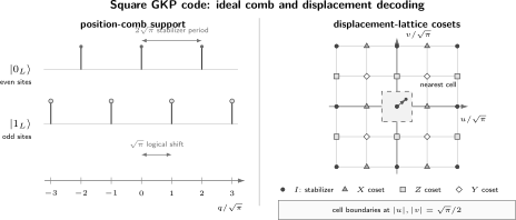
Left: the ideal logical basis alternates on a position comb with logical spacing $\sqrt\pi$ and stabilizer period $2\sqrt\pi$. Right: the commuting displacement lattice splits into $I$, $X$, $Z$, and $Y$ cosets. The shaded square is the nearest-lattice correction cell around $I$; crossing one of its boundaries can leave a logical Pauli after recovery. This is displacement space, not a Wigner-function plot of a physical finite-energy state.

Correctable Shifts and Modular Syndromes

Suppose a displacement error $W(u,v)$ acts on an ideal code state. Weyl commutation gives

$$\begin{aligned} S_ZW(u,v)|\psi_L\rangle &= e^{i2\sqrt\pi u} W(u,v)|\psi_L\rangle, \\ S_XW(u,v)|\psi_L\rangle &= e^{-i2\sqrt\pi v} W(u,v)|\psi_L\rangle. \end{aligned}$$

The two stabilizer phases reveal

$$u\bmod\sqrt\pi, \qquad v\bmod\sqrt\pi,$$

without revealing the encoded amplitudes. Choose centered representatives

$$\tilde u,\tilde v \in \left[ -\frac{\sqrt\pi}{2}, \frac{\sqrt\pi}{2} \right).$$

Applying $W(-\tilde u,-\tilde v)$ leaves

$$W(m\sqrt\pi,n\sqrt\pi), \qquad m,n\in\mathbb Z,$$

up to a global phase. The parities of $m$ and $n$ determine the residual logical Pauli:

parity of $(m,n)$	residual logical operator
even, even	$I_L$
odd, even	$X_L$
even, odd	$Z_L$
odd, odd	$Y_L$ up to phase

If the physical shift lies strictly inside $\mathcal V_I$, then $m=n=0$ and ideal recovery is exact. At a cell boundary, two corrections are equally near; no decoder can resolve the ambiguity without a prior or additional information.

Two decoding examples

For

$$u=0.37\sqrt\pi, \qquad v=-0.18\sqrt\pi,$$

the centered residue is the shift itself. Recovery returns the state to the identity coset.

For

$$u=0.63\sqrt\pi, \qquad v=-0.18\sqrt\pi,$$

the measured position-shift residue is

$$\tilde u=-0.37\sqrt\pi.$$

The corresponding correction leaves a net position translation $\sqrt\pi$, hence a logical $X_L$. The syndrome was measured perfectly; the logical error arose because the physical shift crossed a decoding boundary.

Gaussian displacement noise

Let a position shift be Gaussian,

$$f_\sigma(u) = \frac{1}{\sqrt{2\pi\sigma^2}} \exp\!\left( -\frac{u^2}{2\sigma^2} \right).$$

Nearest-lattice decoding produces a logical $X$ whenever $u$ lies in a cell centered on an odd multiple of $\sqrt\pi$:

$$\begin{aligned} p_X^{(q)} &= \sum_{\substack{m\in\mathbb Z\\m\ {\rm odd}}} \int_{(m-1/2)\sqrt\pi}^{(m+1/2)\sqrt\pi} f_\sigma(u)\,du. \end{aligned}$$

At small $\sigma$, the nearest two wrong cells dominate, giving

$$p_X^{(q)} \simeq \operatorname{erfc}\!\left( \frac{\sqrt\pi}{2\sqrt2\,\sigma} \right),$$

with exponentially smaller corrections from farther even and odd cells. The same calculation applies to momentum shifts and logical $Z$ errors.

This formula is a channel model, not a universal performance law. Finite energy, noisy ancillas, loss, rotations, and repeated measurements alter the distribution and can correlate the two axes.

Analog information

A modular outcome is more informative than a hard Pauli decision. The general decoder contract explains how soft records enter logical-class inference. For the square GKP code, given a centered residue $r$ and a Gaussian prior, the likelihoods that the hidden lattice index is even or odd are

$$\begin{aligned} P_{\rm even}(r) &\propto \sum_{\substack{k\in\mathbb Z\\k\ {\rm even}}} \exp\!\left[ -\frac{(r+k\sqrt\pi)^2}{2\sigma^2} \right], \\ P_{\rm odd}(r) &\propto \sum_{\substack{k\in\mathbb Z\\k\ {\rm odd}}} \exp\!\left[ -\frac{(r+k\sqrt\pi)^2}{2\sigma^2} \right]. \end{aligned}$$

The log-likelihood ratio

$$\Lambda(r) = \log \frac{P_{\rm even}(r)} {P_{\rm odd}(r)}$$

is large in magnitude near a cell center and approaches zero near a decision boundary. Passing this soft information to a concatenated surface-code or cluster-state decoder can outperform throwing it away and retaining only a binary syndrome.

Finite-Energy GKP States

No normalizable physical state is exactly invariant under both independent stabilizer translations. A common one-parameter finite-energy model applies a Gaussian envelope operator to an ideal codeword:

$$E_\Delta = e^{-\Delta^2 n}, \qquad |\mu_{\Delta}\rangle = \frac{ E_\Delta|\mu_L\rangle }{ \sqrt{ \langle\mu_L|E_\Delta^2|\mu_L\rangle } }.$$

For $\Delta>0$, the state is normalizable and has finite mean occupation. The ideal limit is $\Delta\to0$, in which the energy diverges.

Another useful model displays the two physical scales directly:

$$\begin{aligned} \langle q|\mu_{\sigma,\kappa}\rangle \propto \sum_{s\in\mathbb Z} & \exp\!\left[ -\frac{ (q-q_{s\mu})^2 }{4\sigma^2} \right] \\ &\times \exp\!\left[ -\frac{\kappa^2q_{s\mu}^2}{2} \right], \end{aligned}$$

where

$$q_{s\mu} = (2s+\mu)\sqrt\pi.$$

Here $\sigma^2$ is the probability variance of an isolated position peak in the negligible-overlap limit, while $\kappa^{-1}$ controls the broad envelope. Fourier transformation exchanges peak and envelope roles between the two quadratures. A one-parameter symmetric model ties these scales together; a general prepared state need not.

What finite energy changes

Finite energy is not a cosmetic preparation infidelity. It changes:

• exact stabilizer eigenvalues into distributions of modular outcomes;
• orthogonality and logical-state normalization;
• intrinsic decoding tails before additional environmental noise;
• mean occupation and sensitivity to photon loss;
• how Gaussian gates deform the envelope;
• the backaction tolerated from finite-strength syndrome extraction;
• which channel distance and recovery metric are physically meaningful.

The energy cost increases as peaks narrow. In a symmetric small-width regime, the mean occupation scales parametrically as

$$\bar n=O(\sigma^{-2}),$$

although the coefficient depends on the envelope convention.

Squeezing must name a convention

If $\sigma^2$ denotes the probability variance of an isolated quadrature peak and the vacuum variance is $1/2$, one common effective squeezing convention is

$$s_{\rm GKP} = -10\log_{10}(2\sigma^2) \ {\rm dB}.$$

Other papers infer an effective width from stabilizer expectation values, fit a global finite-energy state, or report optical input squeezing. Those numbers need not coincide. A defensible report states the quadrature normalization, estimator, peak model, envelope model, and uncertainty.

The subsystem viewpoint

The oscillator Hilbert space can be organized as a logical subsystem and a continuous stabilizer-syndrome subsystem,

$$\mathcal H_{\rm osc} \cong \mathbb C^2 \otimes \mathcal H_{\rm synd},$$

for the square qubit convention. This decomposition is useful because a finite-energy physical state need not lie in an exact two-dimensional subspace: its logical content and its modular displacement content can still be separated operationally. It also supports channel simulation without a prohibitively large Fock cutoff.

Syndrome Extraction and Recovery

The ideal algebra specifies what to measure, not how to measure it. Four broad recovery routes are common.

GKP-ancilla extraction

A prepared grid-state ancilla interacts with the data through a SUM or controlled-phase Gaussian coupling. Homodyne measurement of the ancilla returns one modular quadrature; a second ancilla or round obtains the conjugate syndrome. This is the oscillator analogue of Steane-style syndrome extraction.

The ancilla is not harmless. Its finite squeezing adds shift noise, coupling faults can propagate between modes, detector inefficiency broadens the outcome, and a badly displaced ancilla can introduce a logical error into the data. Fault-tolerant analysis must include those channels rather than treating the ancilla as an exact comb.

Teleportation-based recovery

An encoded Bell resource, Gaussian entangling operation, and homodyne measurements can teleport the logical state into a fresh mode while supplying both modular syndromes. The feedforward displacement completes recovery. This route can combine error correction, state refresh, and gate teleportation, but its cost includes resource-state yield, optical or microwave loss, detection, and feedforward latency.

Two-level-ancilla phase estimation

In circuit QED and trapped motion, a nonlinear two-level ancilla can control oscillator displacements. Ramsey-like or phase-estimation sequences map a stabilizer phase to the ancilla, followed by readout, reset, and feedback. Echoed conditional displacements can reduce unwanted entanglement and make weak dispersive coupling useful.

Repeated rounds need a decoder over the complete record. Ancilla relaxation, dephasing, thermal population, readout assignment, leakage, and reset failure can all become oscillator displacements or envelope distortions.

Autonomous stabilization

Engineered dissipation or repeated unconditional ancilla-reset cycles can pump the oscillator toward a finite-energy GKP manifold without recording a classical syndrome each round. Autonomous operation removes some measurement latency, but it does not remove the ancilla, reset channel, pumps, or steady-state deformation from the resource and error budgets.

A decoder is more than rounding

Single-round nearest-lattice rounding is optimal only under a symmetric, memoryless displacement model with ideal syndrome readout. A practical decoder may need:

• unequal $q$ and $p$ noise variances;
• correlated shifts and phase rotations;
• finite-energy syndrome priors;
• a hidden Markov model for repeated rounds;
• ancilla-state and reset flags;
• analog likelihoods rather than hard decisions;
• oscillator loss and leakage hypotheses;
• joint decoding with an outer qubit code;
• a declared response to out-of-model records.

For a general multimode lattice, maximum-likelihood decoding becomes a closest-vector problem in the appropriate symplectic dual lattice. Exact closest-vector decoding is hard for an unstructured large lattice, although important structured GKP and surface–GKP families admit efficient decoders.

Noise Beyond Additive Displacements

The GKP code is naturally adapted to displacement errors. Real oscillators also experience attenuation, heating, dephasing, Kerr evolution, control leakage, and correlated ancilla faults.

Photon loss

A pure-loss channel of transmissivity $\eta$ transforms one quadrature as

$$q_{\rm out} = \sqrt\eta\,q +\sqrt{1-\eta}\,q_{\rm env},$$

with the environment in vacuum for ideal attenuation. The channel both shrinks the lattice and adds noise. A quantum-limited phase-insensitive amplifier of gain $1/\eta$ placed after the loss restores the mean scale but adds another vacuum contribution. In the present normalization, the combined additive variance per quadrature is

$$\sigma_{\rm add}^2 = \frac{1-\eta}{\eta}.$$

This mapping is useful for analysis, but the amplifier is a physical noisy operation and finite-energy envelope deformation remains. The GKP code does not algebraically “correct one photon loss” in the same sense as a declared Fock-state loss code.

Rotation and dephasing

Number dephasing generates random rotations,

$$U_\theta=e^{-i\theta n}.$$

A point at phase-space radius $r$ moves transversely by approximately $r\theta$ for small $\theta$. Far-out peaks of a high-energy grid can therefore cross a decoding boundary even when $\theta$ is small. This is one reason energy constraints are essential in channel metrics and fault-tolerance statements.

Hamiltonian distortion and ancilla faults

Self-Kerr evolution shears the grid. Calibration error in a conditional displacement leaves coherent residual shifts. Ancilla decay during a controlled operation can produce a displacement whose size depends on the unknown jump time. These faults are not captured by one Gaussian variance; the decoder and recovery must use the measured device channel.

The 2026 comparison literature reinforces the general lesson: GKP and number-phase codes exchange advantage as the balance of loss and dephasing changes. There is no oscillator code that is uniformly optimal for every channel.

Logical Gates and Fault-Tolerance Options

For the ideal square code, important logical Clifford operations are Gaussian symplectic transformations.

logical operation	oscillator action	phase-space map
$X_L$, $Z_L$	half-lattice displacements	translate by $\sqrt\pi$ along one axis
Hadamard	quarter-period rotation	$(q,p)\mapsto(p,-q)$ up to convention
phase gate	quadratic shear	$(q,p)\mapsto(q,p+q)$
SUM	$e^{-iq_1p_2}$	$q_2\mapsto q_2+q_1$, $p_1\mapsto p_1-p_2$
Pauli measurement	homodyne plus modular decoding	resolve a logical comb coset

Gaussian Clifford gates map the ideal lattice to itself. Universality still requires a non-Clifford resource, such as a logical magic state, a cubic-phase resource, photon counting, adaptive measurement, or a code-aware nonlinear control pulse.

Ideal transversality is not enough

Finite-energy envelopes are not invariant under every ideal lattice automorphism. A shear can stretch one envelope direction; a two-mode gate can correlate the shift noise; loss during a gate can propagate through a SUM interaction. A fault-tolerant gate claim must state:

1. the finite-energy input family;
2. which data and ancilla faults are included;
3. whether error correction occurs before, during, or after the gate;
4. how analog outcomes are propagated to the outer decoder;
5. whether the logical error improves as code resources increase;
6. the complete operation cost and acceptance probability.

Concatenation

An inner GKP layer digitizes oscillator noise and supplies soft information. An outer surface, color, repetition, or cluster-state code suppresses the remaining logical Pauli errors:

$$\text{oscillator noise} \longrightarrow \text{GKP analog syndrome} \longrightarrow \text{logical Pauli likelihood} \longrightarrow \text{outer-code decoder}.$$

Threshold values quoted for surface–GKP or photonic cluster architectures are conditional on a state model, squeezing convention, loss model, gate noise, decoder, and architecture. They are not universal constants of “the GKP code.”

In 2026, a threshold theorem extended continuous-variable fault tolerance beyond the usual Gaussian-random-displacement idealization to a specified class of general Markovian-type noise. The result uses finite-energy states, energy-aware channel bounds, GKP gadgets, and an outer concatenated code. It is an important theoretical advance, not evidence that arbitrary unbounded noise or a present device lies below threshold.

Common Variants

Rectangular and biased lattices

A rectangular lattice trades correction radius between $q$ and $p$ while preserving the symplectic cell area. It can be advantageous when one quadrature is substantially noisier or when concatenation is designed around a biased logical channel. The decoder metric must use that asymmetry.

Hexagonal lattices

At fixed cell area, a hexagonal lattice has a larger Euclidean packing radius than a square lattice for isotropic shifts. This can lower ideal displacement error under an isotropic Gaussian model. Gate convenience, syndrome circuits, finite-energy preparation, and hardware anisotropy can reverse the comparison.

Square GKP qudits

A one-mode square GKP qudit of logical dimension $d$ has stabilizer spacing

$$\ell_d=\sqrt{2\pi d}$$

in the present $q,p$ coordinates, and logical spacing

$$\lambda_d = \sqrt{\frac{2\pi}{d}}.$$

The stabilizers and generalized Paulis may be chosen as

$$\begin{gathered} S_Z=e^{i\ell_d q}, \qquad S_X=e^{-i\ell_d p}, \\ Z_d=e^{i\lambda_d q}, \qquad X_d=e^{-i\lambda_d p}. \end{gathered}$$

With

$$\omega_d=e^{2\pi i/d},$$

they obey

$$Z_dX_d=\omega_d X_dZ_d.$$

The ideal position codewords are

$$\langle q|\mu_L\rangle \propto \sum_{s\in\mathbb Z} \delta\!\left[ q-(sd+\mu)\lambda_d \right],$$

for $\mu=0,\ldots,d-1$. Setting $d=2$ recovers the square qubit convention.

Multimode lattices

Several oscillators can support a higher-dimensional symplectic lattice. Multimode codes can improve Euclidean distance, tailor correlations, or incorporate an outer code directly into the lattice. The benefits come with more couplers, more complex state preparation, and a higher-dimensional closest-vector decoder.

Surface–GKP and cluster-state constructions

In a surface–GKP architecture, each oscillator supplies one inner GKP qubit and the outer surface code uses its analog likelihoods. In photonic measurement-based constructions, finite-energy GKP resource states are fused with Gaussian operations into a large cluster and measured adaptively. These are complete architecture proposals, not merely different one-mode wavefunctions.

Physical Module and Resource Ledger

One GKP logical qubit can occupy one data mode, but one mode is not the full correction module.

resource	role	quantities that must be counted
data oscillator	stores the finite-energy grid	lifetime, dephasing, Kerr, $\bar n$, truncation
nonlinear or GKP ancilla	extracts modular quadratures or mediates control	preparation fidelity, loss, relaxation, leakage
Gaussian coupling	SUM, beam splitter, squeezing, conditional displacement	gain error, phase error, propagation, duration
detector and readout chain	homodyne or ancilla-state measurement	efficiency, assignment, bandwidth, latency
reset or dissipative channel	removes syndrome entropy	residual excitation, heating, correlations
decoder and controller	evaluates analog history and applies feedforward	model mismatch, throughput, calibration drift
outer code, if used	suppresses residual logical Paulis	modes, checks, routing, cycle time, decoder cost

A useful report includes at least

$$\left( \bar n, s_{\rm GKP}, \sigma_q, \sigma_p, \eta, \Delta t, N_{\rm mode}, N_{\rm anc}, T_{\rm latency}, P_{\rm acc} \right),$$

together with the state model and logical metric. Optical implementations must additionally report source probability, multiplexing loss, detector efficiency, and accepted output rate. A cavity implementation must include the ancilla and readout hardware, not advertise only “one oscillator.”

Experimental and Theoretical Evidence Through August 2026

The record is strongest when separated by capability.

Encoding and repeated correction

In 2019, trapped-ion motion hosted an encoded grid-state qubit. In 2020, a superconducting cavity experiment prepared square and hexagonal GKP states and repeatedly corrected both quadratures without postselection. In 2022, a trapped-ion dissipative protocol extended logical coherence by more than a factor of three relative to its uncorrected logical states.

These experiments established controllable finite-energy grids and repeated state-preserving syndrome cycles on two physical platforms. Improvement over an uncorrected encoding is not automatically improvement over the best physical memory in the same module.

Beyond-break-even memories

In 2023, a superconducting oscillator–transmon module used repeated real-time correction and a learned control policy. The reported average coherence gain over the best physical qubit in the device was

$$G=2.27\pm0.07.$$

That is an end-to-end beyond-break-even memory result for one finite-energy GKP qubit. It is not an increasing-distance threshold demonstration.

In 2024, autonomous GKP correction with unconditional ancilla reset showed that a dissipative protocol can extend logical lifetime without a recorded digital feedback decision every round.

In 2025, the square construction was extended to a logical qutrit and ququart in one oscillator. Their reported gains over the best physical references of matching dimension were

$$G_3=1.82\pm0.03, \qquad G_4=1.87\pm0.03.$$

This establishes error-corrected logical qudits. It does not turn one mode into several independently addressable logical qubits.

Gates and sources

In 2025, a trapped-ion experiment implemented deterministic logical single-mode gates, a non-Clifford gate, a two-mode controlled-$Z$, and direct logical Bell-state preparation for finite-energy GKP states. The reported average controlled-$Z$ process fidelity was $0.73(1)$ and the Bell-state fidelity was $0.83(3)$. The operations were not protected simultaneously by repeated correction, so this was a universal encoded gate set rather than a fault-tolerant processor.

An integrated photonic experiment in 2025 produced heralded optical states with resolved grid structure and Wigner negativity in both quadratures. The authors identified further loss reduction as necessary for the targeted fault-tolerant regime. In 2026, a peer-reviewed optical resource framework gave a numerical and architectural route from low-squeezing Gaussian inputs and heralded detection to higher-quality non-Gaussian and GKP resources. It was not an end-to-end experimental processor demonstration.

What remains open

As of the review date, no one GKP architecture has demonstrated all of:

• increasing-resource suppression of the complete logical error;
• repeated correction during a universal one- and two-logical-mode gate set;
• fault-contained ancilla preparation, measurement, and reset;
• large-scale analog decoding within the physical cycle time;
• an outer-code threshold experiment with full oscillator-module accounting;
• task-level advantage after source yield, loss, and correction overhead.

Theoretical threshold results, memory break-even, a universal encoded gate set, and a scalable-looking source are complementary milestones. None substitutes for the others.

Common Mistakes

“The stabilizer spacing is √π”

In the convention $[q,p]=i$, the square-qubit stabilizer spacing is $2\sqrt\pi$. The logical Pauli spacing and displacement distance are $\sqrt\pi$.

“Ideal GKP codewords are highly squeezed physical states”

Ideal codewords are nonnormalizable distributions with divergent energy. A finite-energy state is a different mathematical object with an envelope, finite peaks, and intrinsic logical noise.

“Ten decibels defines a unique state”

It does not. Peak variance, envelope width, stabilizer expectation, optical input squeezing, and effective channel variance use different conventions.

“Every shift smaller than half a cell is corrected in hardware”

That statement assumes ideal states, exact modular measurements, exact displacements, and no ancilla faults. A physical recovery has its own logical channel.

“Photon loss is just a correctable displacement”

Loss attenuates the grid and injects noise. Amplification can convert it to an additive-noise model only by adding a physical noisy operation and specifying its ordering.

“Rounding the syndrome is the decoder”

Hard rounding discards analog confidence and ignores temporal, correlated, and ancilla information. It is a useful baseline, not a universal decoder.

“Gaussian Clifford gates are automatically fault tolerant”

They preserve the ideal lattice algebra. Finite-energy envelope distortion, fault propagation, loss during the gate, and imperfect correction still have to be bounded.

“Beyond break-even proves a threshold”

Break-even compares one implemented logical memory with a named reference. A threshold claim needs a scalable family and decreasing logical error as the relevant resource increases under matched conditions.

Exercises

1. Verify the stabilizer area

Use the Weyl commutation relation to show that $S_X$ and $S_Z$ commute, while $X_L$ and $Z_L$ anticommute.

Solution

For two displacement vectors $\xi=(u,v)$ and $\xi'=(u',v')$, the commutation phase is

$$e^{-i(uv'-vu')}.$$

The stabilizer vectors are

$$\xi_X=(2\sqrt\pi,0), \qquad \xi_Z=(0,2\sqrt\pi).$$

Their signed area is

$$\xi_X\wedge\xi_Z = 4\pi,$$

so the phase is $e^{-i4\pi}=1$.

The logical vectors are

$$\lambda_X=(\sqrt\pi,0), \qquad \lambda_Z=(0,\sqrt\pi).$$

Their area is $\pi$, giving $e^{-i\pi}=-1$. Thus

$$X_LZ_L=-Z_LX_L.$$

2. Check the logical action on the comb

Show directly in the $q$ representation that $Z_L$ distinguishes the two logical codewords and $X_L$ swaps them.

Solution

On a position eigenket,

$$Z_L|q\rangle = e^{i\sqrt\pi q}|q\rangle.$$

For logical zero, $q=2s\sqrt\pi$, so

$$e^{i\sqrt\pi q} = e^{i2\pi s} =1.$$

For logical one, $q=(2s+1)\sqrt\pi$, so

$$e^{i\sqrt\pi q} = e^{i(2s+1)\pi} =-1.$$

Meanwhile,

$$X_L=e^{-i\sqrt\pi p}$$

translates position by $\sqrt\pi$. It maps every even comb point to an odd comb point and vice versa, hence swaps $|0_L\rangle$ and $|1_L\rangle$.

3. Decode two displacement records

For each shift below, find the centered residue and residual logical Pauli:

$$\begin{aligned} (u,v)_A &= (0.20,-0.41)\sqrt\pi, \\ (u,v)_B &= (0.72,0.61)\sqrt\pi. \end{aligned}$$

Solution

Record $A$ already lies in the centered cell:

$$(\tilde u,\tilde v)_A = (0.20,-0.41)\sqrt\pi.$$

After the inverse displacement, no lattice translation remains, so the residual is $I_L$.

For record $B$, subtract one lattice spacing on each axis:

$$(\tilde u,\tilde v)_B = (-0.28,-0.39)\sqrt\pi.$$

Recovery leaves

$$W(\sqrt\pi,\sqrt\pi),$$

which is $X_LZ_L$ up to phase, hence a logical $Y_L$ up to phase.

4. Derive the leading Gaussian tail

For a narrow Gaussian position-shift distribution, derive the leading approximation

$$p_X^{(q)} \simeq \operatorname{erfc}\!\left( \frac{\sqrt\pi}{2\sqrt2\,\sigma} \right).$$

Solution

At small $\sigma$, nearly all wrong decisions arise when the shift leaves the central interval:

$$|u|>\frac{\sqrt\pi}{2}.$$

The probability of the two Gaussian tails is

$$\begin{aligned} p_{\rm tail} &= 2 \int_{\sqrt\pi/2}^{\infty} \frac{du}{\sqrt{2\pi\sigma^2}} e^{-u^2/(2\sigma^2)} \\ &= \operatorname{erfc}\!\left( \frac{\sqrt\pi}{2\sqrt2\,\sigma} \right). \end{aligned}$$

Farther intervals centered on even multiples of $\sqrt\pi$ are included in this tail but return to the identity Pauli. Their probabilities are exponentially smaller than the nearest odd intervals, so the tail is the leading logical-error approximation, not the exact periodic sum.

5. Interpret an analog syndrome

Two centered residues are $r_1=0.05\sqrt\pi$ and $r_2=0.49\sqrt\pi$ under the same narrow Gaussian prior. Which record should have the larger-magnitude log-likelihood ratio, and why?

Solution

The residue $r_1$ lies near the center of the identity cell. Its nearest even lattice hypothesis is much more likely than its nearest odd hypothesis, so $|\Lambda(r_1)|$ is large.

The residue $r_2$ lies close to the boundary between the cells centered at $0$ and $\sqrt\pi$. Those two hypotheses have nearly equal likelihood, so $\Lambda(r_2)$ is near zero. A hard decoder can assign both records, but the analog decoder correctly marks the second decision as fragile.

6. Convert one squeezing convention

Using

$$s_{\rm GKP} = -10\log_{10}(2\sigma^2)\ {\rm dB},$$

find $s_{\rm GKP}$ when the isolated peak variance is $\sigma^2=0.05$.

Solution

Here

$$2\sigma^2=0.10.$$

Therefore,

$$s_{\rm GKP} = -10\log_{10}(0.10) = 10\ {\rm dB}.$$

The numerical answer is meaningful only with the stated vacuum variance and peak-variance definition.

7. Recover the qubit from the qudit formulas

Set $d=2$ in the square-qudit construction. Show that the stabilizer and logical spacings reduce to the qubit values.

Solution

For $d=2$,

$$\ell_2 = \sqrt{2\pi(2)} = 2\sqrt\pi,$$

while

$$\lambda_2 = \sqrt{\frac{2\pi}{2}} = \sqrt\pi.$$

The position comb becomes

$$q=(2s+\mu)\sqrt\pi, \qquad \mu\in\{0,1\},$$

which is precisely the even and odd square-qubit comb.

8. Classify a processor claim

An experiment demonstrates a beyond-break-even GKP memory in one mode and, in a separate sequence, a two-mode encoded entangling gate. Correction is not run during the gate, and no outer-code scaling is tested. Which claims are supported?

Solution

The evidence can support:

• beyond-break-even storage for the named memory metric and reference;
• coherent encoded two-mode control;
• implementation of the reported logical entangling operation.

It does not by itself establish:

• a fault-tolerant entangling gate;
• suppression with increasing code distance;
• an outer-code threshold;
• a complete fault-tolerant processor;
• task-level advantage after full resource accounting.

Those stronger claims require correction during operations, fault containment, scaling, and matched end-to-end benchmarks.

References

1. D. Gottesman, A. Kitaev, and J. Preskill, “Encoding a qubit in an oscillator,” Physical Review A 64, 012310 (2001), doi:10.1103/PhysRevA.64.012310.
2. S. Glancy and E. Knill, “Error analysis for encoding a qubit in an oscillator,” Physical Review A 73, 012325 (2006), doi:10.1103/PhysRevA.73.012325.
3. N. C. Menicucci, “Fault-tolerant measurement-based quantum computing with continuous-variable cluster states,” Physical Review Letters 112, 120504 (2014), doi:10.1103/PhysRevLett.112.120504.
4. B. M. Terhal and D. J. Weigand, “Encoding a qubit into a cavity mode in circuit QED using phase estimation,” Physical Review A 93, 012315 (2016), doi:10.1103/PhysRevA.93.012315.
5. K. Fukui, A. Tomita, and A. Okamoto, “Analog quantum error correction with encoding a qubit into an oscillator,” Physical Review Letters 119, 180507 (2017), doi:10.1103/PhysRevLett.119.180507.
6. K. Fukui, A. Tomita, A. Okamoto, and K. Fujii, “High-threshold fault-tolerant quantum computation with analog quantum error correction,” Physical Review X 8, 021054 (2018), doi:10.1103/PhysRevX.8.021054.
7. V. V. Albert et al., “Performance and structure of single-mode bosonic codes,” Physical Review A 97, 032346 (2018), doi:10.1103/PhysRevA.97.032346.
8. C. Flühmann et al., “Encoding a qubit in a trapped-ion mechanical oscillator,” Nature 566, 513–517 (2019), doi:10.1038/s41586-019-0960-6.
9. C. Vuillot, H. Asasi, Y. Wang, L. P. Pryadko, and B. M. Terhal, “Quantum error correction with the toric Gottesman–Kitaev–Preskill code,” Physical Review A 99, 032344 (2019), doi:10.1103/PhysRevA.99.032344.
10. P. Campagne-Ibarcq et al., “Quantum error correction of a qubit encoded in grid states of an oscillator,” Nature 584, 368–372 (2020), doi:10.1038/s41586-020-2603-3.
11. K. Noh and C. Chamberland, “Fault-tolerant bosonic quantum error correction with the surface–Gottesman–Kitaev–Preskill code,” Physical Review A 101, 012316 (2020), doi:10.1103/PhysRevA.101.012316.
12. B. Royer, S. Singh, and S. M. Girvin, “Stabilization of finite-energy Gottesman–Kitaev–Preskill states,” Physical Review Letters 125, 260509 (2020), doi:10.1103/PhysRevLett.125.260509.
13. A. L. Grimsmo and S. Puri, “Quantum error correction with the Gottesman–Kitaev–Preskill code,” PRX Quantum 2, 020101 (2021), doi:10.1103/PRXQuantum.2.020101.
14. J. E. Bourassa et al., “Blueprint for a scalable photonic fault-tolerant quantum computer,” Quantum 5, 392 (2021), doi:10.22331/q-2021-02-04-392.
15. B. de Neeve, T.-L. Nguyen, T. Behrle, and J. P. Home, “Error correction of a logical grid state qubit by dissipative pumping,” Nature Physics 18, 296–300 (2022), doi:10.1038/s41567-021-01487-7.
16. J. Conrad, J. Eisert, and F. Arzani, “Gottesman–Kitaev–Preskill codes: A lattice perspective,” Quantum 6, 648 (2022), doi:10.22331/q-2022-02-10-648.
17. V. V. Sivak et al., “Real-time quantum error correction beyond break-even,” Nature 616, 50–55 (2023), doi:10.1038/s41586-023-05782-6.
18. M. Lin, C. Chamberland, and K. Noh, “Closest lattice point decoding for multimode Gottesman–Kitaev–Preskill codes,” PRX Quantum 4, 040334 (2023), doi:10.1103/PRXQuantum.4.040334.
19. M. H. Shaw, A. C. Doherty, and A. L. Grimsmo, “Stabilizer subsystem decompositions for single- and multimode Gottesman–Kitaev–Preskill codes,” PRX Quantum 5, 010331 (2024), doi:10.1103/PRXQuantum.5.010331.
20. D. Lachance-Quirion et al., “Autonomous quantum error correction of Gottesman–Kitaev–Preskill states,” Physical Review Letters 132, 150607 (2024), doi:10.1103/PhysRevLett.132.150607.
21. B. L. Brock et al., “Quantum error correction of qudits beyond break-even,” Nature 641, 612–618 (2025), doi:10.1038/s41586-025-08899-y.
22. V. G. Matsos et al., “Universal quantum gate set for Gottesman–Kitaev–Preskill logical qubits,” Nature Physics 21, 1664–1669 (2025), doi:10.1038/s41567-025-03002-8.
23. M. V. Larsen et al., “Integrated photonic source of Gottesman–Kitaev–Preskill qubits,” Nature 642, 587–591 (2025), doi:10.1038/s41586-025-09044-5.
24. T. Matsuura, N. C. Menicucci, and H. Yamasaki, “Continuous-variable fault-tolerant quantum computation under general noise,” Nature Communications 17, 1709 (2026), doi:10.1038/s41467-026-69036-5.
25. Ö. Erkılıç et al., “A unified optical platform for non-Gaussian and fault-tolerant Gottesman–Kitaev–Preskill states,” npj Quantum Information (2026), doi:10.1038/s41534-026-01336-6.
26. K.-X. Wen, D.-L. Hu, S. Li, and Z.-L. Xiang, “Estimating the performance boundary of Gottesman–Kitaev–Preskill codes and number-phase codes,” Physical Review A 114, 012450 (2026), doi:10.1103/yh45-pj3r.

Further Connections

• Coherent States in Phase Space develops displacement operators, characteristic functions, and Wigner representations used to diagnose grid states.
• Continuous-Variable Systems develops multimode quadratures, symplectic transformations, Gaussian states, and covariance conventions.
• Bosonic Codes supplies approximate correction criteria, channel metrics, energy constraints, and comparisons among oscillator-code geometries.
• Surface Code develops the outer-code checks, matching intuition, and threshold language used in surface–GKP concatenation.
• Bosonic Qubits compares cavity, trapped-motion, acoustic, and optical modules and owns the detailed hardware evidence ledger.
• Error-Correction Case Studies compares GKP, binomial, cat, and discrete-qubit break-even claims under matched evidence rules.
• Fault-Tolerant Quantum Computing Frontier places GKP inner codes inside the larger gate, decoder, outer-code, and resource problem.