Surface Code

Scope

The surface code is a family of two-dimensional, geometrically local CSS stabilizer codes. Quantum information is stored nonlocally in a patch or closed surface, local parity checks are measured repeatedly, and a classical decoder interprets the resulting spacetime syndrome.

Its practical appeal is concrete: the elementary checks have bounded weight and can be scheduled using mostly nearest-neighbor interactions on a two-dimensional array. Its protection is not automatic. A working surface-code memory or computer is a coupled system containing:

• data qubits and measurement ancillas;
• a precise patch geometry and boundary convention;
• a fault-tolerant check-extraction circuit;
• reset, measurement, and leakage-handling procedures;
• a noise model or calibrated detector-error model;
• a decoder with enough throughput for continuous operation;
• logical operations, routing, and non-Clifford resource factories.

Consequently, a phrase such as “distance-5 surface code” does not specify an experiment, and a phrase such as “the surface-code threshold” does not specify a number. A quantitative claim needs an architecture contract:

Item	What must be stated
code layout	toric, planar, rotated, punctured, twisted, XZZX, or another variant
qubit placement	edges, vertices, or circuit-specific data and ancilla locations
boundaries	which checks terminate and which string operators may end
extraction circuit	gate ordering, idle locations, reset, measurement, and number of rounds
noise	code-capacity, phenomenological, circuit-level, biased, correlated, leakage, or calibrated
decoder	matching, union-find, tensor-network, belief-propagation, or another rule
metric	logical error per round, memory experiment, logical operation, or spacetime volume

This page is the canonical home for surface-code architecture, planar patches, detector geometry, code-specific decoding examples, threshold interpretation, lattice-surgery geometry, and overhead. Topological Codes owns the general topological-code taxonomy, homological dictionary, and active-versus-passive protection distinction; this page retains the concrete two-dimensional patch and circuit architecture. CSS Codes owns the general paired-matrix, logical-quotient, distance, and split-syndrome algebra; this page retains lattice and patch geometry, boundaries, logical strings, extraction schedules, detector graphs, code-specific decoders, thresholds, lattice surgery, and overhead. Fault-Tolerant Gates owns the general gate-gadget contract and comparison among transversality, deformation, surgery, gauge fixing, pieceable circuits, and teleportation. Decoders owns the general logical-coset objective, algorithm families, calibrated noise models, and real-time contract. Stabilizer Formalism owns the general algebra of stabilizers, normalizers, syndromes, and Clifford updates. Syndrome Measurement owns code-independent signed check circuits, ordered fault propagation, repeated outcomes, and detector construction; this page retains star–plaquette scheduling, hook orientation relative to boundaries and logical strings, surface-code spacetime geometry, and effective distance. Topological Order Preview owns the toric-code Hamiltonian, anyons, global ground sectors, and topological order. Topological Quantum Computation owns the distinct finite-anyon fusion-space computation record—encoding, braid/fusion/charge-measurement program, induced projective logical channel, completion, and verification—while this page retains actively stabilized CSS patches, repeated syndrome extraction, decoding, thresholds, and lattice surgery. The Surface Code model card remains a compact lookup entry.

Quantum Error Correction and Fault Tolerance routes a two-dimensional local-protection claim to this construction and then to the relevant evidence and resource owners; this page retains surface-code geometry, checks, repeated extraction, spacetime decoding, code-specific threshold conventions, lattice surgery, and overhead.

Lattice and Stabilizer Checks

Edge-qubit convention

A transparent starting convention places one data qubit on every edge $e$ of a square cellulation. For each vertex $v$ and face $p$, define

$$A_v = \prod_{e\ni v}X_e, \qquad B_p = \prod_{e\in\partial p}Z_e.$$

$A_v$ is an $X$-type star check and $B_p$ is a $Z$-type plaquette check. In the ideal code space,

$$A_v|\psi_L\rangle = |\psi_L\rangle, \qquad B_p|\psi_L\rangle = |\psi_L\rangle.$$

The notation is a convention, not a law of nature. Some layouts exchange $X$ and $Z$, move data qubits to vertices, or display the same incidence structure as a rotated lattice. What matters is the check-support graph and its boundary conditions.

Why the checks commute

Two star checks contain only $X$ operators and therefore commute; two plaquette checks contain only $Z$ operators and commute. A star and a plaquette on the square lattice share either zero edges or two edges. Every shared edge contributes one anticommutation $XZ=-ZX$, so

$$A_vB_p = (-1)^{|\,\operatorname{supp}(A_v) \cap \operatorname{supp}(B_p)\,|} B_pA_v = B_pA_v.$$

The even-overlap rule is the local reason the stabilizer group is abelian. It is also a useful layout audit: an isolated odd overlap between an $X$ check and a $Z$ check would make the proposed code inconsistent.

CSS check matrices

Ordering the data qubits turns the checks into binary matrices $H_X$ and $H_Z$. Their commutation condition is

$$H_XH_Z^{\mathsf T} = 0 \pmod 2.$$

For a Pauli error represented by binary supports $(\mathbf e_X\mid\mathbf e_Z)$, the ideal syndromes are

$$\begin{aligned} \mathbf s_X &= H_X\mathbf e_Z^{\mathsf T}, \\ \mathbf s_Z &= H_Z\mathbf e_X^{\mathsf T}. \end{aligned}$$

Thus $Z$ errors are detected by $X$ checks and $X$ errors by $Z$ checks. A $Y=iXZ$ error can contribute to both syndrome sectors. Decoding the two CSS sectors independently is convenient, but it can discard correlations carried by $Y$ faults or by the hardware circuit.

Errors as Chains

The geometry becomes useful when a Pauli error is viewed as a chain.

Consider a product of $Z$ operators along a connected path $\gamma$ of primal edges:

$$Z(\gamma) = \prod_{e\in\gamma}Z_e.$$

Every interior vertex of $\gamma$ touches two error edges, so its star check commutes with $Z(\gamma)$. An endpoint touches one error edge and anticommutes. The syndrome therefore records the boundary of the chain:

$$\mathbf s_X \longleftrightarrow \partial\gamma.$$

Likewise, an $X$ error chain is naturally represented on the dual lattice. Its endpoints are violated $Z$-type plaquette checks.

Three cases must be distinguished:

1. Open chain in the bulk. Its endpoints produce a syndrome.
2. Contractible closed chain. It has no endpoints and is a product of local stabilizers, so it acts trivially on encoded information.
3. Topologically nontrivial chain. It has no detectable endpoints but cannot be reduced to stabilizers; it acts as a logical Pauli.

The decoder never learns the microscopic error chain directly. It receives its boundary, together with a probabilistic model, and must choose the correct equivalence class.

Closed Surface and Planar Patches

Toric parent code

On a torus, let $V$, $E$, and $F$ denote the numbers of vertices, edges, and faces. There are $E$ data qubits. The products of all star checks and of all plaquette checks are each the identity, so only $V+F-2$ checks are independent. Euler’s relation for a torus is

$$V-E+F=0.$$

The number of encoded qubits is therefore

$$k = E-(V+F-2) = 2.$$

The two logical qubits correspond to the two independent noncontractible cycles. Direct-lattice $Z$ loops and dual-lattice $X$ loops crossing an odd number of times anticommute. This count is the coding interpretation of the toric parent model; the many-body interpretation belongs to Topological Order Preview.

Boundaries

Cutting the surface open permits error strings to end at selected boundaries without leaving a check violation. Naming conventions vary in drawings, so the operational definition should always accompany the name:

• a rough boundary is a boundary at which a $Z$ string may terminate;
• a smooth boundary is a boundary at which an $X$ string may terminate.

Equivalently, the excitation detected by a star check can condense at a rough boundary, while the excitation detected by a plaquette check can condense at a smooth boundary.

A standard one-qubit planar patch has two rough and two smooth boundary segments. One may choose

$$\overline Z = \text{a primal string joining the rough boundaries},$$

and

$$\overline X = \text{a dual string joining the smooth boundaries}.$$

Representatives may be deformed by multiplying stabilizers. Every valid $\overline Z$ representative crosses every valid conjugate $\overline X$ representative an odd number of times, so

$$\overline X\overline Z = -\overline Z\overline X.$$

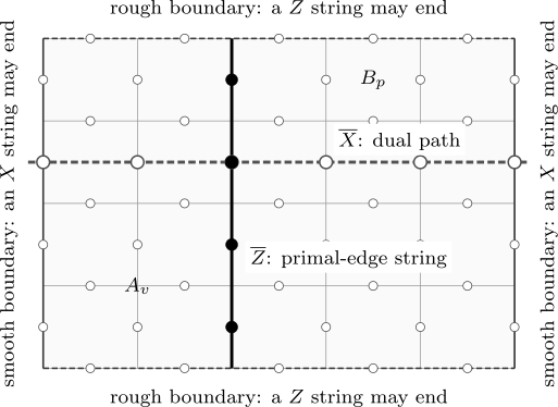
Schematic edge-qubit patch. The solid $\overline Z$ string joins rough boundaries; the dashed dual path marks the support of $\overline X$ joining smooth boundaries. Their single shared data qubit gives the required anticommutation. The highlighted $A_v$ and $B_p$ indicate representative local checks, not a complete syndrome-extraction circuit.

Distance

The code distance is

$$d = \min_{P\in N(S)\setminus S} \operatorname{wt}(P),$$

where $S$ is the stabilizer group and $N(S)$ its Pauli normalizer. Geometrically, $d$ is the shortest undetectable nontrivial string, including paths that join compatible boundaries or encircle a defect.

A nominally wide patch can still have small distance if one boundary neck is narrow, if a hole approaches another boundary, or if a circuit-level correlated fault creates a dangerous short logical path. Distance is a property of the complete code and extraction schedule, not the visual area alone.

Holes, punctures, and defects

Turning off a connected set of checks creates a puncture whose boundary can condense one syndrome type. Logical information may then be represented by a loop around a hole and a conjugate string joining that hole to another compatible boundary or defect. Moving or resizing holes by changing which checks are measured is code deformation.

Holes are useful for routing and logical operations, but each deformation must preserve a minimum spacetime distance. A large geometric separation at one instant does not protect against a short fault path created during the motion.

Rotated Planar Patches

The rotated planar code redraws the same CSS incidence structure so that a one-logical-qubit distance-$d$ patch can use fewer data qubits. For the common odd-$d$ square patch:

$$n_{\mathrm{data}} = d^2, \qquad n_{\mathrm{checks}} = d^2-1.$$

The independent checks divide evenly:

$$n_X = n_Z = \frac{d^2-1}{2}.$$

If every check has a dedicated measurement ancilla, the idealized patch contains

$$n_{\mathrm{data+ancilla}} = 2d^2-1$$

qubits before adding routing, couplers, spare qubits, flag or leakage-removal ancillas, and control hardware. By comparison, a common unrotated distance-$d$ planar layout uses

$$n_{\mathrm{data}} = d^2+(d-1)^2.$$

These formulas are layout counts, not universal resource estimates.

For example, an idealized rotated distance-5 patch has 25 data qubits and 24 check ancillas, for 49 qubits under the one-ancilla-per-check convention. Its abstract distance permits correction of every data-qubit Pauli error of weight

$$t = \left\lfloor\frac{d-1}{2}\right\rfloor = 2.$$

That statement does not mean every pair of circuit faults is corrected. Propagated ancilla faults, measurement faults, leakage, and boundary-time effects must be included in the circuit-level distance.

Syndrome Extraction

Star–plaquette scheduling

An edge-data layout assigns each star and plaquette check a measurement ancilla, but the local check definitions do not yet determine a circuit schedule. A complete round must place every incident data–ancilla interaction into time steps such that no qubit participates in two gates at once. It must also declare preparation, reset, readout, idle locations, and any boundary check whose weight is reduced. The result is a global star–plaquette schedule, not merely a collection of independent weight-four parity circuits.

Different valid schedules can implement the same ideal stabilizers while producing different correlated errors under a single circuit fault. The chronological order around each star or plaquette fixes which pairs of data qubits can inherit an ancilla fault. Neighboring orders therefore have to be chosen together, including the truncated checks at rough and smooth boundaries.

Hook orientation and spacetime history

A correlated two-data hook is a short chain segment. Its orientation matters because a sequence of aligned hooks can create a nontrivial string using fewer faults than the nominal code distance suggests. A surface-code schedule is audited by comparing every allowed hook with the patch’s logical string directions and boundaries. The safe ordering depends on whether the check is star or plaquette, on the patch convention, and on which logical operator a boundary can terminate; there is no code-independent clockwise ordering rule.

Repeated rounds turn the scheduled patch into a spacetime object. In the bulk, a data-chain segment has endpoints on neighboring checks, while a transient readout fault commonly produces time-separated violations at one check. Spatial boundaries permit some chains to terminate, and temporal boundaries permit endpoints to pair with preparation or final-data parity relations. A surface-code detector graph must encode those boundary attachments, the actual gate schedule, and known frame offsets. Omitting them can reduce the circuit-level distance even when the static patch distance is unchanged.

Circuit-level hazards

Repeated extraction brings several physical mechanisms into the code:

• ancilla preparation and measurement errors;
• two-qubit-gate propagation and hook orientation;
• data-idle errors during a schedule;
• crosstalk and coherent calibration drift;
• leakage outside the computational subspace;
• reset failure and delayed leakage removal;
• long-range bursts and time-correlated faults;
• classical latency or dropped syndrome data.

A code-capacity model that places independent Pauli errors only on data qubits is useful for theory, but it cannot by itself predict circuit-level hardware performance.

Decoding the Syndrome History

Recovery as an equivalence-class decision

Suppose the actual data error is $E$ and a decoder chooses a Pauli recovery $C$ with the same syndrome. Then $CE$ has zero syndrome and lies in the normalizer. Recovery succeeds when

$$CE\in S,$$

and fails logically when

$$CE\in N(S)\setminus S.$$

The decoder does not need to reconstruct $E$ exactly. It needs the correct logical equivalence class modulo stabilizers. This distinction is central because many microscopic chains share the same boundary and act identically on the code space.

In practice, $C$ is usually not applied as a layer of physical Pauli gates. The controller updates a Pauli frame and reinterprets later measurements or adapts later Clifford operations. Avoiding unnecessary corrections prevents additional gate faults.

Minimum-weight perfect matching

For sparse stochastic faults, detection events often appear in pairs or connect to allowed boundaries. A matching decoder constructs a graph whose vertices are detection events. An edge represents a candidate fault chain joining two events or joining an event to a boundary.

The minimum-weight perfect matching section derives calibrated log-odds weights and distinguishes a most likely path from a most likely logical class. In the surface-code graph, matching pairs every detection event, possibly to a boundary, and the associated paths define a recovery class.

Several qualifications matter:

• shortest geometric distance is appropriate only for a sufficiently uniform noise model;
• circuit faults can create diagonal, time-like, or correlated graph edges;
• $X$ and $Z$ matching graphs treated separately can miss $Y$ correlations;
• degeneracy means many chains can realize the same logical class;
• an exact maximum-likelihood decoder compares sums of probabilities over equivalence classes, not only the single most likely chain;
• real-time operation imposes latency, memory, and throughput constraints absent from an offline benchmark.

Matching is therefore an important decoder, not a definition of the surface code. The decoder comparison places union–find, tensor-network, renormalization, belief-propagation with ordered-statistics postprocessing, correlated matching, and learned decoders on their different accuracy–latency–hardware tradeoffs.

A one-dimensional decoding analogy

Suppose two $X$-check detection events are separated by three lattice edges. A decoder may infer a length-3 $Z$ chain joining them. Another chain with the same endpoints that differs by a plaquette boundary is stabilizer-equivalent and equally safe. A competing chain that reaches rough boundaries can differ by $\overline Z$ and cause a logical error.

The syndrome fixes the endpoints, not which homology class produced them. Increasing $d$ makes the shortest wrong-class explanation longer, which is the geometric origin of error suppression below threshold.

Thresholds Without a Universal Number

Operational meaning

Consider a family of increasing distances with the same local architecture, noise model, extraction protocol, decoder, and logical-error metric. A threshold $p_{\mathrm{th}}$ separates two scaling regimes:

• for $p<p_{\mathrm{th}}$, increasing $d$ suppresses the logical error rate;
• for $p>p_{\mathrm{th}}$, increasing $d$ does not provide asymptotic suppression.

The threshold is therefore a property of the complete family and contract. Code-capacity noise, phenomenological measurement noise, depolarizing circuit noise, biased noise, erasures, leakage, and correlated noise generally produce different values. Decoder choice changes the value as well.

Useful fit and its limits

For odd distances in a sufficiently low-error regime, simulation data are often summarized by

$$p_{\mathrm L}(p,d) \approx A \left( \frac{p}{p_{\mathrm{th}}} \right)^{(d+1)/2},$$

where $A$ and $p_{\mathrm{th}}$ are fit parameters for a specified experiment. The exponent reflects the leading number of faults needed to defeat a distance-$d$ fault-tolerant construction.

This formula is not a theorem, and it is not reliable arbitrarily close to threshold, at very small $d$, under strongly correlated noise, or when different fault mechanisms dominate different distances. A serious scaling claim reports uncertainty, fit range, rounds, decoder, leakage treatment, and the definition of $p_{\mathrm L}$.

Pseudothreshold and finite-size crossings

A pseudothreshold is a finite-size comparison, often the physical error rate at which a particular encoded circuit performs as well as a chosen unencoded reference. Curves for distances $d$ and $d+2$ may also cross near a finite-size estimate of the asymptotic threshold. Neither quantity is automatically the constant in the Threshold Theorem, which first fixes the code, gadgets, architecture, noise class, and metric.

Logical error per cycle, logical failure after $d$ rounds, logical parity-measurement error, and logical CNOT error are different metrics. Quoting one as though it described every operation obscures the architecture.

What scaling evidence establishes

Observing

$$p_{\mathrm L}(d+2)<p_{\mathrm L}(d)$$

under matched conditions is direct evidence that the tested system operates in a below-threshold scaling regime for that metric and distance range. It does not by itself establish:

• arbitrarily low logical error;
• a universal threshold;
• fault-tolerant non-Clifford gates;
• scalable classical decoding;
• acceptable fabrication yield or cryogenic control;
• an application-level resource advantage.

Experiments have nevertheless made this hierarchy measurable. Repeated surface-code detection, distance scaling, leakage handling, and logical operations test distinct layers of the fault-tolerance stack and should be reported as such.

Lattice Surgery

Lattice surgery performs logical operations by temporarily changing stabilizer measurements along adjacent patch boundaries. A merge introduces joint checks spanning two patches; a split restores separate boundaries. Repeating the new checks for enough rounds protects the parity result against measurement faults.

The essential operation is a joint logical Pauli measurement such as

$$M_{ZZ} = \overline Z_1\overline Z_2$$

or

$$M_{XX} = \overline X_1\overline X_2.$$

The outcome reveals only a parity. It does not reveal the individual eigenvalues of $\overline Z_1$ and $\overline Z_2$. For example, the $+1$ eigenspace of $M_{ZZ}$ contains both logical basis states $|0_L0_L\rangle$ and $|1_L1_L\rangle$, so a parity measurement can preserve coherent superpositions within that subspace.

A logical CNOT can be built, up to tracked Pauli corrections, using an ancilla patch prepared in $|+_L\rangle$, a joint $\overline Z\overline Z$ measurement between control and ancilla, a joint $\overline X\overline X$ measurement between ancilla and target, and a final logical-$Z$ measurement of the ancilla. Classical feed-forward determines the Pauli-frame updates.

The geometric operation is not instantaneous. To maintain distance $d$, a merge, split, or boundary move typically occupies $O(d)$ syndrome rounds and $O(d^2)$ qubit area. Exact constants depend on layout, routing, check schedule, and whether neighboring operations can be packed in parallel. Fault-Tolerant Gates places surgery inside the general error-containment contract. Lattice Surgery owns the patch conventions, protected parity protocols, correction tables, and scheduling details; the canonical surface-code principle here is the protected measurement of joint logical parity.

Resource Overhead

Space, time, and spacetime volume

A one-qubit rotated patch uses $O(d^2)$ data and measurement qubits. A protected measurement or deformation typically lasts $O(d)$ code cycles. The natural leading resource for an operation is therefore a spacetime volume of order

$$O(d^3),$$

before constant factors and parallel scheduling are included.

This scaling alone does not determine a machine size. A resource estimate must allocate:

• logical data patches;
• routing and temporary ancilla patches;
• magic-state distillation or cultivation factories;
• storage buffers and communication lanes;
• decoder hardware and classical reaction time;
• physical qubits unavailable because of defects or yield;
• calibration, reset, leakage-removal, and readout resources;
• an error budget divided among all logical operations.

For many algorithms, non-Clifford state factories dominate the footprint. For others, data storage, routing congestion, or a slow measurement cycle dominates. Reporting only $2d^2-1$ qubits per patch can therefore understate total resources by a large architecture-dependent factor.

Choosing distance

Distance should be selected from an error budget, not from a slogan. If a computation uses $N_{\mathrm{loc}}$ logical locations and the allowed total failure probability is $\epsilon$, a first union-bound allocation might require

$$p_{\mathrm L} \lesssim \frac{\epsilon}{N_{\mathrm{loc}}}.$$

One then uses measured or simulated logical scaling under the intended architecture to choose $d$. Different operations may justify different distances, and optimized systems can allocate nonuniform error budgets. Extrapolation beyond validated distances must be labeled as a model prediction.

Hardware Relevance

The surface code trades qubit efficiency for locality and repeated measurement. Its bounded-weight checks align naturally with platforms offering a two-dimensional coupling graph, fast mid-circuit readout, reset, and stable repeated gates. Those advantages explain its central role in superconducting-qubit roadmaps and its broader use as an architectural benchmark.

The code does not make local hardware imperfections irrelevant. Several effects are particularly consequential:

• leakage: a leaked qubit can corrupt several later checks until it is reset or replaced;
• correlated faults: crosstalk, shared control, radiation events, and bursts can defeat independent-edge decoders;
• coherent errors: systematic rotations need not behave like stochastic Pauli faults at short times;
• measurement latency: slow readout lengthens data-idle exposure and decoder deadlines;
• connectivity defects: disabled qubits and couplers reshape checks and shorten paths unless the patch is adapted;
• calibration drift: decoder weights and circuit error models can become stale;
• classical backlog: a decoder that is accurate but slower than syndrome production is not operationally scalable.

The surface code is an actively corrected topological code, not a self-correcting memory at nonzero temperature. Without repeated syndrome extraction and energy-consuming feedback or frame tracking, thermally or environmentally generated error strings can grow and become logical. Topological language describes the nonlocal equivalence classes; it does not supply passive lifetime growth by itself.

Variants and Naming

Several related constructions share the surface-code idea:

Variant	Distinguishing feature
toric code	periodic boundaries and two logical qubits on a torus
unrotated planar code	open patch in the original edge-qubit geometry
rotated planar code	reduced data-qubit count for a common square one-qubit patch
defect or hole encoding	punctures support loop and connecting-string logicals
twist-based layout	boundary-type changes and twists alter logical-string endpoints
XZZX surface code	locally transformed check pattern useful under certain biased-noise contracts
subsystem surface code	gauge measurements replace some direct stabilizer measurements

These names do not remove the need for a circuit and decoder specification. In particular, a favorable threshold for one variant under tailored biased noise should not be transferred to a different device model.

Common Mistakes

• Treating “surface code” and “toric code” as exact synonyms.
• Defining rough and smooth boundaries by appearance instead of stating which Pauli strings may terminate.
• Counting geometric width as distance without checking every logical path and the extraction circuit.
• Inferring the microscopic error chain uniquely from its syndrome endpoints.
• Applying physical corrections after every round when a Pauli frame suffices.
• Quoting a threshold without the noise model, schedule, decoder, and metric.
• Calling a finite-size pseudothreshold an asymptotic threshold.
• Counting only data qubits while omitting check ancillas, routing, factories, and classical decoding.
• Describing active topological error correction as passive self-correction.
• Assuming independent CSS matching captures leakage, $Y$ correlations, and burst errors automatically.

Exercises

1. Star–plaquette commutation

Prove that an edge-qubit star $A_v$ commutes with every plaquette $B_p$ on the square lattice.

Solution

If $v$ is not a corner of $p$, the operators have disjoint support and commute. If $v$ is a corner of $p$, the star and plaquette share the two boundary edges meeting at that corner. On each shared qubit, $X$ anticommutes with $Z$, producing a factor $-1$. The two factors cancel:

$$A_vB_p = (-1)^2B_pA_v = B_pA_v.$$

Thus every $X$-type and $Z$-type generator has even support overlap.

2. Encoded qubits on a torus

Use stabilizer counting and Euler’s relation to show that the edge-qubit toric code encodes two qubits.

Solution

There are $n=E$ data qubits. There are $V+F$ nominal checks, but the product of all stars and the product of all plaquettes are identities, leaving rank

$$r = V+F-2.$$

The number of encoded qubits is

$$\begin{aligned} k &= n-r \\ &= E-V-F+2. \end{aligned}$$

Euler’s relation $V-E+F=0$ on the torus gives $E-V-F=0$, hence $k=2$.

3. Why a logical string has no syndrome

Explain why a $Z$ string connecting two rough boundaries commutes with every measured stabilizer but is not generally a stabilizer.

Solution

Every bulk vertex along the path touches zero or two supported edges, so the string commutes with every star check. Its two endpoints lie on boundaries where $Z$ strings are permitted to terminate, so no endpoint syndrome is measured there. It also commutes with all plaquette checks because both contain only $Z$ operators.

The string cannot generally be contracted to a product of local plaquette boundaries while keeping its endpoints on the same boundary. It joins distinct rough boundaries and represents a nontrivial relative homology class. Therefore it lies in $N(S)\setminus S$ and acts as $\overline Z$.

4. A distance-5 rotated patch

For the common odd-distance rotated patch with one dedicated ancilla per check, find the number of data qubits, check ancillas, total patch qubits, and guaranteed correctable data-error weight at $d=5$.

Solution

The layout formulas give

$$n_{\mathrm{data}} = d^2 = 25,$$

and

$$n_{\mathrm{checks}} = d^2-1 = 24.$$

With one ancilla per check, the idealized total is $25+24=49$ qubits. The abstract distance guarantees correction of all data Pauli errors of weight at most

$$t = \left\lfloor \frac{d-1}{2} \right\rfloor = 2.$$

This count excludes routing, spare qubits, leakage-removal resources, and circuit-level correlated faults.

5. One faulty check measurement

Suppose the true stabilizer eigenvalue is constant and equal to $+1$, but round $t$ reports $m_a(t)=-1$ while rounds $t-1$ and $t+1$ report $+1$. Locate the detection events.

Solution

By definition,

$$\delta_a(t) = m_a(t)m_a(t-1) = -1,$$

and

$$\delta_a(t+1) = m_a(t+1)m_a(t) = -1.$$

The single measurement fault therefore produces two time-separated detection events at the same spatial check location. This is represented by a time-like edge in the decoding graph.

6. Same syndrome, successful recovery

Let $E$ be the actual error and $C$ a decoder’s correction with the same syndrome. Why is $CE\in S$ the success condition rather than $C=E$?

Solution

Equal syndromes imply that $CE$ has zero syndrome and preserves the code space. Stabilizers act as the identity on every encoded state, so if $CE\in S$ then

$$C E|\psi_L\rangle = |\psi_L\rangle$$

for every code state. The microscopic chains $C$ and $E$ may differ while having the same logical action. If instead $CE\in N(S)\setminus S$, their difference is a nontrivial logical Pauli and recovery fails.

7. Audit a threshold claim

A report states, “The surface-code threshold is $1\%$.” List at least five missing pieces needed to interpret the claim.

Solution

The report should specify at least:

• the code variant and boundary layout;
• whether noise is code-capacity, phenomenological, or circuit-level;
• the probabilities assigned to gates, idles, reset, and measurement;
• whether leakage and correlations are included;
• the check-extraction schedule and number of rounds;
• the decoder and its weighting model;
• the logical-error metric;
• the distance range and finite-size fitting procedure.

Without this contract, the number cannot be transferred to another architecture.

8. Joint parity without individual readout

Show that measuring $\overline Z_1\overline Z_2$ does not reveal the individual logical $Z$ values.

Solution

The $+1$ parity subspace is spanned by

$$|0_L0_L\rangle, \qquad |1_L1_L\rangle,$$

while the $-1$ parity subspace is spanned by

$$|0_L1_L\rangle, \qquad |1_L0_L\rangle.$$

Each outcome leaves two possible individual value pairs. Moreover, a coherent state such as

$$\alpha|0_L0_L\rangle + \beta|1_L1_L\rangle$$

remains coherent after obtaining parity $+1$. The measurement reveals only the product eigenvalue.

9. Why a Pauli frame helps

Explain why a decoder can record a correction instead of immediately applying physical Pauli gates.

Solution

Pauli corrections can be propagated through later Clifford gates by conjugation and absorbed into the interpretation of later measurements. The controller therefore records the accumulated logical and physical Pauli frame. This produces the same logical statistics as applying the gates, while avoiding extra faulty control operations. A non-Clifford operation or adaptive measurement may require the frame to influence later control, but it still need not be realized as an immediate physical Pauli pulse.

10. Active versus self-correcting protection

Why does nonlocal logical information not make a two-dimensional surface-code memory passively self-correcting?

Solution

Nontrivial logical strings are extended, but local errors can build such a string one segment at a time without an energy barrier that grows with system size in the ordinary two-dimensional toric-code setting. At nonzero temperature or under continuing environmental noise, faults therefore accumulate. Repeated parity measurements, decoding, and frame updates are needed to remove them before they form a logical class. The code is topological and actively corrected, not a passive memory whose lifetime diverges solely because the patch is larger.

Further Connections

• Why Quantum Error Correction Is Possible
• Stabilizer Formalism
• Color Codes owns the neighboring three-colored face-check geometry and transversal-Clifford structure; this page retains primal and dual strings, rough and smooth boundaries, extraction, detector graphs, matching, thresholds, surgery, and overhead.
• Error-Correction Case Studies compares repetition-code records, finite-distance surface-code memories, logical-lifetime references, and bosonic break-even evidence.
• Stabilizer Simulation develops repeated-round detector generation, batched Pauli-fault sampling, decoder isolation, logical-failure scoring, and threshold-experiment validation.
• Superconducting Qubits
• Common Noise Models
• Quantum Software Stack places code cycles, decoder deadlines, logical operations, factories, and failure budgets inside fault-tolerant lowering.
• Resource Estimation maps logical locations, code-distance fits, patch liveness, factory flow, routing, and cycle time into qubit, runtime, failure, and spacetime ledgers.
• Resource Estimation Tools develops the versioned software workflow for evaluating and validating those scenarios.
• Topological Order Preview
• Topological Order
• Anyons and Braiding
• Topological Quantum Computation Bridge
• Surface Code model card
• Stabilizer Identities
• Quantum Information Roadmap

References

• A. Y. Kitaev, “Fault-tolerant quantum computation by anyons,” Annals of Physics 303, 2–30, 2003, doi:10.1016/S0003-4916(02)00018-0.
• E. Dennis, A. Kitaev, A. Landahl, and J. Preskill, “Topological quantum memory,” Journal of Mathematical Physics 43, 4452–4505, 2002, doi:10.1063/1.1499754.
• S. B. Bravyi and A. Y. Kitaev, “Quantum codes on a lattice with boundary,” 1998, arXiv:quant-ph/9811052.
• A. G. Fowler, M. Mariantoni, J. M. Martinis, and A. N. Cleland, “Surface codes: Towards practical large-scale quantum computation,” Physical Review A 86, 032324, 2012, doi:10.1103/PhysRevA.86.032324.
• D. Horsman, A. G. Fowler, S. Devitt, and R. Van Meter, “Surface code quantum computing by lattice surgery,” New Journal of Physics 14, 123011, 2012, doi:10.1088/1367-2630/14/12/123011.
• A. M. Stephens, “Fault-tolerant thresholds for quantum error correction with the surface code,” Physical Review A 89, 022321, 2014, doi:10.1103/PhysRevA.89.022321.
• B. M. Terhal, “Quantum error correction for quantum memories,” Reviews of Modern Physics 87, 307–346, 2015, doi:10.1103/RevModPhys.87.307.
• D. S. Wang, A. G. Fowler, and L. C. L. Hollenberg, “Surface code quantum computing with error rates over 1%,” Physical Review A 83, 020302(R), 2011, doi:10.1103/PhysRevA.83.020302.
• D. Litinski, “A game of surface codes: Large-scale quantum computing with lattice surgery,” Quantum 3, 128, 2019, doi:10.22331/q-2019-03-05-128.
• J. P. Bonilla Ataides, D. K. Tuckett, S. D. Bartlett, S. T. Flammia, and B. J. Brown, “The XZZX surface code,” Nature Communications 12, 2172, 2021, doi:10.1038/s41467-021-22274-1.
• N. Delfosse and N. H. Nickerson, “Almost-linear time decoding algorithm for topological codes,” Quantum 5, 595, 2021, doi:10.22331/q-2021-12-02-595.
• Google Quantum AI and Collaborators, “Suppressing quantum errors by scaling a surface code logical qubit,” Nature 614, 676–681, 2023, doi:10.1038/s41586-022-05434-1.
• Google Quantum AI and Collaborators, “Quantum error correction below the surface code threshold,” Nature 638, 920–926, 2025, doi:10.1038/s41586-024-08449-y.

Summary

The surface code converts local parity information into protection of nonlocal logical strings. In the edge-qubit picture, commuting star and plaquette checks detect the endpoints of $Z$ and $X$ error chains. Boundaries determine which strings may terminate, and code distance is the shortest nontrivial logical representative.

Real protection comes from repeated, fault-tolerant syndrome extraction and spacetime decoding. A decoder must choose the correct equivalence class, not reconstruct the exact microscopic error. Thresholds, scaling laws, and overhead are meaningful only after fixing the complete architecture contract. Lattice surgery then turns protected boundary-parity measurements into logical operations, while the physical machine must still manage leakage, correlations, decoding latency, routing, and non-Clifford resources.