Common Noise Models

Short Definition

A noise model is a declared mathematical approximation to how an implemented quantum process differs from its target. A useful model specifies the system boundary, basis, parameter convention, time step, circuit context, correlations, and observables it is expected to predict.

This page is a device- and circuit-facing reference for:

• Pauli and depolarizing noise;
• dephasing and phase-damping conventions;
• amplitude damping and finite-temperature relaxation;
• erasure, loss, leakage, and seepage;
• coherent overrotation;
• spatially and temporally correlated noise.

The formulas below are model cards, not microscopic derivations. Common Noise Channels and its linked pages own the general channel theory, Kraus constructions, Choi tests, dilations, and master-equation limits. Noise in Quantum Information owns the broader taxonomy and diagnostic workflow.

Noise, Channels, and Error Mitigation owns the decision and evidence ledger used to choose or reject a model; this page retains explicit device-facing model cards, parameter conversions, composition rules, and falsification checks.

Quantum Channels for QI owns convention-complete representation translation and invariant checks; this page retains model cards, parameter conventions, placement rules, and falsifiers.

Pauli Noise and Depolarizing Channels owns detailed Pauli-probability and transfer-eigenvalue composition, Clifford and stabilizer propagation, syndrome and logical pushforwards, and the depolarizing-approximation audit; this page retains compact cross-model cards, parameter lookup, placement rules, and falsifiers.

Dephasing and Amplitude Damping owns the protocol-qualified T1–T2 and equilibrium-population conversion, finite thermal channel, physicality, composition, and held-out adequacy workflow; this page retains compact cross-model cards, parameter lookup, placement rules, and falsifiers.

Leakage and Crosstalk owns the full-space and survival-branch crosswalk, state and average leakage/seepage/coherence metrics, leakage flags, scalar population licenses, operational crosstalk tests, and context-aware composition; this page retains compact cross-model cards, parameter lookup, placement rules, and first-line falsifiers.

The Threshold Theorem owns the locality and fault-tail assumptions needed to turn such models into an asymptotic fault-tolerance claim.

A Model Is More Than a Formula

Two software packages can use the phrase “depolarizing probability $p$” for different channels. Two experiments can have the same average infidelity while one is dominated by stochastic Pauli faults and the other by coherent overrotation. A channel fitted to isolated gates can fail under simultaneous gates or after calibration drift.

Every model card should record:

1. system: qubit, qudit, bosonic mode, code subspace, or enlarged physical space;
2. basis: computational, energy, measurement, instantaneous eigenbasis, or another declared basis;
3. map: channel, trace-decreasing branch, unitary offset, stochastic process, or correlated sequence;
4. parameters: definitions, ranges, units, and identity limit;
5. time step: gate duration, idle interval, correction cycle, or continuous-time rate;
6. composition order: where the model is inserted relative to gates, idles, reset, and measurement;
7. context: qubits, simultaneous operations, pulse schedule, temperature, and calibration epoch;
8. correlations: independence assumptions across qubits, locations, and shots;
9. validation: circuits and observables not used to fit the parameters.

Without these fields, a compact noise model is not reproducible.

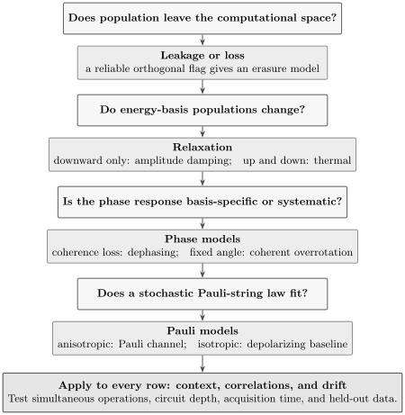
A practical model-selection map. Each row asks what structure the data and hardware retain. The rows are not mutually exclusive: a device model may combine amplitude damping, pure dephasing, leakage, coherent control error, and correlated context dependence. Correlations and drift can modify every named channel.

Quick Lookup

Model	Identity limit	Core action	Deliberately omitted structure
Pauli channel	$p_I=1$	random Pauli-string conjugation	nonunital damping and coherent phase
depolarizing	shrink factor $1$	isotropic contraction	preferred axes and microscopic mechanism
dephasing	coherence factor $\lambda=1$	transverse coherence contraction	energy relaxation
amplitude damping	$\gamma=0$	downward population transfer	thermal excitation
thermal relaxation	$\gamma=0$	relaxation toward finite-temperature fixed state	extra pure dephasing
erasure	$\epsilon=0$	orthogonally flagged loss	unflagged loss mechanism
leakage model	leakage rate $\ell=0$	population leaves computational subspace	full leaked-state dynamics unless added
coherent overrotation	$\epsilon=0$	systematic unitary displacement	stochastic variation unless added
correlated model	factorized joint law	joint or history-dependent faults	no universal omitted structure

The identity limit is a useful implementation test. Setting the listed error parameters to their identity values should reproduce the target process, including its output Hilbert space and classical flags.

Pauli Channels

For $n$ qubits, let $\mathcal P_n$ denote Pauli strings with global phases omitted. A stochastic Pauli channel is

$$\begin{aligned} \mathcal E_{\mathrm P}(\rho) &= \sum_{P\in\mathcal P_n} p_P\,P\rho P, \\ p_P &\geq0, \qquad \sum_Pp_P=1. \end{aligned}$$

The probability $p_I$ is the no-Pauli-fault probability for this model step. A one-qubit channel is

$$\begin{aligned} \mathcal E_{\mathrm P}(\rho) &= p_I\rho + p_X\,X\rho X \\ &\quad+ p_Y\,Y\rho Y + p_Z\,Z\rho Z. \end{aligned}$$

Pauli channels are convenient because stabilizer propagation, syndrome probabilities, and many decoder models become classical probability calculations. They are unital and diagonal in the Pauli operator basis.

That convenience is also the boundary:

• amplitude damping is nonunital and is not a Pauli channel;
• leakage changes the modeled subspace;
• a fixed overrotation is coherent, not a random Pauli event;
• a multiqubit Pauli distribution can be correlated even though every term is a Pauli string.

An independent Pauli model requires the joint probabilities to factorize over qubits or locations. Merely writing a Pauli channel does not imply independence. Pauli Channels gives the canonical Bloch eigenvalues and complete-positivity conditions.

Depolarizing Noise and Its Conventions

The depolarizing model removes directional structure. For a qubit, one common replacement convention is

$$\mathcal D_q^{\mathrm{rep}}(\rho) = (1-q)\rho + q\frac{I}{2}, \qquad 0\leq q\leq1.$$

The Bloch vector shrinks as

$$\mathbf r \longmapsto (1-q)\mathbf r.$$

Another common total Pauli-error convention is

$$\begin{aligned} \mathcal D_p^{\mathrm{Pauli}}(\rho) &= (1-p)\rho \\ &\quad+ \frac p3 \left( X\rho X+Y\rho Y+Z\rho Z \right), \\ 0 &\leq p\leq1. \end{aligned}$$

Its Bloch shrink factor is

$$\lambda = 1-\frac{4p}{3}.$$

Where both parameterizations describe the same channel,

$$q = \frac{4p}{3}, \qquad p = \frac{3q}{4}.$$

The replacement interpretation restricts $0\leq q\leq1$, corresponding to $0\leq p\leq3/4$. The Pauli mixture remains a valid channel up to $p=1$, where $\lambda=-1/3$ and $q=4/3$ is no longer a literal replacement probability.

For the identity target, the one-qubit average infidelity is

$$r = 1-F_{\mathrm{avg}} = \frac q2 = \frac{2p}{3}.$$

Thus the phrases “depolarizing probability,” “Pauli error probability,” “Bloch shrink,” and “average infidelity” name different numbers. Always convert through the channel action. Depolarizing Channel owns the $d$-dimensional family and complete-positivity range.

Depolarizing noise is appropriate as:

• a symmetry-reduced benchmark model;
• a controlled toy model;
• an effective model after justified randomization or twirling;
• a baseline against which structured models are compared.

It is rarely a complete microscopic device model.

Dephasing and Phase Damping

Choose a preferred qubit basis. A robust convention uses the coherence factor $\lambda$:

$$\begin{aligned} \rho_{00}'&=\rho_{00}, & \rho_{11}'&=\rho_{11}, \\ \rho_{01}'&=\lambda\rho_{01}, & \rho_{10}'&=\lambda^*\rho_{10}, \\ |\lambda|&\leq1. \end{aligned}$$

If $\lambda=|\lambda|e^{-i\theta}$, the magnitude describes coherence loss and $\theta$ is a coherent $Z$ rotation. For real $\lambda$, the equivalent phase-flip mixture is

$$\begin{aligned} \Phi_{p_Z}(\rho) &= (1-p_Z)\rho + p_Z\,Z\rho Z, \\ \lambda &= 1-2p_Z. \end{aligned}$$

Therefore

$$p_Z = \frac{1-\lambda}{2}.$$

The labels dephasing, phase damping, and phase-flip probability are not parameter conventions. For example, an API may define a strength $g$ through

$$\lambda=\sqrt{1-g}.$$

Only under that explicit definition is $g=1-\lambda^2$. Another source may call $1-\lambda$ or $(1-\lambda)/2$ its error probability. Record the matrix action when translating between tools.

The basis is part of the model. Pure dephasing in the energy basis preserves energy populations; the same map written in another basis need not look population preserving. Dephasing Channel owns the Kraus, Bloch-sphere, and master-equation treatments.

Amplitude Damping

Zero-temperature amplitude damping models relaxation from $|1\rangle$ to $|0\rangle$. With decay probability $\gamma$,

$$\begin{aligned} \rho_{00}' &= \rho_{00}+\gamma\rho_{11}, \\ \rho_{11}' &= (1-\gamma)\rho_{11}, \\ \rho_{01}' &= \sqrt{1-\gamma}\,\rho_{01}, \qquad \rho_{10}'=(\rho_{01}')^*. \end{aligned}$$

For a Markovian idle interval $\Delta t$ with relaxation time $T_1$,

$$\gamma(\Delta t) = 1-e^{-\Delta t/T_1}.$$

This map is nonunital: it moves the maximally mixed state toward $|0\rangle\langle0|$. It is therefore not equivalent to a Pauli or depolarizing channel with a matched average infidelity.

Use amplitude damping only when upward thermal excitation is negligible on the modeled timescale. Amplitude-Damping Channel owns the Kraus operators, dilation, Choi matrix, and zero-temperature master equation.

Combining T1 and T2 Without Double Counting

Suppose measured exponential times satisfy

$$\frac1{T_2} = \frac1{2T_1} + \frac1{T_\phi}.$$

Amplitude damping already multiplies coherence by

$$\sqrt{1-\gamma} = e^{-\Delta t/(2T_1)}.$$

The additional pure-dephasing factor should therefore be

$$\lambda_\phi = e^{-\Delta t/T_\phi}, \qquad \frac1{T_\phi} = \frac1{T_2} - \frac1{2T_1}.$$

The combined transverse factor is

$$\sqrt{1-\gamma}\,\lambda_\phi = e^{-\Delta t/T_2}.$$

A common mistake is to compose amplitude damping with a dephasing channel whose factor is already $e^{-\Delta t/T_2}$. That counts the $T_1$ contribution twice.

This construction assumes matched exponential, Markovian, two-level data at the same operating point. Ramsey $T_2^\ast$, echo $T_2$, drive-dependent decay, nonexponential envelopes, and leakage require a more explicit model.

Finite-Temperature Relaxation

When the bath can both excite and relax a qubit, use upward and downward rates $\Gamma_\uparrow$ and $\Gamma_\downarrow$. The equilibrium excited-state population is

$$n_{\mathrm{eq}} = \frac{\Gamma_\uparrow} {\Gamma_\uparrow+\Gamma_\downarrow}.$$

For a Markovian interval $\Delta t$, define

$$\gamma_T = 1- \exp\left[ -(\Gamma_\uparrow+\Gamma_\downarrow)\Delta t \right].$$

The thermal-relaxation model card can be written directly as

$$\begin{aligned} \rho_{11}' &= (1-\gamma_T)\rho_{11} + \gamma_T n_{\mathrm{eq}}, \\ \rho_{01}' &= \sqrt{1-\gamma_T}\,\rho_{01}, \end{aligned}$$

before adding any independent pure dephasing. The fixed state has excited population $n_{\mathrm{eq}}$. The zero-temperature amplitude-damping limit is $n_{\mathrm{eq}}=0$.

For a thermal bath and level spacing $\hbar\omega$, detailed balance gives

$$\frac{\Gamma_\uparrow}{\Gamma_\downarrow} = e^{-\beta\hbar\omega}.$$

Thermal Master Equations and Detailed Balance own the physical derivation. A fitted equilibrium population is not by itself proof that the environment has one thermodynamic temperature.

Erasure and Flagged Loss

A flagged erasure channel enlarges the output space with an orthogonal state $|e\rangle$. For normalized input $\rho$,

$$\mathcal E_\epsilon(\rho) = (1-\epsilon)V\rho V^\dagger + \epsilon|e\rangle\langle e|,$$

where $V$ embeds the input into the surviving output subspace. The receiver can distinguish erasure from every valid surviving state.

This model is useful for located faults, heralded transmission failure, and codes that exploit known error positions. It is not interchangeable with:

• depolarization, where the damaged output remains unflagged in the system space;
• postselected survival, where failed runs are removed and success probability must be retained;
• bosonic attenuation, where photon loss need not create a reliable flag;
• detector inefficiency, where a no-click event may have several causes.

Erasure and Loss Channels owns these distinctions and the trace-decreasing survival branch.

Leakage and Seepage

Leakage transfers population between the computational subspace $\mathcal H_C$ and a leakage subspace $\mathcal H_L$. A qubit-only channel cannot represent this transfer while remaining trace preserving. The physical model must use

$$\mathcal H_{\mathrm{phys}} = \mathcal H_C \oplus \mathcal H_L$$

or include an explicit leakage flag.

A coarse population model for one step uses leakage probability $\ell$ and seepage probability $s$:

$$\begin{pmatrix} P_C'\\ P_L' \end{pmatrix} = \begin{pmatrix} 1-\ell&s\\ \ell&1-s \end{pmatrix} \begin{pmatrix} P_C\\ P_L \end{pmatrix}.$$

If $\ell+s>0$, its stationary leakage population is

$$P_L^{(\infty)} = \frac{\ell}{\ell+s}.$$

This two-state Markov model tracks population only. A complete leakage model also specifies:

• coherent coupling between computational and leakage levels;
• operations and phases while leaked;
• how leaked states interact with neighbors;
• whether measurement resolves leakage;
• what state returns under seepage or reset.

Leakage reduction can lower $P_L$ without restoring the logical state. The computational projector and operational leakage metric are introduced in Noise in Quantum Information.

Coherent Overrotation

A fixed control error is often modeled by

$$\begin{aligned} \widetilde{\mathcal U}(\rho) &= V_\epsilon U\rho U^\dagger V_\epsilon^\dagger, \\ V_\epsilon &= \exp\left( -\frac{i\epsilon G}{2} \right). \end{aligned}$$

The placement of $V_\epsilon$ before or after $U$ matters unless the operators commute. The generator $G$, sign convention, and whether $\epsilon$ is fixed, slowly drifting, or independently sampled are part of the model.

If $\epsilon$ varies with density $f(\epsilon)$ and the value is unobserved, the averaged channel is

$$\overline{\mathcal V}(\rho) = \int d\epsilon\, f(\epsilon) V_\epsilon\rho V_\epsilon^\dagger.$$

For a fixed Pauli generator, symmetric phase averaging can resemble dephasing in that generator’s eigenbasis. A nonzero mean retains a coherent rotation. This does not justify replacing every calibration error by a Pauli or depolarizing channel.

Randomized compiling can tailor specified coherent errors into effective stochastic Pauli noise under its assumptions. The tailored model describes the randomized circuit ensemble, not the original bare circuit.

Correlated Noise

Correlations are structure in a joint distribution or process, not a separate single-qubit channel. An $n$-qubit Pauli model

$$\mathcal E(\rho) = \sum_{P\in\mathcal P_n} p_P\,P\rho P$$

is independent only when the relevant $p_P$ factorize. For example,

$$\begin{aligned} \mathcal E(\rho) ={}& (1-p_1-p_2-p_c)\rho \\ &+ p_1X_1\rho X_1 + p_2X_2\rho X_2 \\ &+ p_cX_1X_2\rho X_1X_2 \end{aligned}$$

contains an explicit two-qubit correlated fault. Its marginal error rates do not determine $p_c$.

A shared fluctuating field gives a different correlated model:

$$U(\theta) = \exp\left[ -\frac{i\theta}{2} \left( Z_1+Z_2 \right) \right],$$

followed by averaging over $\theta$. The resulting dephasing has collective structure and can preserve different subspaces than independent $Z$ noise.

Temporal correlations can be represented by a latent parameter sequence $\delta_k$ with autocovariance

$$C(m) = \mathbb E \left[ \delta_k\delta_{k+m} \right] - \mathbb E[\delta_k]\, \mathbb E[\delta_{k+m}].$$

Nonzero $C(m)$ rules out an independent sequence at that lag, but zero covariance does not prove full statistical independence. A memory model should state whether latent variables persist across gates, shots, resets, or calibration blocks.

Composition and Placement

For target gates $U_1,\ldots,U_L$, a simple gate-local model might be

$$\widetilde{\mathcal C} = \mathcal E_L \circ \mathcal U_L \circ\cdots\circ \mathcal E_1 \circ \mathcal U_1.$$

This notation already assumes that each $\mathcal E_j$ is a well-defined channel for that context and that no retained environment memory links the steps. Other placements, such as noise before the gate or during a simultaneous layer, can predict different results.

Composition order generally matters:

$$\mathcal E_2\circ\mathcal E_1 \neq \mathcal E_1\circ\mathcal E_2.$$

For example, a coherent rotation and nonunital damping need not commute. A compiler that reorders gates and idles also reorders their noise exposure.

State preparation and measurement belong at the boundaries:

$$p(y\mid x) = \operatorname{Tr} \left[ M_y\, \widetilde{\mathcal C} \left( \rho_x \right) \right].$$

Do not absorb every SPAM discrepancy into the gate channels unless the model is intentionally an end-to-end black box.

Markovian and Non-Markovian Noise owns the evidence required to promote finite channel cards to interval products, fixed-step powers, CP-divisible evolution, or a multitime model; this page retains explicit model formulas, parameter conventions, placement rules, and first-line adequacy tests.

Choosing the Smallest Useful Model

Use the simplest model that predicts held-out data at the required accuracy:

• Pauli model: stabilizer simulation, decoder studies, or data shown to be Pauli diagonal after tailoring.
• Depolarizing model: symmetric baseline, analytical estimate, or deliberately twirled benchmark.
• Amplitude damping plus pure dephasing: idle and gate-duration studies with matched exponential $T_1$ and $T_2$ data.
• Thermal relaxation: measurable upward transitions or non-negligible equilibrium excitation.
• Erasure: a reliable orthogonal flag or known fault location.
• Leakage model: multilevel occupation, atom loss, mode escape, or long-lived out-of-subspace population.
• Coherent unitary error: calibrated systematic angle, detuning, residual coupling, or phase offset.
• Correlated model: simultaneous-gate dependence, common-mode fluctuations, bursts, or memory across cycles.

Then try to falsify it. Compare isolated and simultaneous gates, several input axes, different depths, idle durations, qubit neighborhoods, and acquisition times. A larger model is justified when the residual structure matters for the target protocol, not merely because more parameters improve an in-sample fit.

Common Mistakes

• Using the symbol $p$ without defining the channel action.
• Equating depolarizing replacement probability, total Pauli probability, Bloch shrink, and average infidelity.
• Calling phase-flip probability a coherence-decay factor.
• Composing measured $T_2$ dephasing with amplitude damping and double counting the $T_1$ contribution.
• Using zero-temperature amplitude damping when upward transitions are visible.
• Treating erasure, postselection, leakage, and detector loss as the same event.
• Simulating leakage with a trace-preserving qubit channel.
• Assuming a multiqubit Pauli channel is independent.
• Replacing coherent error by stochastic noise without a physical averaging or tailoring procedure.
• Applying one stationary channel across context dependence or calibration drift.
• Validating a model only on the circuits used to fit it.

Exercises

1. Convert depolarizing conventions

A simulator uses the qubit replacement convention with $q=0.012$. Find the equivalent total nonidentity Pauli probability $p$, Bloch shrink factor $\lambda$, and average infidelity $r$.

Solution

The conversion is

$$p = \frac{3q}{4} = 0.009.$$

The Bloch shrink is

$$\lambda = 1-q = 0.988,$$

and the average infidelity is

$$r = \frac q2 = 0.006.$$

All four numbers describe the same qubit depolarizing channel under different conventions.

2. Translate dephasing parameters

A qubit channel leaves populations fixed and multiplies coherence by $\lambda=0.94$. Find the equivalent phase-flip probability $p_Z$. If another API defines phase-damping strength $g$ by $\lambda=\sqrt{1-g}$, find $g$.

Solution

The phase-flip probability is

$$p_Z = \frac{1-\lambda}{2} = 0.03.$$

For the explicitly stated second convention,

$$g = 1-\lambda^2 = 1-0.94^2 = 0.1164.$$

Neither $0.03$ nor $0.1164$ is “the” dephasing probability without its defining map.

3. Build a matched T1–T2 idle model

A qubit has $T_1=100\,\mu\mathrm{s}$ and exponential $T_2=80\,\mu\mathrm{s}$. For $\Delta t=1\,\mu\mathrm{s}$, compute $T_\phi$, amplitude-damping probability $\gamma$, and additional pure-dephasing factor $\lambda_\phi$. Verify the total coherence factor.

Solution

First,

$$\frac1{T_\phi} = \frac1{80} - \frac1{200} = \frac3{400} \,\mu\mathrm{s}^{-1},$$

so

$$T_\phi = \frac{400}{3}\,\mu\mathrm{s} \simeq 133.33\,\mu\mathrm{s}.$$

The damping probability is

$$\gamma = 1-e^{-1/100} \simeq 0.00995,$$

and

$$\lambda_\phi = e^{-1/T_\phi} = e^{-3/400} \simeq 0.99253.$$

Amplitude damping contributes $\sqrt{1-\gamma}=e^{-1/200}$. Therefore

$$\begin{aligned} \sqrt{1-\gamma}\,\lambda_\phi &= e^{-1/200}e^{-3/400} \\ &= e^{-1/80} \\ &\simeq 0.98758, \end{aligned}$$

which is the measured total $T_2$ factor.

4. Find a thermal fixed point

A qubit has $\Gamma_\uparrow=1\,\mathrm{kHz}$ and $\Gamma_\downarrow=9\,\mathrm{kHz}$. Find the equilibrium excited population. What value does zero-temperature amplitude damping incorrectly predict?

Solution

The thermal fixed population is

$$n_{\mathrm{eq}} = \frac{\Gamma_\uparrow} {\Gamma_\uparrow+\Gamma_\downarrow} = \frac1{10} = 0.1.$$

Zero-temperature amplitude damping sets $\Gamma_\uparrow=0$ and predicts $n_{\mathrm{eq}}=0$. It misses the ten-percent equilibrium excitation.

5. Analyze leakage and seepage

A cycle has leakage probability $\ell=0.002$ and seepage probability $s=0.05$. Starting in the computational subspace, what is the leakage probability after one cycle? What stationary leakage population does the two-state model predict?

Solution

With $P_C=1$ and $P_L=0$, one cycle gives

$$P_L'=\ell=0.002.$$

The stationary population is

$$P_L^{(\infty)} = \frac{\ell}{\ell+s} = \frac{0.002}{0.052} \simeq 0.03846.$$

The stationary leakage is much larger than the one-cycle rate because leaked population persists for an average of many cycles before seepage. The model still says nothing about the logical state after return.

6. Detect a correlated Pauli fault

A two-qubit model has

$$p_{II}=0.97, \qquad p_{XI}=p_{IX}=p_{XX}=0.01.$$

Find the marginal $X$-fault probability on each qubit. Would independent marginals predict the observed $XX$ probability?

Solution

Each qubit has marginal $X$ probability

$$p_X^{(1)} = p_{XI}+p_{XX} = 0.02,$$

and similarly $p_X^{(2)}=0.02$. Independent marginals would predict

$$p_{XX}^{\mathrm{ind}} = 0.02^2 = 0.0004.$$

The actual $p_{XX}=0.01$ is twenty-five times larger. The single-qubit marginals therefore conceal a strong correlated component.

7. Falsify a depolarizing fit

A depolarizing channel is fitted using only computational-basis survival data. Propose a small held-out test set that can distinguish isotropic depolarization from $Z$ dephasing and coherent $Z$ overrotation.

Solution

Prepare eigenstates along all three Bloch axes, apply several repeated model steps, and measure the corresponding $X$, $Y$, and $Z$ expectations. Isotropic depolarization predicts the same contraction for every axis.

$Z$ dephasing preserves the $Z$ axis while contracting $X$ and $Y$. A coherent $Z$ overrotation rotates $X$ into $Y$ and produces oscillatory signed quadratures rather than only monotone contraction. Repeating several depths separates a fixed angle from a one-step probability fit.

The test should be held out from fitting and repeated across relevant times and simultaneous-gate contexts. Agreement in the computational basis alone cannot establish isotropy.

References

• M. A. Nielsen and I. L. Chuang, Quantum Computation and Quantum Information, 10th anniversary edition, Cambridge University Press, 2010, doi:10.1017/CBO9780511976667.
• H.-P. Breuer and F. Petruccione, The Theory of Open Quantum Systems, Oxford University Press, 2002, doi:10.1093/acprof:oso/9780199213900.001.0001.
• J. J. Wallman and J. Emerson, “Noise tailoring for scalable quantum computation via randomized compiling,” Physical Review A 94, 052325 (2016), doi:10.1103/PhysRevA.94.052325.
• A. Hashim et al., “Randomized compiling for scalable quantum computing on a noisy superconducting quantum processor,” Physical Review X 11, 041039 (2021), doi:10.1103/PhysRevX.11.041039.
• C. J. Wood and J. M. Gambetta, “Quantification and characterization of leakage errors,” Physical Review A 97, 032306 (2018), doi:10.1103/PhysRevA.97.032306.
• C. H. Bennett, D. P. DiVincenzo, and J. A. Smolin, “Capacities of quantum erasure channels,” Physical Review Letters 78, 3217–3220 (1997), doi:10.1103/PhysRevLett.78.3217.
• C. Macchiavello and G. M. Palma, “Entanglement-enhanced information transmission over a quantum channel with correlated noise,” Physical Review A 65, 050301(R) (2002), doi:10.1103/PhysRevA.65.050301.
• R. Kueng, D. M. Long, A. C. Doherty, and S. T. Flammia, “Comparing experiments to the fault-tolerance threshold,” Physical Review Letters 117, 170502 (2016), doi:10.1103/PhysRevLett.117.170502.

See Also

• Noise in Quantum Information
• Noise Simulation
• Error-Aware Compilation
• Common Noise Channels
• Pauli Channels
• Depolarizing Channel
• Dephasing Channel
• Amplitude-Damping Channel
• Erasure and Loss Channels
• Channel Composition and Fixed Points