Error Mitigation Overview

Error mitigation is best organized around a declared ideal estimand, not around the name of a technique. The question is whether noisy science records, auxiliary calibration or training records, and a specified transformation support a more useful estimate of that quantity at an acceptable total cost. Improvement is therefore an inference claim: it does not by itself restore a quantum state, protect encoded information, or make a computation scalable. This page develops a finite-regime workflow for writing the estimator, propagating bias and uncertainty, charging acceptance and all other resources, validating on held-out tasks, and reporting only the claim that the evidence licenses.

Required background. Noise, Channels, and Error Mitigation supplies the frozen system, task, noise-model, evidence, intervention, uncertainty, and total-cost record from which this estimator-level workflow begins. Quantum Measurement as Estimation supplies estimand, estimator, loss, bias, uncertainty, identifiability, and validation conventions.

Helpful background. Variance and Covariance supplies covariance propagation for combined estimators, while Why Quantum Error Correction Is Possible supplies the encoded-protection boundary that mitigation does not cross.

Error Mitigation Changes an Inference Problem

Selected outputs are not restored states

Suppose the ideal experiment defines an expectation value $\mu_\star=\operatorname{Tr}(O\rho_\star)$, while the apparatus supplies samples from a noisy distribution. A mitigation procedure may combine several noisy configurations, use calibration data, reject some records, or fit a response model to produce a new estimate of $\mu_\star$. Even when that estimate has smaller error, it need not be the expectation value of any physical density operator. Signed linear combinations can lie outside the set of state-generated probability distributions, and observable-specific transformations need not agree on a common reconstructed state.

This distinction matters operationally. An improved estimate of one energy, correlator, or success probability licenses a statement about that estimand within its tested domain. It does not license predictions for unmeasured observables, future circuits, or intermediate states. The broad review by Cai et al. (2023) treats quantum error mitigation as a family of inference strategies with assumptions and sampling costs; that framing prevents a useful finite calculation from being mislabeled as physical recovery.

A method name does not define a claim

Labels such as extrapolation, cancellation, verification, or correction omit the quantities needed to evaluate a result. The same label can describe distinct estimands, circuit transformations, calibration regimes, and estimators. For example, rejecting outcomes outside a promised symmetry sector may estimate a conditional expectation, an unnormalized sector contribution, or a projected-state expectation. These coincide only under additional conditions. Likewise, an inverse response matrix may correct a particular measurement model without transferring to a changed context.

A complete claim identifies the ideal target, its units, inputs and circuits, output observable, device context, acquisition epoch, accepted branches, and loss function. It then names the raw baseline and every transformed procedure, including how tuning parameters were selected. The result must carry an uncertainty statement, a validity domain, and a resource ledger. Method names become useful only after this record fixes what the method is supposed to accomplish.

Improvement needs a baseline and resource boundary

“The mitigated value is closer” is incomplete until closer to what, by which loss, and at what cost are fixed. A raw baseline should use the best unmitigated procedure allowed by the same resource boundary, not an intentionally weak comparator. If the mitigated procedure consumes calibration shots, extra circuit settings, discarded attempts, classical training, or more wall-clock time, those resources belong in the comparison. Conversely, shared calibration may be amortized only over the declared workload and stability interval.

For a point estimate, absolute error, squared error, or task-specific decision loss may be appropriate. For a collection of held-out tasks, specify aggregation before looking at outcomes. Coverage and failure probability matter alongside average loss. A lower mean error with erratic tails can be worse for a threshold decision, and a smaller bias can be outweighed by variance amplification.

Freeze the Ideal Estimand and Validation Domain

State the ideal quantity and loss

Begin with an ideal mathematical object $\mu_\star$. It may be an expectation, probability, energy difference, response coefficient, or task loss, but its definition must not depend on observed noisy outcomes. Record the ideal circuit or channel, input ensemble, observable, units, and parameter domain. If the target averages over circuits or instances, state the distribution and weighting. If it is a vector, identify whether performance is componentwise or measured by a joint loss.

Next define how estimates will be judged. For squared loss, the risk at a fixed task is

$$R=\mathbb E\!\left[(\widehat\mu-\mu_\star)^2\right].$$

Other tasks may require absolute error, likelihood loss, or a decision threshold. Predeclare the smallest useful improvement, the confidence or coverage target, and the aggregation across tasks. A reference value also needs a license: an exactly simulated small circuit, a trusted analytic limit, or a bounded higher-quality experiment supplies different kinds of truth.

Do not redefine the target after seeing which branch or transformed value looks favorable. If acceptance is intrinsic to the scientific question, include it in the target from the start. If acceptance is only an error-detection device, preserve both the original unconditional target and the new conditional one so the report cannot silently exchange them.

Freeze circuits, contexts, epochs, and accepted branches

The validation domain is a set of conditions, not merely a range of qubit counts. Freeze circuit families, depths, parameters, compilation and pulse versions, device regions, simultaneous activity, preparation and measurement settings, and environmental or calibration epochs. State which of these variables are randomized and which are held fixed. A transfer claim across any variable requires evidence across that variable.

Accepted branches need the same precision. Define an event $A$ from recorded outcomes or diagnostics, including tie rules, missing data, timeouts, and invalid records. Specify whether the reported quantity is conditional on $A$, multiplied by its probability, or intended to estimate the original unconditional target after a justified correction. Record every rejected branch even when it contributes no value to the numerator.

Time-index calibration, tuning, validation, and test records separately

Every record receives a provenance role before analysis. Science records estimate the declared target. Calibration or training records characterize response, noise, or a learned transformation. Tuning records choose regularization strength, extrapolation order, acceptance threshold, or other hyperparameters. Validation records diagnose the frozen procedure. Held-out test records support the final performance claim.

These roles may share an acquisition session but must not share information invisibly. Choosing a polynomial degree after inspecting the test residual consumes the test set for model selection. Repeating the analysis until an apparent improvement appears also changes the effective selection procedure. The remedy is not ritual partitioning; it is an explicit data-flow record that permits honest uncertainty and replication.

Calibration must be tagged with time, context, sample size, estimator, and expiry criterion. Reusing it across many science circuits can lower average cost, but only within a demonstrated transfer and stability domain. If calibration is updated adaptively, the estimator and uncertainty analysis must include that update rule. A report should make clear which records could influence each final number.

Write the Mitigated Estimator Explicitly

A general estimator depends on science and calibration records

After the target and records are frozen, write the procedure as

$$\widehat\mu_{\mathrm{mit}} = F(D_{\mathrm{sci}},D_{\mathrm{cal}};\lambda).$$

Here $D_{\mathrm{sci}}$ names every science configuration and retained record, $D_{\mathrm{cal}}$ names calibration or training information with provenance and uncertainty, and $\lambda$ contains tuning choices frozen before the test. The function $F$ includes preprocessing, rejection, fitting, inversion, weighting, and normalization. If software randomness matters, its seed or distribution is part of the procedure.

This notation forces hidden dependencies into view. A value cannot be described as “postprocessed science data” if its response matrix, scale factors, or learned coefficients came from another dataset. Nor can calibration be treated as exact merely because it is computed before the final arithmetic. The reported object is an estimator with a sampling law, bias, calibration sensitivity, acceptance rule, validity domain, and cost.

Linear combinations expose weights and covariance

Many mitigation schemes produce a signed combination of observed means:

$$\widehat\mu_{\mathrm{mit}} = \mathbf w^{\mathsf T}\widehat{\boldsymbol\mu}, \qquad \operatorname{Var}(\widehat\mu_{\mathrm{mit}}) = \mathbf w^{\mathsf T}\Sigma\mathbf w.$$

The vector $\mathbf w$ may arise from extrapolation coefficients, a quasiprobability decomposition, or a linear response correction. The matrix $\Sigma$ is the covariance of the actual acquisition design. Shared random seeds, common calibration, paired circuits, reused shots, and drift can create off-diagonal terms. Dropping them without a design-based argument is not conservative in general: signed weights can make positive covariance reduce variance or negative covariance increase it.

Report the signed weights, their norm or conditioning, the shot allocation, and how $\Sigma$ was estimated. Under the special benchmark of independent components with equal per-shot variance and optimal allocation proportional to $|w_i|$, the fixed-precision overhead scale is $(\sum_i|w_i|)^2$. This is neither a universal variance identity nor evidence that the physical scaling model is correct. It is a resource conversion under stated assumptions.

Ratios, projections, and regularization are nonlinear

Conditional means, renormalized projections, clipped inversions, and regression-based corrections are nonlinear functions of data. A ratio $\widehat x/\widehat a$ depends on numerator–denominator covariance and behaves poorly when acceptance $\widehat a$ is small. Propagating only the numerator error misses both effects. Similarly, projecting an estimate into a physical set can improve visual plausibility while introducing target-dependent bias.

Use an uncertainty method matched to the estimator and acquisition hierarchy. A finite-sample calculation is best when available. A delta-method approximation needs smoothness and a regime away from singular denominators. Bootstrap or other resampling must preserve paired settings, shared calibration, and temporal blocks. Coverage simulation should include the model mismatch being claimed against, not only samples from the fitted model.

Classify Suppression, Mitigation, Detection, and Correction

Calibration and control redesign change the experiment

Calibration and control redesign alter the implemented experiment before an estimator is formed. Retuning pulses, choosing a quieter qubit layout, compiling around crosstalk, or improving readout can reduce discrepancies at their source. These actions are often preferable to a high-variance statistical correction, but they must still be validated against drift and context transfer.

Device Characterization owns the device-facing diagnosis that makes such redesign rational. The distinction here is bookkeeping: a changed pulse or schedule belongs in the physical baseline, while an inverse or weighted combination applied afterward belongs in the estimator. When both are used, compare the redesigned raw procedure as well as the final stack so the contribution of each layer remains visible.

Open-loop suppression changes the physical evolution

Open-loop suppression applies controls intended to average or refocus selected couplings. Dynamical decoupling is the canonical example: pulse timing changes the system’s evolution rather than correcting a number after measurement. Viola and Lloyd (1998) established an early dynamical-suppression construction for two-state systems under specified control assumptions.

Its license concerns the noise spectrum, control bandwidth, pulse errors, observable, and timing regime. A sequence can suppress one coupling while amplifying another or adding control error. The formal filter-function and pulse-design theory belongs to Dynamical Decoupling. This overview treats suppression as one possible upstream layer and asks whether its changed experiment preserves the target needed by any downstream estimator.

Dynamical Decoupling owns compiled control-window eligibility, scheduler-constrained realization, protected estimands, finite-pulse and total-cost accounting, paired held-out validation, and deployment stop decisions; this overview retains cross-family classification, combination order, and the common intervention ledger.

Limits of Error Mitigation owns mitigation-specific theorem hypotheses, distinguishability and sampling-cost bounds, finite matched-budget stress tests, and the mitigation-versus-fault-tolerance stop boundary; this overview retains cross-family classification, combination order, and the common estimator and resource ledgers.

Mitigation and detection change inference or conditioning

Measurement-response correction, extrapolation, and cancellation transform records into estimates. Symmetry checks and postselection retain or reweight selected records, thereby defining a conditional or projected target unless a theorem connects them to the original one. These operations may reduce bias for a chosen observable, but they do not generally create a corrected physical state.

The classification follows what changes, not marketing language. A hardware symmetry check may involve an ancilla and therefore change the circuit, yet its reported estimate still depends on conditioning. A learned response correction may be implemented online, yet its scientific role is an estimator transformation. Write both layers when a protocol spans them.

Error correction protects encoded information

Quantum error correction embeds information in a code space, diagnoses an error syndrome, and corrects a specified error set. Knill and Laflamme (1997) give the structural criterion for exact correctability of an error set. Fault tolerance adds restrictions on how faults propagate through preparation, gates, measurements, and recovery.

Mitigation can assist finite encoded experiments, but a smaller observable error is not evidence of a threshold, logical protection, or scalable depth. The boundary is architectural: correction aims to preserve quantum information throughout a computation, whereas mitigation usually improves selected output estimates by spending sampling, calibration, or model resources. A project that needs reliable deep computation must not substitute a favorable finite estimator benchmark for the encoded-protection evidence it actually requires.

Intervention	What changes	Immediate output	Minimum license	Dominant cost or failure	Canonical boundary
Calibration or control redesign	Implemented device context	Better raw records	Stable diagnostic transfer	Retuning and drift	Device Characterization
Dynamical decoupling or physical suppression	Physical evolution	Suppressed-noise records	Spectral and control model	Pulse error and time	Dynamical Decoupling
Measurement-response correction	Recorded distribution	Corrected estimate	Transferable forward model	Inversion conditioning	This page
Zero-noise extrapolation	Circuit family and estimator	Extrapolated estimate	Target-preserving scaling	Variance and model bias	Zero-Noise Extrapolation specialist page
Probabilistic error cancellation	Sampled implementations and weights	Signed estimate	Valid implementable basis	Sampling overhead	Probabilistic Error Cancellation specialist page
Symmetry filtering or postselection	Retained branches or projection	Conditional estimate	Valid-sector promise	Rejection and mismatch	This page
Encoded correction and fault tolerance	Information representation and operations	Protected logical process	Correctability and fault model	Qubits, cycles, and control	Why Quantum Error Correction Is Possible

Match Each Method Family to Its License

Measurement-response correction requires a transferable forward model

A response model relates an ideal outcome distribution to observed outcomes in a named context. Inverting or otherwise correcting that model is licensed only if the relevant parameters are identifiable, calibration uncertainty is propagated, and the model transfers to the science circuits. Crosstalk, state dependence, leakage, and drift can violate a tensor-product or stationary response assumption.

Maciejewski, Zimborás, and Oszmaniec (2020) formulate readout mitigation through detector tomography, while Bravyi et al. (2021) analyze scalable multiqubit measurement-error mitigation. These works illustrate different structural and sampling choices. A new experiment must state which forward model it uses and test its residuals on settings not used to fit it. The detailed algorithms belong to Measurement Error Mitigation; the overview owns the transfer and resource questions.

Zero-noise extrapolation requires target-preserving scaling

Zero-Noise Extrapolation evaluates one frozen target along a method-specific, calibrated noise-scaling family and infers a formal coordinate-zero intercept. Its first license is not the fit polynomial: deterministic folds or stretches must preserve the noiseless target, while randomized amplification must have the declared zero-rate limit and finite-gain ensemble action. Pulse stretching, gate folding, or amplification can alter coherent controls, crosstalk, leakage, duration, drift, and unscaled background as well as the intended coordinate.

Predeclare the effective gains, local model, extrapolation order, weights, range, covariance, and rejection rule. Temme, Bravyi, and Gambetta (2017) and Li and Benjamin (2017) provide foundational constructions, but a finite implementation still needs held-out evidence that its family and model transfer. The specialist owns the physical scaling family, effective-gain calibration, extrapolation estimator, covariance, resource, and failure audit; this overview retains cross-family selection, common estimator ledgers, stacking, and the control/QEC boundary.

Probabilistic error cancellation requires a learned implementable basis

Probabilistic error cancellation represents an ideal operation or inverse noise action as a signed combination of implementable noisy operations. Sampling from absolute coefficients and attaching signs can produce an unbiased estimator under an exact model. The coefficient norm controls an idealized sampling overhead, but model learning, basis completeness, temporal correlations, and implementation drift determine whether the estimator is actually unbiased.

The decomposition, acquisition distribution, signed weights, and calibration provenance must be explicit. An operation outside the learned span or a context-dependent noise channel introduces mismatch. Endo, Benjamin, and Li (2018) demonstrate practical combinations of mitigation ideas, while the overview asks whether a given basis and learned representation cover the science domain. The Probabilistic Error Cancellation specialist owns implemented-basis construction, signed sampling, one-norm and squared-overhead accounting, learned-model uncertainty, held-out validation, and explicit stop decisions; this overview retains cross-family selection, shared estimator ledgers, method stacking, and the control/QEC boundary.

Symmetry verification requires a valid-sector promise

Symmetry Verification uses a conserved quantity or projector to identify records inconsistent with a promised ideal sector. Bonet-Monroig et al. (2018) show how such information can support low-cost mitigation. The license has three parts: the ideal task must genuinely remain in the sector, the check must be trustworthy enough for the claim, and the reported target must say whether it is conditional, projected, or intended as an estimate of the original expectation.

Noise that changes the symmetry may be detectable, but symmetry-preserving errors remain. Imperfect checks can also reject valid records or accept invalid ones. Report acceptance, false-decision behavior, and sector mismatch rather than treating every rejection as known error removal. The Symmetry Verification specialist owns sector projectors, direct and virtual checks, conditional and projected estimands, false-decision and ratio-covariance analysis, acceptance cost, held-out validation, and stop decisions; this overview retains cross-family selection and the common intervention ledger.

Other estimator families require separate licenses

Virtual-distillation, purification-inspired, subspace-expansion, learning-based, and data-driven estimators introduce further requirements: multiple copies or correlated records, extra observables, training distributions, ansatz classes, and transfer assumptions. A common taxonomy is useful, but no family inherits a license from another merely because both reduce error on one benchmark. Cai et al. (2023) provide orientation across these methods without removing the need for protocol-specific evidence.

Proposed claim	Required assumption	Observable check	Falsifier	Consequence
Response-model transfer	Stable identifiable forward model	Held-out response residuals	Context-structured residual	Recalibrate, enrich, or narrow
Target-preserving noise scaling	Same ideal circuit family	Invariants and control diagnostics	Scale-dependent ideal proxy	Reject extrapolation family
Implementable-basis and model completeness	Science operations lie in learned span	Reconstruction residuals	Out-of-span behavior	Expand basis or stop
Valid-sector promise	Ideal task remains in sector	Reference-sector tests	Ideal leakage from sector	Redefine target or check
Stationarity and reuse	Calibration remains valid	Rastered epoch comparison	Drift beyond tolerance	Shorten reuse window
Independence or declared covariance	Acquisition model matches records	Paired and block covariance tests	Undeclared dependence	Recompute uncertainty and cost

Track Bias, Covariance, and Calibration Uncertainty

Bias includes truncation, mismatch, and selection

Bias is defined relative to the frozen target:

$$\operatorname{Bias}(\widehat\mu_{\mathrm{mit}}) = \mathbb E[\widehat\mu_{\mathrm{mit}}]-\mu_\star, \qquad \operatorname{MSE} = \operatorname{Bias}^2+\operatorname{Var}(\widehat\mu_{\mathrm{mit}}).$$

An exact-model proof of unbiasedness accounts for only one term in the experimental error budget. Extrapolation has finite-order truncation and scaling-model error. Cancellation has learned-model and basis mismatch. Response correction has calibration, transfer, and regularization error. Filtering has sector mismatch and selection effects. Tuning choices introduce another layer when they are selected from finite records.

Some contributions can be estimated through held-out residuals or sensitivity analyses; others should be bounded or disclosed as unresolved. Do not add uncertainties mechanically when they represent biases with a common direction. Conversely, do not hide model discrepancy inside a statistical interval derived conditionally on the fitted model. State what randomness or uncertainty each reported quantity covers.

Covariance can dominate signed estimators

For two means with weights $2$ and $-1$, covariance contributes $2w_1w_2\Sigma_{12}=-4\Sigma_{12}$. Positive covariance therefore lowers the variance relative to a diagonal calculation in this particular signed combination. For two positive weights it would raise it. The direction is determined by the complete quadratic form, not by a slogan that shared records are helpful or harmful.

Covariance arises at several levels. Shots can be paired through common random circuits; settings can share calibration parameters; batches can share drift; and several final observables can reuse the same counts. A hierarchical analysis should respect these levels. Treating fitted calibration coefficients as fixed removes a common uncertainty source, while resampling each row independently can destroy correlations introduced by acquisition order.

When designing an experiment, covariance can sometimes be exploited through paired acquisition or common random numbers, but the design must be declared before observing a favorable cancellation. Variance and Covariance supplies the general propagation rules. Here the practical rule is simple: the covariance matrix belongs to the estimator specification and the resource calculation.

Calibration uncertainty and drift propagate into the result

Let a calibrated parameter vector $\widehat\theta$ enter $F$. A local first-order approximation contains a calibration term

$$\operatorname{Var}_{\mathrm{cal}}(\widehat\mu_{\mathrm{mit}}) \approx (\nabla_\theta F)^{\mathsf T} \Sigma_\theta (\nabla_\theta F),$$

plus cross-covariance terms if science and calibration records are not independent. This approximation requires a smooth, sufficiently regular regime; unstable inverses and boundary projections may require direct simulation or hierarchical resampling instead.

Drift is not merely wider stationary noise. A response model calibrated at one epoch can become systematically wrong later. Diagnose this with interleaved checks, change-point or trend analyses, and predeclared expiry rules. If recalibration is triggered by science residuals, that trigger becomes part of the adaptive estimator. Include its cost and selection behavior.

SPAM Errors owns the preparation–measurement boundary and identifiability questions behind many calibration models. This page carries their estimated uncertainty and transfer domain into the mitigation claim. An estimate without that connection is conditional on an idealized calibration, not an uncertainty-complete experimental result.

Charge Acceptance, Reuse, and Total Cost

Count every attempted and accepted execution

For an acceptance event $A$, distinguish three quantities:

$$a=\Pr(A), \qquad \mathbb E[O\mid A], \qquad \mathbb E[O\mathbf 1_A].$$

The conditional expectation characterizes accepted records. The unconditioned accepted contribution includes the acceptance probability and can answer a different scientific question. Neither automatically equals the original ideal expectation. Report which target is intended and what assumption, if any, connects it to the preselection target.

Count all attempted executions: accepted, rejected, invalid, failed, and timed out. If attempts are independent and stationary with fixed acceptance probability $a$, obtaining an expected $N_{\rm acc}$ accepted samples requires $N_{\rm acc}/a$ attempts. Under drift, batched stopping, adaptive thresholds, or correlated acceptance, use the observed acquisition process or a justified sequential model instead. A nominal accepted-shot budget can otherwise conceal arbitrarily large expense as $a$ becomes small.

Rejection also changes uncertainty. The accepted sample size is random, accepted values can correlate with acceptance, and calibration of the check can be uncertain. Preserve joint records so these effects can be evaluated rather than reconstructing a denominator after discarding failed branches.

Convert variance amplification into precision cost

A coefficient norm becomes meaningful only through a sampling design. Suppose independent component estimates have equal per-shot variance and the total number of shots is allocated optimally in proportion to $|w_i|$. Then the variance at fixed total shots scales with $(\sum_i|w_i|)^2$. Equivalently, attaining the same precision as a unit-weight baseline requires that factor more shots under this restricted benchmark.

Real designs may differ. Component variances can be unequal, covariance can be intentional, circuit durations can vary, and calibration uncertainty may not shrink with science shots. Optimal allocation then follows the complete cost and covariance model. Report both the realized variance and the assumptions behind any projected fixed-precision overhead.

Large cancellation weights are also a stability diagnostic. They magnify finite sampling, calibration perturbations, and model mismatch. A procedure whose formal bias falls while its required attempts exceed the stability window may be unusable even before hardware queue or classical costs are included.

Include classical, wall-clock, and control overhead

The total-resource boundary includes executions at every transformed setting, calibration and training records, validation and reference records, rejected and failed attempts, reset and measurement, feedforward, compilation, pulse expansion, classical fitting and inversion, storage, and wall-clock duration. Queueing and recalibration matter when they alter drift exposure. A resource need not be converted into one monetary scalar, but every material component must be displayed.

Reuse is a claim, not a free subtraction. A response calibration can be amortized across circuits only for a declared workload and stability domain. A learned model reused on a new circuit family incurs a transfer claim. Report both marginal cost after reuse and the full cost that created the reusable object, together with the denominator over which it is amortized.

The resulting ledger separates genuine economies from hidden subsidies. It also enables comparison with a better raw procedure: sometimes spending the same wall-clock budget on more unmitigated samples, improved calibration, or control redesign produces a better accepted answer.

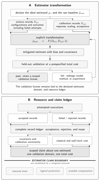
Error mitigation is an inference pipeline. Science and calibration records feed an explicit estimator, while bias, covariance, acceptance, validation, and total cost delimit a claim about one declared estimand. The boundary bars prevent an estimator improvement from being relabeled as state restoration or encoded protection.

Combine Methods Without Double Counting

Composition order changes the estimator

A stack is a new estimator, not a bag of independently certified modules. Measurement correction followed by symmetry conditioning need not equal conditioning followed by response correction. Noise scaling can change the calibration model; dynamical suppression can change acceptance; a projection can make a later extrapolation nonlinear. Write the ordered composition explicitly, including which records and parameters enter each step.

For transformations $F_1$ and $F_2$, the notation $F_2(F_1(D))$ should be treated as a hypothesis about target preservation and transfer. Check whether the output object of $F_1$ satisfies the input assumptions of $F_2$. If $F_1$ changes the estimand or acquisition distribution, a license proven for $F_2$ on raw records does not automatically survive.

Order also determines resource and failure accounting. A rejected record may still have consumed all upstream operations, and calibration needed before rejection is not saved by a low acceptance rate. Report where failures occur and which downstream costs they avoid.

Shared records create covariance and reuse constraints

Two mitigation components may use the same shots, calibration model, or training set. Shared records create statistical dependence, while shared calibration creates correlated systematic uncertainty. Adding component variances as if they were independent can overstate or understate the final uncertainty. Reusing a record is computationally efficient, but it does not create independent evidence.

Shared data can also blur tuning and validation roles. If one method’s residuals choose another method’s settings, the complete stack has been tuned on those records. A calibration reused across components needs a common expiry and transfer argument, or component-specific evidence showing why the domains differ. Track each record through a data-flow diagram or machine-readable provenance ledger.

Double counting appears in resource claims too. The same calibration cost should not be charged twice within one run, but neither should it vanish from both components. Assign it once to the stack and state the workload over which it is amortized. Report marginal component costs alongside the complete stack total.

Tune once and validate the full stack

Freeze method order, hyperparameters, calibration rules, stopping criteria, and software before the held-out comparison. Component-level demonstrations can motivate a stack, but they do not validate it. The full procedure may amplify a residual that each component tolerates separately, and model errors can align rather than cancel.

Use validation tasks that stress the joint assumptions: calibration transfer after suppression, acceptance across scaling points, covariance under record reuse, and estimator stability near the chosen regularization. Failed validation should return the workflow to model, method, or experiment redesign. Reusing the same held-out set after redesign converts it into tuning data; a new final test is then required.

Successful stack validation licenses only the frozen composition and domain. It does not show that each component was necessary. Ablations at matched resources can reveal whether a simpler procedure performs as well and can identify unnecessary variance or calibration burden.

Validate on Held-Out Tasks and Report the Result

Use independent truth or bounded references

The strongest validation compares against independently known ideal values: analytic solutions, exact classical calculations within a documented regime, or a trusted higher-quality experiment. Independence concerns data and modeling decisions. A reference derived from the same fitted noise model can check internal consistency but cannot independently test model mismatch.

When exact truth is unavailable, state the reference’s bound, uncertainty, and validity domain. Cross-platform agreement can be useful but does not prove correctness under shared assumptions. Conservation laws and limiting cases test selected features, not the full target. Several imperfect references can triangulate a claim if their dependencies are disclosed.

Choose validation tasks to represent the intended science domain, including hard cases and null effects. A benchmark family selected because mitigation performs well cannot support a population claim without accounting for that selection. Algorithmic Benchmarking owns end-to-end task and cost comparisons; this page supplies the estimator-level record that such a benchmark must carry.

Compare at fixed quality, confidence, and cost

Raw and mitigated procedures must estimate the same target over the same task distribution. Compare loss at equal total cost, or compare total cost needed to meet the same quality and confidence. A fixed science-shot comparison is insufficient when one procedure consumes extra calibration, rejects records, or runs longer circuits. Likewise, equal attempt count can conceal unequal wall time and drift exposure.

Report uncertainty on the performance comparison itself. Four favorable tasks can demonstrate those four outcomes, but they provide weak evidence for transfer to a broad population. Paired task designs can improve precision because raw and mitigated errors on the same task are correlated; the analysis should retain that pairing. Predeclare the aggregation and treatment of failures.

A finite cost-matched improvement is valuable when worded narrowly. It says that the frozen mitigated procedure improved the chosen loss on the prespecified held-out set at the declared resources. It does not establish universal advantage, asymptotic scaling, physical state recovery, or robustness to untested drift.

Report raw results, failures, and validity domains

Publish enough of the raw and transformed record to reproduce the estimator and diagnose reversals. This includes circuit and control versions, timestamps and acquisition order, calibration data or sufficient summaries, signed weights, covariance, rejected branches, failures, code versions, and exact task partitions. Report negative as well as positive held-out outcomes.

Reporting Standards owns the durable provenance and artifact infrastructure. The compact ledger below states what the mitigation claim contributes. Empty cells are evidence gaps, not permission to assume zero uncertainty or cost.

Ledger item	Raw record	Transformed record	Uncertainty	Cost
Estimand and baseline	Ideal target and best raw procedure	Claimed mitigated target	Reference bound	Baseline resources
Calibration or training	Samples, context, and epoch	Fitted parameters and expiry	Fit and transfer error	Acquisition and fitting
Science configurations	Counts at every setting	Included records	Shot and batch variation	All attempted executions
Weights or nonlinear transform	Component estimates	Formula and frozen tuning	Sensitivity or coverage	Extra settings and compute
Covariance	Paired and shared records	Complete matrix or model	Estimation uncertainty	Pairing and storage
Acceptance and failures	Accepted, rejected, invalid, timed out	Conditional target and rate	Ratio or sequential uncertainty	All attempts
Validation reference	Truth, bound, or proxy	Held-out residuals	Reference uncertainty	Reference executions
Total resources	Raw procedure total	Full stack total	Amortization range	Classical and wall-clock total

The validity domain belongs beside the headline result. Name circuits, devices, contexts, epochs, observable classes, acceptance regime, and resource range. A machine-readable record is desirable, but a clear human-readable statement remains necessary so downstream authors do not overextend the result.

Know When Mitigation Is the Wrong Intervention

Lost distinguishability creates sampling pressure

Noise can make different ideal outputs nearly indistinguishable. An estimator required to infer that distinction uniformly from those noisy output records, without an external computation that already supplies the answer, must then amplify small observed distinctions. This raises sensitivity to sampling and model error. Large inverse-response condition numbers, large signed-weight norms, or vanishing acceptance are finite diagnostics of this pressure.

General limitation results formalize such tradeoffs under specified protocol and resource models. Takagi et al. (2022) derive fundamental bounds for classes of mitigation, and Takagi, Tajima, and Gu (2023) establish universal sampling lower bounds in a defined framework. Quek et al. (2024) obtain tighter limitations in regimes covered by their assumptions. These results should inform resource forecasts and stop rules, not be detached from their hypotheses to declare every finite mitigation task impossible.

Before adding a more aggressive inverse, ask whether better controls, a more informative measurement, a narrower target, or a redesigned circuit preserves more distinguishability. An unstable statistical recovery is often a symptom that the experiment is not generating enough target-relevant information.

Deep scalable protection is an architectural question

Finite mitigation can extend the useful range of shallow or moderate experiments, support verification, and improve selected observables. Those are meaningful goals. They do not answer how errors accumulate through arbitrarily deep computation, how logical operations contain faults, or how resource overhead scales at a target logical error rate.

Those questions require encoded quantum error correction and fault-tolerant architecture. The error model, syndrome extraction, decoder, logical gates, leakage handling, and threshold assumptions all matter. A mitigation layer may coexist with them—for example, to improve a finite logical observable—but it cannot replace evidence for protection throughout the computation.

The converse overstatement is also wrong. The need for fault tolerance at scale does not make every pre-fault-tolerant estimator scientifically useless. Choose the intervention by the task horizon: control improvement for avoidable physical errors, mitigation for bounded output estimation when its license and cost work, and encoded protection when information must survive deep noisy operations.

Stop, redesign, or escalate when assumptions fail

Predeclare stop conditions. Examples include response residuals beyond tolerance, non-transfer across contexts, scaling that changes an ideal proxy, coefficient norms above the feasible precision budget, acceptance below a useful threshold, calibration drift before workload completion, undercoverage in validation, or cost exceeding the best raw alternative. A stop is an experimental result, not a missing success.

Redesign can act at several levels. Improve calibration or physical control; change acquisition order; choose a better-conditioned observable; reduce circuit depth; narrow the validity domain; or replace the estimator. Escalate to encoded correction when the task requires persistent quantum information rather than a finite output estimate. Do not keep adding transformations after held-out failure and continue calling the same records a test.

Negative Results and Limitations owns durable reporting of no-go scope, benchmark reversals, and failed transfers. The local conclusion is narrower: a proposed mitigation procedure is justified only while its estimand, uncertainty, validation, and total-resource ledgers remain intact.

Three Reproducible Estimator Audits

Audit 1 — A covariance-aware signed estimator

Take observed means $(0.71,0.64)$, weights $(2,-1)$, and covariance matrix

$$\Sigma= \begin{pmatrix} 0.0009&0.0003\\ 0.0003&0.0016 \end{pmatrix}.$$

The signed estimate is $0.78$. The complete quadratic form gives variance $0.004$ and standard deviation $\sqrt{0.004}$, whereas discarding the off-diagonal entries gives $0.0052$. The absolute-weight sum is $3$. Its square, $9$, is an overhead scale only for independent components with equal per-shot variance and optimal allocation proportional to absolute weight. It is not the variance of this correlated design and says nothing about whether a physical noise-scaling model is valid.

Audit 2 — A postselection target and acceptance ledger

Among $1000$ attempts, accepted outcomes contain $420$ plus and $180$ minus records; rejected outcomes contain $260$ plus and $140$ minus records. Thus $600$ attempts are accepted, $a=0.6$, the accepted conditional signed mean is $0.4$, and the unconditioned accepted signed contribution is $0.24$. The rejected-branch conditional signed mean is $0.3$, another reminder that rejection is not absence of data.

For stationary independent attempts at fixed $a$, an expected $5000$ accepted samples require $5000/0.6$ attempts and $5000/0.6-5000$ rejected attempts. The expectation is not a guarantee, and the formula is not transferred to drifting or adaptive acceptance without a process model.

Audit 3 — A held-out comparison at matched attempt count

On four prespecified held-out targets $(0.20,0.40,0.60,0.80)$, compare raw estimates $(0.16,0.35,0.55,0.71)$ with mitigated estimates $(0.19,0.42,0.58,0.79)$. The raw procedure uses $12000$ attempts. The mitigated procedure uses $10000$ science and $2000$ calibration attempts, so the attempted-execution counts match. Its root-mean-square error is smaller on this set at this declared attempt budget. This fixture does not establish equal wall-clock, control, or classical cost, and it licenses no claim about unseen tasks, restored states, or universal transfer.

const tolerance = 1e-12;
const close = (actual, expected) => {
  if (Math.abs(actual - expected) > tolerance) throw new Error(`${actual} != ${expected}`);
};
const requireTrue = (condition) => {
  if (!condition) throw new Error('audit assertion failed');
};

const means = [0.71, 0.64];
const weights = [2, -1];
const covariance = [[0.0009, 0.0003], [0.0003, 0.0016]];
const estimate = weights.reduce((sum, weight, row) => sum + weight * means[row], 0);
const fullVariance = weights.reduce(
  (sum, leftWeight, row) => sum + weights.reduce(
    (inner, rightWeight, column) => inner + leftWeight * covariance[row][column] * rightWeight,
    0,
  ),
  0,
);
const diagonalVariance = weights.reduce(
  (sum, weight, row) => sum + weight * weight * covariance[row][row],
  0,
);
const standardDeviation = Math.sqrt(fullVariance);
const absoluteWeightSum = weights.reduce((sum, weight) => sum + Math.abs(weight), 0);
const independentEqualVarianceOptimalAllocationScale = absoluteWeightSum ** 2;
close(estimate, 0.78);
close(fullVariance, 0.004);
close(diagonalVariance, 0.0052);
close(standardDeviation, Math.sqrt(0.004));
close(absoluteWeightSum, 3);
close(independentEqualVarianceOptimalAllocationScale, 9);

const acceptedCounts = { plus: 420, minus: 180 };
const rejectedCounts = { plus: 260, minus: 140 };
const targetAcceptedSamples = 5000;
const accepted = acceptedCounts.plus + acceptedCounts.minus;
const rejected = rejectedCounts.plus + rejectedCounts.minus;
const attempts = accepted + rejected;
const acceptance = accepted / attempts;
const conditionalSignedMean = (acceptedCounts.plus - acceptedCounts.minus) / accepted;
const unconditionalAcceptedContribution = (acceptedCounts.plus - acceptedCounts.minus) / attempts;
const rejectedConditionalSignedMean = (rejectedCounts.plus - rejectedCounts.minus) / rejected;
const expectedAttempts = targetAcceptedSamples / acceptance;
const expectedRejectedAttempts = expectedAttempts - targetAcceptedSamples;
close(attempts, 1000);
close(accepted, 600);
close(rejected, 400);
close(acceptance, 0.6);
close(conditionalSignedMean, 0.4);
close(unconditionalAcceptedContribution, 0.24);
close(rejectedConditionalSignedMean, 0.3);
close(expectedAttempts, 5000 / 0.6);
close(expectedRejectedAttempts, 5000 / 0.6 - 5000);

const idealHeldOut = [0.20, 0.40, 0.60, 0.80];
const rawEstimates = [0.16, 0.35, 0.55, 0.71];
const mitigatedEstimates = [0.19, 0.42, 0.58, 0.79];
const rmse = (estimates) => Math.sqrt(estimates.reduce(
  (sum, value, position) => sum + (value - idealHeldOut[position]) ** 2,
  0,
) / idealHeldOut.length);
const rawRmse = rmse(rawEstimates);
const mitigatedRmse = rmse(mitigatedEstimates);
const rawTotalAttempts = 12000;
const mitigatedScienceAttempts = 10000;
const mitigatedCalibrationAttempts = 2000;
const mitigatedTotalAttempts = mitigatedScienceAttempts + mitigatedCalibrationAttempts;
close(rawRmse, Math.sqrt(0.003675));
close(mitigatedRmse, Math.sqrt(0.00025));
close(rawTotalAttempts, mitigatedTotalAttempts);
requireTrue(mitigatedRmse < rawRmse);

console.log('Error-mitigation estimator audits: PASS');

Canonical Owners and Common Claim Failures

Canonical handoffs

The chapter guide Noise, Channels, and Error Mitigation owns the broader discrepancy-to-model record, and Noise in Quantum Information owns the device-facing mechanism taxonomy. Quantum Measurement as Estimation owns general decision theory. SPAM Errors owns preparation–measurement identifiability. Algorithmic Benchmarking owns end-to-end application comparisons, Reporting Standards owns durable artifacts, and Negative Results and Limitations owns durable no-go and failure scope.

Measurement Error Mitigation, Zero-Noise Extrapolation, Probabilistic Error Cancellation, Symmetry Verification, Dynamical Decoupling, and Limits of Error Mitigation remain specialist handoffs. Their algorithms and proofs should not be inferred from this cross-family workflow.

Common claim failures

A better number is called a corrected state. Report an improved estimate of the named quantity unless separate state-level evidence exists.

Bias is quoted without covariance or cost. Propagate the complete acquisition design and compare accepted-answer procedures at matched resources.

Postselection silently changes the target. Distinguish conditional expectation, unconditioned accepted contribution, and the original ideal estimand.

Exact-model unbiasedness is called robustness. Include calibration, mismatch, drift, selection, and regularization effects.

Validated components are treated as a validated stack. Freeze the ordered composition and test it end to end on held-out tasks.

One failure is called a universal impossibility—or one success a scalable architecture. Keep both limitation and success claims inside their protocol, domain, and resource assumptions.

Exercises

1. Classify seven interventions. Classify pulse retuning, dynamical decoupling, response-matrix inversion, noise extrapolation, signed cancellation, symmetry postselection, and syndrome-based logical recovery by what each changes. Give one required license for each.

Solution

Pulse retuning changes control and needs diagnostic transfer. Decoupling changes evolution and needs a spectral-control model. Response inversion, extrapolation, and cancellation transform estimates and respectively need a transferable response, target-preserving scaling, and an implementable learned basis. Postselection conditions records and needs a sector promise. Logical recovery protects encoded information and needs a correctable error set and fault model.

2. Propagate a signed estimator covariance. Recompute Audit 1 and explain the direction of the off-diagonal contribution. Under what restricted allocation assumptions does the factor $9$ apply?

Solution

$2(0.71)-0.64=0.78$. The covariance contribution is $2(2)(-1)(0.0003)=-0.0012$, so the full variance is $0.0036+0.0016-0.0012=0.004$. The diagonal result is $0.0052$. The factor $9=(|2|+|-1|)^2$ applies only to independent components with equal per-shot variance and optimal allocation proportional to absolute weight.

3. Include calibration uncertainty. A scalar calibration $\widehat\theta$ has variance $s_\theta^2$ and enters a smooth estimator $F(D,\theta)$. Give the leading calibration-variance term and name two reasons it may fail.

Solution

The leading term is $(\partial F/\partial\theta)^2s_\theta^2$, with cross terms when calibration and science records depend on one another. The approximation can fail near a singular inverse, a clipping boundary, or a small denominator. Strong nonlinearity, drift, and non-Gaussian finite samples can instead require hierarchical resampling or direct coverage simulation.

4. Distinguish conditional and unconditional targets. Use Audit 2 to calculate $\mathbb E[O\mid A]$ and $\mathbb E[O\mathbf1_A]$. Explain why neither automatically estimates an original unconditional ideal expectation.

Solution

Acceptance is $600/1000=0.6$. The conditional signed mean is $(420-180)/600=0.4$; the unconditioned accepted contribution is $(420-180)/1000=0.24$. Conditioning changes the sampled population, while multiplying by the acceptance probability assigns zero to rejection. A theorem about the rejection mechanism and target is needed to connect either quantity to the original expectation.

5. Build a total-cost ledger. A procedure uses $8000$ science attempts, $1500$ calibration attempts, $500$ validation attempts, and accepts $75\%$ of science attempts. Report accepted science samples and total attempted executions; list two costs still missing.

Solution

It accepts $0.75(8000)=6000$ science samples and uses $8000+1500+500=10000$ recorded attempts. The ledger still needs failed or timed-out attempts if excluded from those totals, along with control expansion, reset, classical fitting, storage, wall-clock duration, queueing, or recalibration. Calibration amortization also needs a workload and stability interval.

6. Audit a stacked mitigation. A team applies suppression, response correction, and symmetry rejection, validating each separately. Identify three missing checks before claiming the stack improves an estimator.

Solution

Write and test the exact order, because suppression may change the response model and rejection may make the estimator nonlinear. Propagate covariance from shared science and calibration records and state reuse constraints. Freeze all tuning, then validate the complete stack on held-out tasks at matched total cost. Separate component validation cannot establish these joint properties.

7. Scope a mitigation-versus-QEC claim. Correct both statements: “all mitigation is exponentially useless” and “successful mitigation replaces fault tolerance.”

Solution

Lower bounds apply under declared protocol, noise, target, and resource models; they can imply severe sampling pressure without making every finite task useless. A finite held-out improvement licenses that estimator, domain, and cost, not state restoration or scalable computation. Deep reliable computation requires encoded protection and fault-tolerant operations under an appropriate fault model.

References

• X. Bonet-Monroig, R. Sagastizabal, M. Singh, and T. E. O’Brien, “Low-Cost Error Mitigation by Symmetry Verification,” Physical Review A 98, 062339 (2018), doi:10.1103/PhysRevA.98.062339.
• S. Bravyi, S. Sheldon, A. Kandala, D. C. McKay, and J. M. Gambetta, “Mitigating Measurement Errors in Multiqubit Experiments,” Physical Review A 103, 042605 (2021), doi:10.1103/PhysRevA.103.042605.
• Z. Cai, R. Babbush, S. C. Benjamin, S. Endo, W. J. Huggins, Y. Li, J. R. McClean, and T. E. O’Brien, “Quantum Error Mitigation,” Reviews of Modern Physics 95, 045005 (2023), doi:10.1103/RevModPhys.95.045005.
• S. Endo, S. C. Benjamin, and Y. Li, “Practical Quantum Error Mitigation for Near-Future Applications,” Physical Review X 8, 031027 (2018), doi:10.1103/PhysRevX.8.031027.
• E. Knill and R. Laflamme, “Theory of Quantum Error-Correcting Codes,” Physical Review A 55, 900–911 (1997), doi:10.1103/PhysRevA.55.900.
• Y. Li and S. C. Benjamin, “Efficient Variational Quantum Simulator Incorporating Active Error Minimization,” Physical Review X 7, 021050 (2017), doi:10.1103/PhysRevX.7.021050.
• F. B. Maciejewski, Z. Zimborás, and M. Oszmaniec, “Mitigation of Readout Noise in Near-Term Quantum Devices by Classical Post-Processing Based on Detector Tomography,” Quantum 4, 257 (2020), doi:10.22331/q-2020-04-24-257.
• Y. Quek, D. Stilck França, S. Khatri, J. J. Meyer, and J. Eisert, “Exponentially Tighter Bounds on Limitations of Quantum Error Mitigation,” Nature Physics 20, 1648–1658 (2024), doi:10.1038/s41567-024-02536-7.
• R. Takagi, S. Endo, S. Minagawa, and M. Gu, “Fundamental Limits of Quantum Error Mitigation,” npj Quantum Information 8, 114 (2022), doi:10.1038/s41534-022-00618-z.
• R. Takagi, H. Tajima, and M. Gu, “Universal Sampling Lower Bounds for Quantum Error Mitigation,” Physical Review Letters 131, 210602 (2023), doi:10.1103/PhysRevLett.131.210602.
• K. Temme, S. Bravyi, and J. M. Gambetta, “Error Mitigation for Short-Depth Quantum Circuits,” Physical Review Letters 119, 180509 (2017), doi:10.1103/PhysRevLett.119.180509.
• L. Viola and S. Lloyd, “Dynamical Suppression of Decoherence in Two-State Quantum Systems,” Physical Review A 58, 2733–2744 (1998), doi:10.1103/PhysRevA.58.2733.