Device Characterization

Short Definition

Device characterization is the design and analysis of experiments that identify a predictive model of a quantum device, estimate its parameters and uncertainties, and test where that model fails. It asks not merely how large an error is, but what mechanism, context, and timescale explain the observed behavior.

For an experimental setting $x$, outcome $y$, and model parameters $\boldsymbol\theta$, a common starting point is

$$p_{\boldsymbol\theta}(y|x) = \operatorname{Tr} \!\left[ M_{y|x}\, \mathcal E_{\boldsymbol\theta,x}(\rho_x) \right].$$

Characterization turns the observed counts into claims about $\boldsymbol\theta$, but only after declaring the prepared states $\rho_x$, measurement effects $M_{y|x}$, channel family $\mathcal E_{\boldsymbol\theta,x}$, and system boundary. The result may be a transition frequency, a relaxation rate, a Hamiltonian, a gate set, a correlated-noise model, or evidence that no member of the proposed family is adequate.

A fitted parameter table is therefore not enough. Mature characterization also establishes:

1. identifiability: the data distinguish the reported parameter combinations;
2. uncertainty: finite sampling and calibration uncertainty are propagated;
3. predictive validity: the model predicts held-out experiments;
4. scope: time window, circuit context, controls, neighbors, and leakage conventions are explicit;
5. actionability: the evidence supports a stated calibration, compilation, simulation, or monitoring decision.

Canonical Scope

This page owns the inverse problem of learning and validating device models:

• coherent versus incoherent error diagnosis;
• spectroscopy, time-domain amplification, and noise spectroscopy as a characterization workflow;
• Hamiltonian, generator, and gate-set identification;
• identifiability, gauge freedom, experiment design, residual checks, and model selection;
• SPAM, leakage, crosstalk, drift, non-Markovianity, and context dependence;
• the evidence record needed before a characterization result enters a calibration or software pipeline.

Noise in Quantum Information owns the physical and mathematical noise taxonomy. Process Tomography owns reconstruction of a channel under trusted preparation and measurement. Randomized Benchmarking and Cycle Benchmarking own their protocol derivations and reported metrics.

Control, Readout, and Calibration owns the physical control stack. Calibration Loops owns triggers, dependencies, validation gates, publication, and rollback. Here those ingredients are used for a distinct question: which predictive model is supported by the device records, and what evidence justifies acting on it?

Leakage and Crosstalk owns the QI-facing full-space, survival, leakage/seepage/coherence, flag, scalar-dynamics, and operational-locality model contract; this page retains experimental design, identifiability, gauge-aware estimation, model selection, residual checks, uncertainty, and the evidence needed before calibration or software action.

Characterization Is Not a Synonym for Benchmarking

The same experiment can contribute to several workflows, but the inferential targets differ.

activity	primary question	typical output
characterization	what model explains and predicts the behavior?	frequencies, rates, generators, gate sets, correlations, residuals
benchmarking	how well does the device perform under a declared ensemble or task?	decay parameter, fidelity-like metric, success probability
calibration	which control setting should be changed?	a candidate parameter update plus validation evidence
verification	does the device or output satisfy a stated requirement?	pass/fail decision, bound, or rejected null

A randomized-benchmarking decay can reveal that performance changed without identifying whether the cause was detuning, dephasing, leakage, crosstalk, or readout drift. Conversely, a detailed Hamiltonian estimate need not summarize application performance. Treating one output as a substitute for the other creates false diagnoses.

Characterization is also different from explanation in the causal sense. An effective dephasing parameter can predict records while remaining agnostic about whether the microscopic source was flux noise, photon shot noise, temperature drift, or electronics. Causal attribution requires interventions or additional measurements that distinguish those hypotheses.

The Statistical Inverse Problem

Suppose setting $x$ is repeated $N_x$ times and produces counts $n_{y|x}$. Under a stationary independent-shot model,

$$\mathbf n_x \sim \operatorname{Multinomial} \!\left( N_x,\mathbf p_{\boldsymbol\theta,x} \right), \qquad N_x=\sum_y n_{y|x}.$$

Ignoring count-dependent constants, the log likelihood is

$$\ell(\boldsymbol\theta) = \sum_{x,y} n_{y|x} \log p_{\boldsymbol\theta}(y|x).$$

An estimator may maximize this likelihood, sample a posterior, or minimize a loss chosen for the noise model. The choice should follow the data-generating process. Least squares with constant variance is generally not equivalent to the binomial or multinomial likelihood near probabilities zero and one.

The parameter vector is meaningful only relative to a model family. For example, a driven qubit might be modeled by

$$\frac{d\rho}{dt} = -i \left[ H(\boldsymbol\theta,t),\rho \right] + \sum_\mu \gamma_\mu \mathcal D[L_\mu](\rho),$$

with

$$\mathcal D[L](\rho) = L\rho L^\dagger - \frac12 \left\{ L^\dagger L,\rho \right\}.$$

This equation does not become true because it fits one Rabi trace. The Markovian generator, operator basis, control transfer function, and time-independence assumptions all need tests.

Declare the estimand

A frequency estimated during a Ramsey experiment may be:

• a bare transition frequency;
• a dressed frequency under a continuous coupling;
• a detuning relative to a local oscillator;
• a time average over drift;
• a conditional frequency given neighboring-qubit states.

These are different estimands. Likewise, a gate can mean a pulse segment, a logical frame update, a calibrated schedule including buffers, or an effective operation after tracing out leakage levels. A useful characterization record defines the object before reporting its parameters.

Separate randomness from misspecification

Sampling uncertainty shrinks with more repetitions under a correct stationary model. Model discrepancy does not. If residual structure persists as shot count increases, shrinking confidence intervals around the wrong model only makes the report more precise, not more accurate.

Let $\widehat p_{y|x}=n_{y|x}/N_x$. A standardized residual is approximately

$$r_{y|x} = \frac{ \widehat p_{y|x} - p_{\widehat{\boldsymbol\theta}}(y|x) }{ \sqrt{ p_{\widehat{\boldsymbol\theta}}(y|x) \left[ 1-p_{\widehat{\boldsymbol\theta}}(y|x) \right] /N_x } },$$

for a binary outcome considered marginally. Runs, time order, experimental setting, circuit depth, and spectator configuration should be visible in residual plots. A single goodness-of-fit number can hide precisely the structure needed for diagnosis.

Identifiability and Observability

Parameters are globally identifiable when no distinct allowed parameter point produces the same distribution for every permitted experiment. They are locally identifiable near $\boldsymbol\theta_0$ when sufficiently small parameter changes alter the observable probabilities, apart from declared gauge freedoms.

For probabilities collected into a vector $\mathbf p$, define the sensitivity matrix

$$J_{ia} = \left. \frac{ \partial p_i }{ \partial\theta_a } \right|_{\boldsymbol\theta_0}.$$

Full column rank suggests local identifiability for an ordinary parameterization. A rank deficiency means that at least one infinitesimal parameter combination is invisible to the chosen experiments. In gate-set tomography, known gauge directions must first be quotiented out; demanding rank along those directions is a category error.

For multinomial experiments, the classical Fisher information is

$$\mathcal I_{ab}(\boldsymbol\theta) = \sum_x N_x \sum_y \frac{ \partial_a p_{\boldsymbol\theta}(y|x) \, \partial_b p_{\boldsymbol\theta}(y|x) }{ p_{\boldsymbol\theta}(y|x) }.$$

When regularity conditions hold, an unbiased estimator obeys

$$\operatorname{Cov} \!\left( \widehat{\boldsymbol\theta} \right) \succeq \mathcal I(\boldsymbol\theta)^{-1}.$$

The eigenvectors of $\mathcal I$ reveal well- and poorly-constrained combinations. A large condition number warns that nominally identifiable parameters may be practically inseparable at the available shot budget. Profile likelihoods or posterior marginals are often more informative than one standard error per coordinate when the likelihood is curved, bounded, or multimodal.

Identifiability is designed, not merely checked

Repeating an insensitive experiment does not recover a missing parameter. Useful experimental design varies:

• preparation and measurement axes;
• evolution time and pulse phase;
• sequence length and ordering;
• spectator states and simultaneous operations;
• delay between experiments;
• control amplitude and detuning;
• filter functions for distinct frequency bands.

For a candidate design $\xi$, common criteria include maximizing $\log\det\mathcal I(\xi)$ for joint precision, maximizing the smallest eigenvalue for worst-direction precision, or maximizing expected information gain

$$\mathbb E_{y|\xi} \left[ D_{\mathrm{KL}} \!\left( p(\boldsymbol\theta|y,\xi) \Vert p(\boldsymbol\theta) \right) \right].$$

Adaptive design can use current uncertainty to choose the next setting. Its selection rule, stopping condition, and complete trial history must be recorded, because adaptivity changes the sampling design and can invalidate naive uncertainty calculations.

Choose a Model Hierarchy

Characterization should begin with the least complex family that can answer the operational question, then expand only when predictive checks demand it. A useful hierarchy is:

1. a constant scalar parameter, such as one detuning or readout contrast;
2. a time-independent Hamiltonian model;
3. a Markovian completely positive generator;
4. a gate-dependent channel or self-consistent gate set;
5. a context-dependent model conditioned on spectators or schedules;
6. a time-varying or hidden-state model for drift and memory;
7. an explicitly non-Markovian process model.

Complexity must be paid for with informative data. A model can interpolate a calibration suite while being nonidentifiable and useless for prediction. Conversely, a visibly inadequate simple model should not be retained merely because its parameters have small formal error bars.

The system boundary matters throughout. Tracing out a resonator, spectator, leakage level, or fluctuating classical variable can turn simple joint dynamics into non-Markovian reduced dynamics. “Non-Markovian noise” may therefore diagnose a boundary choice rather than a unique microscopic mechanism.

Coherent and Incoherent Errors

A useful first distinction is whether errors preserve purity while rotating the state incorrectly, or irreversibly contract distinguishability in the modeled subsystem.

Coherent miscalibration

For a target qubit rotation

$$G = \exp \!\left( -i\frac{\theta}{2} \widehat{\mathbf n}\cdot\boldsymbol\sigma \right),$$

an overrotation by $\epsilon$ gives

$$\widetilde G = \exp \!\left( -i\frac{\theta+\epsilon}{2} \widehat{\mathbf n}\cdot\boldsymbol\sigma \right).$$

When the error commutes with the target, $m$ repetitions accumulate angle $m\epsilon$. Yet the single-gate average infidelity of the unitary error is

$$r = \frac23 \sin^2 \!\left( \frac{\epsilon}{2} \right) \approx \frac{\epsilon^2}{6}.$$

This contrast explains why error-amplifying sequences are powerful: a quadratic one-gate metric can conceal a phase displacement that grows linearly with sequence length. Alternating target and inverse gates, repeating a nominal identity-generating block, or selecting matrix elements that carry the coherent phase can isolate the signed error.

Coherent does not mean stable. A detuning that is approximately constant during each circuit but varies between circuits produces coherent evolution within a shot and ensemble dephasing across shots. The correct model depends on the timescale at which the parameter fluctuates.

Incoherent contraction

Amplitude damping, Markovian dephasing, stochastic Pauli errors, and coupling to unresolved degrees of freedom contract at least some Bloch-vector directions. A unital qubit map can be written

$$\mathbf r' = T\mathbf r+\mathbf t,$$

where $T$ describes contraction and rotation and $\mathbf t$ describes nonunital translation. Unitary error has orthogonal $T$ and preserves $|\mathbf r|$; incoherent error generally reduces purity for at least some inputs.

The distinction is model relative. Leakage is coherent in a larger Hilbert space but appears nonunitary after projection onto the computational subspace. Low-frequency classical noise can look like a deterministic rotation over a short record and like dephasing over a long one.

No single scalar cleanly partitions all realistic noise. Useful evidence combines phase-sensitive amplification, purity-sensitive experiments, sequence-length dependence, and context variation.

Spectroscopy and Time-Domain Diagnostics

Component-level experiments identify interpretable parameters before larger gate-set models are attempted.

Transition spectroscopy

A weak probe scanned in frequency locates resonances and line shapes. Splittings can reveal coupling, avoided crossings, spectator-state conditioning, or multilevel structure. The measured peak need not equal the undriven transition frequency: power broadening, ac Stark shifts, line pulling, and finite pulse duration can move or reshape it.

Peak fitting should compare plausible line-shape models and include frequency reference uncertainty. A residual that changes sign across a resonance often contains more diagnostic information than the fitted center alone.

Rabi experiments

Under a rotating-wave model, a driven two-level system with detuning $\Delta$ and on-resonance Rabi rate $\Omega$ oscillates at

$$\Omega_R = \sqrt{ \Omega^2+\Delta^2 }.$$

Amplitude sweeps calibrate rotation rate; time-frequency “chevrons” separate detuning from drive strength and expose additional transitions. Decay of the oscillation envelope is not automatically $T_2$: drive-amplitude noise, rotating-frame relaxation, leakage, and readout contrast can all contribute. The canonical Rabi and Ramsey Control page develops the driven dynamics.

Relaxation and dephasing

An idealized energy-relaxation experiment prepares the excited state, waits, and measures

$$P_1(t) = P_\infty + A e^{-t/T_1}.$$

A Ramsey experiment estimates detuning and inhomogeneous coherence time:

$$P_1(t) = B + A\,C(t) \cos \!\left( \Delta t+\phi \right).$$

The envelope $C(t)$ may be exponential, Gaussian, stretched exponential, or nonmonotonic. Choosing one form by habit can bias both frequency and coherence estimates. Under a narrow Markovian two-level model,

$$\frac1{T_2} = \frac1{2T_1} + \frac1{T_\phi},$$

but this relation is not a universal identity. Ramsey $T_2^*$, echo $T_2$, driven $T_{1\rho}$, and dynamical-decoupling coherence probe different spectral and timescale windows.

Interleaving reference measurements and preserving acquisition order help distinguish genuine envelope shape from drift. Error bars based only on binomial shot noise are inadequate when the frequency changes across the scan.

Noise Spectroscopy

Controlled modulation converts temporal noise into measurable decay. For classical Gaussian dephasing noise $\beta(t)$ and a modulation function $y(t)$, one common convention gives

$$C(T) = \exp \!\left[ -\chi(T) \right],$$

with

$$\chi(T) = \frac1{2\pi} \int_{-\infty}^{\infty} S_\beta(\omega) \left| Y(\omega,T) \right|^2 d\omega,$$

and

$$Y(\omega,T) = \int_0^T y(t)e^{i\omega t}\,dt.$$

Pulse sequences change the filter $|Y(\omega,T)|^2$. Measurements with several filters support an inverse estimate of the spectrum $S_\beta(\omega)$. The inverse problem is usually ill-conditioned: finite sequence duration limits frequency resolution, control imperfections alter the filter, and distinct spectra can produce nearly identical decays.

A trustworthy spectrum therefore states the basis or regularization used for reconstruction, the accessible frequency band, control-pulse model, and uncertainty or resolution kernel. Noise Spectra owns the spectral-density definitions; Dynamical Decoupling owns the control method.

Noise spectroscopy can suggest mechanisms, but spectral shape alone rarely identifies a unique physical source. Temperature, bias, drive power, and coupling interventions are often needed to test attribution.

Error-Amplifying Sequences

Small signed errors are easier to estimate when an experiment maps them to a large observable displacement. If a sequence family produces

$$p_m = A + B\cos \!\left( m\epsilon+\phi \right),$$

then multiple lengths $m$ identify $\epsilon$ much more precisely than a single near-identity experiment, provided decoherence and phase wrapping are modeled.

Useful constructions include:

• repeated overrotations for amplitude error;
• alternating axes for quadrature and phase error;
• repeated identity-generating gate blocks;
• echo-like cancellation of known terms;
• matrix-element amplification that selects one generator component.

Amplification can also magnify model failure. A fit that assumes one constant $\epsilon$ may fail under heating, pulse distortion, or gate-history dependence. Residuals versus length and sequence structure are therefore part of the result, not a cosmetic fit diagnostic.

Iterative randomized benchmarking is one such diagnostic strategy, but its interpretation depends on the randomization and error model. It should not be treated as a universal decomposition of coherent and incoherent error.

Process Tomography as a Diagnostic

Trusted-input process tomography estimates an effective channel and can expose axis tilt, nonunitality, contraction, and leakage-aware trace loss. In a Pauli transfer representation,

$$\begin{pmatrix} 1\\ \mathbf r' \end{pmatrix} = \begin{pmatrix} 1 & \mathbf 0^{\mathsf T}\\ \mathbf t & T \end{pmatrix} \begin{pmatrix} 1\\ \mathbf r \end{pmatrix}.$$

The antisymmetric component of $T$ near the identity is sensitive to small Hamiltonian rotations, its singular values describe contraction, and $\mathbf t$ captures nonunital effects. These interpretations become coordinate dependent away from a stated target and basis.

Ordinary process tomography assigns discrepancies in nominal input preparations or output effects to the reconstructed process. It is therefore not self-consistent under unknown SPAM. The canonical Process Tomography page develops Choi-space reconstruction, physical estimators, and validation.

Gate-Set Tomography

Gate-set tomography (GST) estimates state preparation, measurement, and a set of gates self-consistently. In Liouville notation, a gate set is

$$\mathcal G = \left\{ |\rho\rangle\!\rangle, \langle\!\langle E|, G_1,\ldots,G_K \right\}.$$

For a sequence $s=(s_1,\ldots,s_L)$, the modeled probability is

$$p(s) = \langle\!\langle E| G_{s_L} \cdots G_{s_1} |\rho\rangle\!\rangle.$$

Because preparation and measurement are estimated with the gates, GST avoids the specific SPAM attribution error of ordinary process tomography. It does not make SPAM irrelevant or eliminate all assumptions. The model still assumes a Hilbert-space dimension, a sequence-independent gate set, a chosen Markovian structure, and sufficient control to construct informative circuits.

Fiducials, germs, and sequence lengths

Short fiducial sequences synthesize effective preparations and measurements that span the modeled state and effect spaces. Repeated germs amplify distinct gate-set error directions. Long-sequence GST uses circuits built from fiducials around repeated germs at increasing lengths. The design should amplify every non-gauge parameter direction; otherwise some errors remain unobservable even with many shots.

Long sequences improve sensitivity but also expose drift, leakage, and non-Markovianity. Those are not nuisances to suppress silently. A likelihood failure at long length can be evidence that the fixed Markovian gate-set model is inadequate.

Gauge freedom

For any invertible representation change $B$,

$$|\rho\rangle\!\rangle \longrightarrow B|\rho\rangle\!\rangle,$$ $$\langle\!\langle E| \longrightarrow \langle\!\langle E|B^{-1},$$

and

$$G_k \longrightarrow BG_kB^{-1}.$$

Every sequence probability is unchanged. Thus the individual matrix entries of $\rho$, $E$, and $G_k$ are not all experimentally identifiable. This is a coordinate freedom of the gate-set representation, not an ordinary statistical uncertainty that more data remove.

Gauge optimization chooses a representative, often near a target gate set, to make reports interpretable. Gauge-dependent quantities must not be presented as direct observables. Sequence probabilities and properly constructed operational predictions are gauge invariant; many decomposed error-generator coordinates are not.

Model testing is part of GST

A maximum-likelihood GST estimate should be compared with the saturated model and with simpler or richer alternatives. Large structured residuals can indicate:

• gate dependence on preceding or simultaneous operations;
• drift during data acquisition;
• leakage outside the modeled dimension;
• pulse-history dependence;
• nonstationary SPAM;
• insufficient germ or fiducial design.

Goodness-of-fit failure does not mean GST “failed.” It means the proposed gate set is not an adequate compression of the observations at their statistical precision. Reporting a high-precision gate matrix while omitting that failure reverses the purpose of characterization.

Randomized Diagnostics Are Complementary

Randomized protocols compress behavior over an ensemble of circuits and are often more robust to SPAM than direct tomography. They are valuable characterization inputs, but their decay parameters do not generally identify a unique mechanism.

Randomized benchmarking

Under the standard gate-independent Markovian model, reference randomized benchmarking fits a survival curve

$$P(m) = A p^m+B.$$

The nuisance constants absorb leading SPAM dependence, while $p$ summarizes average contraction over the randomized ensemble. Gate-dependent noise, leakage, nonstationarity, and temporal correlations can change the decay or its interpretation. A good exponential fit is evidence for a useful compression over the measured range, not proof that the microscopic noise is depolarizing.

Randomized Benchmarking owns the protocol and conversion between $p$ and average error. In a characterization campaign, RB is best used as:

• a stable sentinel for changes in average performance;
• a comparison before and after a candidate calibration;
• an experiment repeated across times, contexts, or simultaneous operations;
• one coordinate in a larger diagnostic record.

Interleaved RB can associate additional decay with a selected gate under specific assumptions, but it still does not uniquely decompose that gate’s Hamiltonian, stochastic, leakage, and context-dependent errors.

Unitarity

The unitarity of a trace-preserving channel quantifies how much the channel preserves the length of traceless operators on average. In an orthonormal operator basis, let $T$ be the block mapping traceless inputs to traceless outputs. Then

$$u(\mathcal E) = \frac1{d^2-1} \operatorname{Tr} \!\left( T^\dagger T \right).$$

A unitary channel has $u=1$, while a depolarizing channel with contraction $p$ has $u=p^2$. Unitarity benchmarking estimates this purity-like decay with reduced SPAM sensitivity and helps determine whether an observed infidelity could be dominated by coherent error.

Unitarity is not a literal fraction of coherent errors. Nonunital processes, leakage, gate dependence, and context can complicate the decomposition. Combining average infidelity with unitarity constrains the noise family more than either scalar alone, but it does not identify a generator.

Cycle benchmarking

Cycle benchmarking characterizes a repeated scheduled layer under Pauli randomization and can resolve Pauli-error information for that layer. This is particularly useful when the implemented object is a simultaneous gate cycle rather than an isolated primitive. The canonical Cycle Benchmarking page owns the protocol and fidelity statements.

Agreement among GST, RB, unitarity, and cycle benchmarking is not guaranteed, because they weight errors, contexts, and circuit depths differently. A disagreement is a diagnostic clue. It can point to gate dependence, coherent accumulation, SPAM, leakage, compilation context, or model failure.

Preparation and Readout Characterization

SPAM is operational behavior, not merely a nuisance constant. For a computational-basis readout, an assignment matrix

$$A_{y|z} = \Pr \!\left( \text{reported }y \mid \text{prepared }z \right)$$

summarizes classical confusion only under a trusted preparation model. Its off-diagonal entries reveal assignment asymmetry, while its condition number warns whether inversion will amplify sampling noise.

SPAM Errors owns the QI-facing preparation-map, POVM and instrument, assignment-license, nonidentifiability, gauge, context-transfer, and mitigation-boundary contract. Measurement Error Mitigation owns finite-record response correction once the model is licensed, including stable inverse or forward likelihood, constraints, calibration covariance, scalable structure, overhead, and held-out residual validation; this page retains experimental design, GST protocols, model selection, residual tests, uncertainty, held-out prediction, and calibration handoff.

This matrix does not characterize all measurement errors. State disturbance, measurement-induced transitions, correlated outcomes, leakage misclassification, and dependence on preceding controls require richer instruments or detector models. Measurement Tomography owns reconstruction of measurement effects and instruments.

Readout characterization should vary:

• computational state and leakage state;
• integration window and discrimination threshold;
• neighboring-qubit state;
• simultaneous readout pattern;
• delay from the preceding gate;
• reset and heralding history.

Preparation and measurement errors are often confounded. Self-consistent methods, independent physical references, or targeted interventions are needed to separate them. Calling every observed assignment error “readout error” silently assumes preparation is perfect.

Crosstalk and Context Dependence

A local gate description is inadequate when behavior depends on operations outside its nominal support. Let $c$ label a context such as spectator state, simultaneous gate pattern, compiler schedule, or previous pulse. The relevant model is then

$$\mathcal E_{g,c},$$

not one context-free channel $\mathcal E_g$.

Useful designs compare matched contexts:

$$\Delta q = q(g,c_1)-q(g,c_0),$$

where $q$ may be a frequency, error generator component, RB decay, leakage rate, or readout probability. Randomizing or interleaving contexts protects the comparison against slow drift.

Simultaneous experiments

Simultaneous RB compares a qubit’s decay with neighbors idle versus active. Simultaneous GST estimates conditional gate-set changes. Both can detect addressability loss, but neither alone identifies the physical path. Frequency collisions, residual couplings, shared controls, classical electronics, and readout interactions may produce similar signatures.

Factorial designs can vary several spectators and estimate interaction terms. For binary activity variables $c_j$, an effective response model might be

$$q(\mathbf c) = \beta_0 + \sum_j \beta_j c_j + \sum_{j<k} \beta_{jk}c_jc_k +\cdots.$$

Sparse assumptions can reduce the experiment count, but they must be tested. Pairwise scans cannot exclude higher-order correlated effects.

Context is part of the characterized object

An isolated two-qubit gate, the same pulse played during neighboring gates, and a compiler-scheduled layer are distinct physical processes. The result must identify which was measured. Extrapolating isolated-gate characterization to application circuits is an empirical hypothesis, not a definition.

Leakage and Loss

Let $P_{\mathrm{comp}}$ project onto the computational subspace. For input $\rho$ in that subspace, one leakage probability is

$$L(\rho) = 1 - \operatorname{Tr} \!\left[ P_{\mathrm{comp}} \mathcal E(\rho) \right].$$

Leakage differs from an ordinary computational error because leaked population can persist, alter later controls, and return through seepage. A single end-of-circuit leakage estimate does not determine these dynamics. Sequence-length experiments and explicit preparation of leakage levels can estimate both outward and return rates.

Postselecting leaked or lost trials changes the estimand. The conditional map on retained trials may look high fidelity even when the unconditional operation has unacceptable loss. Reports should provide retention probability, state dependence, and whether leakage events are detected in real time.

Projection onto the computational subspace can also turn coherent multilevel dynamics into an apparently stochastic trace-decreasing channel. Characterizing the larger space is often necessary to choose a corrective pulse.

Drift, Memory, and Non-Markovianity

A stationary estimate averages over whatever changed during acquisition. If $\boldsymbol\theta(t)$ drifts, the observed distribution is closer to

$$p(y|x) = \int p_{\boldsymbol\theta}(y|x) \, d\mu_x(\boldsymbol\theta),$$

where the mixing measure $\mu_x$ can depend on when setting $x$ was sampled. Sequentially scanning all times for one setting and then the next can confound time with setting.

Defenses include:

• randomized or interleaved acquisition order;
• timestamped shot blocks and environmental telemetry;
• repeated reference circuits;
• hierarchical or state-space models for $\boldsymbol\theta(t)$;
• change-point analysis;
• block bootstrap or other uncertainty methods that preserve correlations.

A simple state-space model is

$$\boldsymbol\theta_{k+1} = \boldsymbol\theta_k+\mathbf w_k,$$ $$y_k \sim p_{\boldsymbol\theta_k} \!\left( y_k|x_k \right),$$

where $\mathbf w_k$ describes parameter evolution. This can support online tracking, but process-noise assumptions must be validated rather than tuned only for smooth plots.

Tests for memory

Possible signatures of memory or non-Markovianity include:

• sequence probabilities depending on earlier sequence history;
• residual autocorrelation after conditioning on the fitted model;
• incompatible estimates from experiments at different lengths;
• reduced-dynamics maps that fail a divisibility model;
• predictive improvement when hidden state or history is included.

No one signature identifies a unique quantum memory mechanism. Classical drift, heating, pulse distortion, and unmodeled spectators can produce similar records. “Non-Markovian” should describe the tested model failure and system boundary, not serve as a catch-all explanation.

Markovian and Non-Markovian Noise owns the QI-facing composition claim ladder, causal-break witness, alternative-explanation matrix, and scoped memory conclusion; this page retains experimental design, model selection, residual tests, uncertainty, held-out prediction, and calibration handoff.

Model Validation and Selection

Parameter estimation asks which point in a model family fits best. Model validation asks whether that family predicts the experiment well enough for the intended decision.

Held-out prediction

Reserve circuits, times, contexts, or sequence lengths that are not used for fitting. For held-out records $D_{\mathrm{test}}$, evaluate a proper predictive score such as

$$\ell_{\mathrm{test}} = \sum_{(x,y)\in D_{\mathrm{test}}} n_{y|x} \log p_{\widehat{\boldsymbol\theta}}(y|x).$$

Holding out random shots from every identical circuit tests sampling prediction but not extrapolation. Holding out entire sequence families, contexts, or later time blocks is a stronger test of the relevant generalization.

Compare nested and nonnested models

Likelihood-ratio tests can compare regular nested families when their asymptotic conditions apply. Information criteria or cross-validation can compare predictive tradeoffs, but singular models, boundary parameters, gauge freedom, and adaptive designs can invalidate textbook asymptotics. Parametric bootstrap or posterior predictive checks are often safer for complex gate models.

A more complex model is justified when it resolves structured residuals and improves out-of-sample prediction enough to matter operationally. Additional parameters that merely absorb shot noise do not constitute physical insight.

Propagate uncertainty into decisions

Characterization uncertainty should flow to the downstream quantity. If a calibration update is $u=f(\boldsymbol\theta)$, then near the estimate

$$\operatorname{Cov}(\widehat u) \approx J_f \operatorname{Cov} \!\left( \widehat{\boldsymbol\theta} \right) J_f^{\mathsf T}.$$

For nonlinear, constrained, or multimodal problems, samples from a bootstrap or posterior are preferable to this linear approximation. Systematic uncertainty in reference frequencies, pulse transfer functions, and trusted SPAM models should be propagated separately from shot noise.

From Diagnosis to Calibration

Characterization supports a calibration change only after the model has survived an action-relevant prediction. The workflow is iterative.

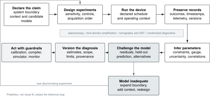
A characterization cycle begins with a declared claim, system boundary, and candidate model. Experiments identify parameters and uncertainty; residuals and held-out predictions decide whether to publish a versioned diagnostic record or expand the model and redesign the experiment.

A defensible handoff includes:

1. the diagnosed parameter and uncertainty;
2. evidence that the parameter is identifiable in the chosen design;
3. residual and held-out checks;
4. the proposed control change and its predicted effect;
5. independent validation metrics;
6. a rollback condition and the configuration versions involved.

The calibration loop should not fit and certify on the same record. After an update, acquire fresh validation data that include both the targeted diagnostic and a broader metric capable of detecting collateral damage. A detuning correction may improve a Ramsey fit while worsening leakage or neighboring-qubit crosstalk.

The canonical Calibration Loops page develops scheduling, dependency graphs, publication, and rollback.

A Minimum Characterization Record

field	what to report
object	qubits, couplers, modes, gates, pulse schedule, and system boundary
context	spectators, simultaneous operations, compiler and firmware versions
acquisition	timestamps, order randomization, shots, repetitions, exclusions
model	states, effects, dynamics, dimension, stationarity, and Markov assumptions
design	settings, sequence families, lengths, adaptivity, stopping rule
estimator	likelihood or loss, constraints, priors, optimization details
identifiability	rank or information analysis, gauge treatment, weak directions
uncertainty	intervals or regions, correlation structure, systematic budget
validation	residuals, held-out records, alternative models, goodness of fit
result	parameter estimates, operational invariants, and limits of interpretation
action	downstream calibration or model update, validation gate, rollback
provenance	raw-data identifier, code version, random seeds, configuration hashes

Machine-readable records should retain the count data or sufficient statistics, not only fitted curves and rounded parameter tables. Timestamps and acquisition order are essential for later drift audits.

Common Mistakes

Calling a fit a characterization

A smooth curve and small covariance matrix do not establish identifiability or model adequacy. Show residuals and predictive checks.

Treating a benchmark scalar as a mechanism

An RB decay, process fidelity, or quantum volume result can detect change without diagnosing its cause. Use mechanism-sensitive experiments.

Assuming coherent means unitary forever

Slowly varying detuning is coherent within one circuit and dephasing across an ensemble. State the averaging timescale.

Inverting a readout matrix without stability analysis

An ill-conditioned assignment matrix amplifies noise and model error. Mitigation needs uncertainty propagation and validation on independent states.

Ignoring gauge freedom in GST

Gauge-optimized matrix entries are representation dependent. Report operational predictions and identify gauge-dependent decompositions.

Scanning settings in a drift-confounded order

Acquiring each setting in one contiguous block can turn temporal drift into a false setting dependence. Randomize or interleave the design.

Discarding leakage

Postselection can hide the dominant failure mode. Report unconditional loss and the fate of leaked population.

Expanding the model without expanding the evidence

More parameters can reduce in-sample residuals while destroying identifiability. New model directions require new experimental sensitivity.

Updating calibration from the fitting data alone

Optimization and validation on one data set bias the apparent improvement. Use fresh validation records and broader guardrail metrics.

Research Status

Several foundations are mature: Rabi and Ramsey diagnostics, relaxation measurements, likelihood-based tomography, randomized benchmarking under declared models, GST gauge structure, and filter-function noise spectroscopy. Their limitations are also well understood.

Active work concerns scalable characterization of many-qubit context dependence, efficient learning of sparse correlated noise, robust online Hamiltonian learning, non-Markovian and drift-aware models, leakage-aware logical characterization, and experiment design that targets application predictions rather than complete process reconstruction.

Claims of “full device characterization” should be treated cautiously. A general $n$-qubit process has exponentially many parameters, and a real processor is time varying and context dependent. Scalable methods succeed by restricting the model, locality, observables, or circuit class. Their trustworthiness rests on testing those restrictions.

Connections

• Analog Quantum Simulation applies generator learning, SPAM models, drift tracking, and held-out tests to the target–device correspondence of engineered many-body systems.
• Why Benchmarking Is Hard explains why context, metrics, and assumptions must travel with a performance claim.
• Reporting Standards defines the versioned manifest, artifact, acquisition, uncertainty, postselection, and correction record for a published characterization.
• Metrics for Quantum Hardware compares the operational meaning of fidelity, diamond distance, RB, and system-level metrics.
• Optimal Control uses characterized models to design controls and must account for their uncertainty.
• Noise Simulation turns validated device models into predictive circuit simulations.

References

1. E. Marceaux et al., “A practical introduction to benchmarking and characterization of quantum computers,” PRX Quantum 6, 030202 (2025), doi:10.1103/PRXQuantum.6.030202.
2. J. Eisert et al., “Quantum certification and benchmarking,” Nature Reviews Physics 2, 382–390 (2020), doi:10.1038/s42254-020-0186-4.
3. T. J. Proctor et al., “Benchmarking quantum computers,” Nature Reviews Physics (2025), doi:10.1038/s42254-024-00796-z.
4. E. Nielsen, K. Rudinger, T. Proctor, R. Blume-Kohout, and K. Young, “Gate set tomography,” Quantum 5, 557 (2021), doi:10.22331/q-2021-10-05-557.
5. D. Greenbaum, “Introduction to quantum gate set tomography,” arXiv:1509.02921 (2015), arXiv:1509.02921.
6. S. T. Merkel et al., “Self-consistent quantum process tomography,” Physical Review A 87, 062119 (2013), doi:10.1103/PhysRevA.87.062119.
7. R. Blume-Kohout et al., “Demonstration of qubit operations below a rigorous fault tolerance threshold with gate set tomography,” Nature Communications 8, 14485 (2017), doi:10.1038/ncomms14485.
8. C. Granade, C. Ferrie, N. Wiebe, and D. G. Cory, “Robust online Hamiltonian learning,” New Journal of Physics 14, 103013 (2012), doi:10.1088/1367-2630/14/10/103013.
9. J. Wang et al., “Experimental quantum Hamiltonian learning,” Nature Physics 13, 551–555 (2017), doi:10.1038/nphys4074.
10. N. Wiebe, C. Granade, C. Ferrie, and D. G. Cory, “Hamiltonian learning and certification using quantum resources,” Physical Review Letters 112, 190501 (2014), doi:10.1103/PhysRevLett.112.190501.
11. J. J. Wallman, C. Granade, R. Harper, and S. T. Flammia, “Estimating the coherence of noise,” New Journal of Physics 17, 113020 (2015), doi:10.1088/1367-2630/17/11/113020.
12. B. Dirkse, J. Helsen, and S. Wehner, “Efficient unitarity randomized benchmarking of few-qubit Clifford gates,” Physical Review A 99, 012315 (2019), doi:10.1103/PhysRevA.99.012315.
13. S. Sheldon et al., “Characterizing errors on qubit operations via iterative randomized benchmarking,” Physical Review A 93, 012301 (2016), doi:10.1103/PhysRevA.93.012301.
14. J. A. Gross et al., “Characterizing coherent errors using matrix-element amplification,” npj Quantum Information 10, 123 (2024), doi:10.1038/s41534-024-00917-7.
15. G. A. Álvarez and D. Suter, “Measuring the spectrum of colored noise by dynamical decoupling,” Physical Review Letters 107, 230501 (2011), doi:10.1103/PhysRevLett.107.230501.
16. J. Bylander et al., “Noise spectroscopy through dynamical decoupling with a superconducting flux qubit,” Nature Physics 7, 565–570 (2011), doi:10.1038/nphys1994.
17. C. L. Degen, F. Reinhard, and P. Cappellaro, “Quantum sensing,” Reviews of Modern Physics 89, 035002 (2017), doi:10.1103/RevModPhys.89.035002.
18. J. M. Gambetta et al., “Characterization of addressability by simultaneous randomized benchmarking,” Physical Review Letters 109, 240504 (2012), doi:10.1103/PhysRevLett.109.240504.
19. K. Rudinger et al., “Probing context-dependent errors in quantum processors,” Physical Review X 9, 021045 (2019), doi:10.1103/PhysRevX.9.021045.
20. K. Rudinger et al., “Experimental characterization of crosstalk errors with simultaneous gate set tomography,” PRX Quantum 2, 040338 (2021), doi:10.1103/PRXQuantum.2.040338.
21. M. Sarovar et al., “Detecting crosstalk errors in quantum information processors,” Quantum 4, 321 (2020), doi:10.22331/q-2020-09-11-321.
22. R. Harper and S. T. Flammia, “Learning correlated noise in a 39-qubit quantum processor,” PRX Quantum 4, 040311 (2023), doi:10.1103/PRXQuantum.4.040311.
23. S. J. van Enk and R. Blume-Kohout, “When quantum tomography goes wrong: drift of quantum sources and other errors,” New Journal of Physics 15, 025024 (2013), doi:10.1088/1367-2630/15/2/025024.
24. C. J. Wood and J. M. Gambetta, “Quantification and characterization of leakage errors,” Physical Review A 97, 032306 (2018), doi:10.1103/PhysRevA.97.032306.
25. J. Kelly et al., “Optimal quantum control using randomized benchmarking,” Physical Review Letters 112, 240504 (2014), doi:10.1103/PhysRevLett.112.240504.
26. R. Blume-Kohout et al., “Robust, self-consistent, closed-form tomography of quantum logic gates on a trapped ion qubit,” arXiv:1310.4492 (2013), arXiv:1310.4492.

Exercises

1. Diagnose an overrotation

A target $\pi/2$ rotation has a constant overrotation $\epsilon=0.01$ rad. Estimate its single-gate average infidelity and the accumulated phase after 100 commuting repetitions.

Solution

For a qubit unitary error,

$$r = \frac23 \sin^2 \!\left( \frac{\epsilon}{2} \right) \approx \frac{\epsilon^2}{6}.$$

Therefore

$$r \approx \frac{10^{-4}}6 \approx 1.67\times10^{-5}.$$

The signed phase error accumulates to

$$m\epsilon = 100(0.01) = 1\ \mathrm{rad}.$$

The small one-gate infidelity therefore coexists with a large coherent displacement in the repeated sequence.

2. Test the Markovian coherence relation

A device has $T_1=40\,\mu\mathrm{s}$ and echo $T_2=30\,\mu\mathrm{s}$. Under the narrow Markovian two-level model, estimate $T_\phi$. Then state why this is not automatically a microscopic noise measurement.

Solution

Use

$$\frac1{T_\phi} = \frac1{T_2} - \frac1{2T_1}.$$

Thus

$$\begin{aligned} \frac1{T_\phi} &= \frac1{30} - \frac1{80} \quad \mu\mathrm{s}^{-1}\\ &\approx 0.0208\ \mu\mathrm{s}^{-1}, \end{aligned}$$

so $T_\phi\approx48\,\mu\mathrm{s}$. This inference assumes stationary Markovian amplitude damping and pure dephasing in a two-level model. Echo filtering, low-frequency noise, drift, leakage, and fit-model choice can make the inferred number an effective parameter rather than a microscopic rate.

3. Find an unidentifiable design

Suppose

$$p(1|t,\Omega,\phi) = \frac12 \left[ 1-\cos(\Omega t+\phi) \right].$$

Only one evolution time $t=t_0$ is measured. Explain why $\Omega$ and $\phi$ are not separately identifiable, and give a repair.

Solution

At one time, the probability depends only on the combination $\Omega t_0+\phi$ modulo the cosine symmetries. The Jacobian columns obey

$$\frac{\partial p}{\partial\Omega} = t_0 \frac{\partial p}{\partial\phi},$$

so the local sensitivity matrix has rank one. Measuring several distinct times can separate slope from phase, especially if the design avoids aliasing. Varying the control phase or adding a quadrature measurement supplies another repair.

4. Identify the GST gauge invariant

Show that the sequence probability

$$p(s) = \langle\!\langle E| G_{s_L}\cdots G_{s_1} |\rho\rangle\!\rangle$$

is invariant under the GST gauge transformation with invertible $B$.

Solution

After substitution,

$$\begin{aligned} p'(s) &= \langle\!\langle E|B^{-1} (BG_{s_L}B^{-1}) \cdots (BG_{s_1}B^{-1}) B|\rho\rangle\!\rangle\\ &= \langle\!\langle E| G_{s_L}\cdots G_{s_1} |\rho\rangle\!\rangle. \end{aligned}$$

Every adjacent $B^{-1}B$ cancels. Consequently data can identify the operational sequence probabilities but cannot select one gate-matrix representation without a gauge convention.

5. Interpret unitarity

A unital qubit channel has traceless transfer block

$$T = \operatorname{diag}(0.98,0.98,0.90).$$

Compute its unitarity. Is the channel unitary?

Solution

For $d=2$,

$$\begin{aligned} u &= \frac13 \operatorname{Tr} \!\left( T^{\mathsf T}T \right)\\ &= \frac{ 0.98^2+0.98^2+0.90^2 }{3}\\ &\approx 0.910. \end{aligned}$$

The channel is not unitary because a unitary qubit channel has an orthogonal Bloch block and $u=1$. The scalar does not by itself identify whether the contraction arose from dephasing, stochastic control error, averaging over drift, or another mechanism.

6. Audit a drift-confounded scan

An experiment measures all short sequence lengths in the morning and all long lengths in the afternoon. A reference frequency drifts during the day. What error can this create, and how should the design change?

Solution

Sequence length is perfectly confounded with acquisition time. Frequency drift can therefore appear as length-dependent decoherence or coherent accumulation. The lengths should be randomized or interleaved across time, with timestamped reference circuits sampled throughout. Analysis can then condition on time or fit a drift model without relying entirely on extrapolation.

7. Report leakage without postselection bias

A gate has conditional computational-subspace fidelity $0.999$ on the retained trials, but only $0.97$ of trials remain in the computational subspace. Why is “gate fidelity $0.999$” incomplete?

Solution

The quoted number is conditioned on retention and omits a $3\%$ leakage or loss probability. A downstream circuit experiences both the conditional computational error and the fate of leaked population, including persistence and seepage. The report should state the unconditional retention probability, the conditional metric, the leakage-detection rule, and sequence-dependent leakage behavior.

8. Design a calibration handoff

A fitted Hamiltonian model attributes an error to detuning and predicts that a $20$ kHz frequency update will improve an isolated-gate diagnostic. Name four pieces of evidence required before publishing the update.

Solution

A defensible handoff includes at least:

1. an uncertainty interval and evidence that detuning is identifiable;
2. residual and held-out checks supporting the Hamiltonian model;
3. fresh post-update data for the targeted diagnostic;
4. broader guardrail metrics for leakage, crosstalk, readout, or application behavior.

It should also record configuration versions, acquisition time, the proposed change, and a rollback threshold. Improving the same data used to fit the update is not independent validation.