Markovian and Non-Markovian Noise

A finite quantum channel describes one declared input–output transformation; it does not, by itself, specify a law relating several times. “Markovian” likewise names several inequivalent conditions: stationary repetition, a continuous semigroup, CP-divisible reduced evolution, information-flow behavior, or an intervention-based multitime condition. This page turns time-labeled channel estimates and sequence data into a bounded claim ladder. It develops finite composition and Choi tests, separates memory witnesses from drift and boundary failures, and ends with a prediction license that says exactly which times, contexts, interventions, and sensitivities have been tested.

Required background. Quantum Channels for QI supplies one-use channel, composition-order, physicality, and multitime-object conventions. What Non-Markovian Means supplies the inequivalent formal meanings of Markovianity and non-Markovianity without those definitions being rederived here.

Helpful background. Quantum Dynamical Semigroups supplies the continuous time-homogeneous law, while CP Divisibility supplies intermediate-map and Choi-test details.

Memoryless Composition Is a Model Claim

A channel family is not yet a composition law

For a fixed preparation boundary, a reconstructed map may predict

$$\rho(t)=\Phi_{t:0}[\rho(0)].$$

One such map is a statement about one terminal time. A family $\{\Phi_{t:0}\}$ adds terminal predictions at several times, but it still contains no rule for a state prepared at an intermediate time and no assertion that two fitted maps compose. Cross-time structure enters only when additional laws are proposed and tested.

The weakest such proposal uses interval-specific propagators $V_{t:s}$ with

$$\Phi_{t:0}=V_{t:s}\circ\Phi_{s:0}, \qquad t\geq s\geq0.$$

Stronger proposals identify all equal-length propagators, extend the family continuously, or constrain intervention-dependent probabilities. Each step gains predictive reach by adding assumptions. Good terminal fits on their own cannot supply those assumptions.

Markovian is relative to a declared operational boundary

The system is whatever degrees of freedom the model carries forward. A qubit alone may exhibit history-dependent reduced behavior while the qubit plus a retained resonator mode evolves by a memoryless state update. Conversely, tracing out leakage flags, a controller register, or a slowly changing environment can turn a simple enlarged-state model into a reduced process with memory. The classification is therefore relative to the system boundary, not an intrinsic adjective for an entire apparatus.

It is also relative to temporal resolution and intervention capability. Coarse sampling can miss a revival; fine sampling can expose it. A process may satisfy a reduced-map divisibility test yet respond differently after measurements and repreparations. The taxonomy reviewed by Breuer, Laine, Piilo, and Vacchini (2016) is useful precisely because these notions are not interchangeable. Every result below names the boundary and operational question to which it applies.

Failure of one ansatz is not a memory diagnosis

Suppose a fitted one-step channel predicts $\Phi_\Delta^n$, but longer sequences disagree. That observation rejects stationary fixed-step repetition over the tested sequences. It does not yet distinguish a time-dependent but CP-divisible law from drift, gate dependence, control distortion, leakage, crosstalk, SPAM mismatch, or a changed preparation boundary. Even failure of the continuous semigroup identity can occur for a perfectly CP-divisible time-dependent evolution.

The converse caution is equally important. A stationary channel that predicts selected terminal data does not prove that interventions erase all relevant history. Equal one-time maps can hide distinct temporal correlations and causal-break responses. “Memoryless” is therefore a licensed model claim with stated evidence and limits, never a synonym for a visually exponential decay.

Freeze the Time, Context, and Intervention Record

Systems, retained sectors, and initial correlations

Begin by naming the input and output Hilbert spaces, computational sector, leakage and loss treatment, and every classical or quantum variable retained between intervals. State whether the environment is reset, reused, or uncontrolled. If the initial joint state is correlated, record the compatible preparation domain and the assignment assumption used to define a reduced map. A single preparation-independent CPTP map need not exist across arbitrary system preparations when those correlations change.

The boundary also fixes what trace preservation means. A map on the full physical space may be TP while its compression to the computational sector is trace decreasing. Renormalizing surviving shots changes the estimand and can conceal history carried by loss or leakage. Enlarge the space, retain an erasure outcome, or explicitly condition on acceptance; do not switch among those choices during a composition test.

Time grid, interval, schedule, context, and epoch

Record the time origin, endpoints, clock, resolution, and whether an interval begins before or after a scheduled control. Name every gate, idle, rotating frame, spectator state, simultaneous operation, feedback action, pulse and compiler version that defines the interval. The notation $V_{t:s}$ is meaningful only after those conditions are held fixed or included as labels.

Context and epoch must remain visible. Attach timestamps, calibration snapshots, acquisition order, temperature or control monitors, and change points. Data gathered in long blocks can make elapsed laboratory time correlate with sequence length, so a stationary fit can absorb drift as apparent length dependence. Randomized or rastered acquisition helps separate these variables, but it does not make the underlying process stationary.

Preparations, interventions, outcomes, uncertainty, and claim

Specify the preparation ensemble, any trusted reference, every permitted intermediate operation, measurement settings and outcomes, SPAM model, and whether records are retained or discarded. A causal break includes both the intervention and the rule for conditioning on its record. State train, validation, and held-out partitions before fitting, and preserve raw counts or shot-level records needed to evaluate predictive distributions.

Finally predeclare the claim, discrepancy metric, tolerance, confidence or credible procedure, multiple-testing correction where required, and smallest practically relevant effect. “No violation detected” is meaningful only with a sensitivity statement. This frozen record prevents an interval test from quietly becoming a semigroup claim, a trace-distance observation from becoming a microscopic diagnosis, or a successful fit from being transferred to untested contexts.

Time-Labeled Channels and the Laws They May Satisfy

Time-indexed channels and interval propagators

Let $\Phi_{t:0}$ map the declared initial system state to time $t$. For $0\leq s\leq t$, an interval map $V_{t:s}$ asks a different question: can the later terminal map be factored through the earlier one? A set of fitted $\Phi_{t:0}$ may be individually CPTP while no CPTP $V_{t:s}$ satisfies the factorization. Even when one does, it need not equal a propagator from another interval of the same duration.

A complete two-parameter model may additionally obey the cocycle law

$$V_{t:r}=V_{t:s}\circ V_{s:r}, \qquad t\geq s\geq r,$$

with $V_{t:t}=\operatorname{id}$. Establishing selected factorizations on a finite grid is evidence for those intervals, not proof of a globally consistent family. State which pairs were tested and whether the same fitted propagators also satisfy their overlapping cocycle constraints within uncertainty.

Existence of propagators does not require inversion

CP divisibility is defined by existence: for every ordered pair $t\geq s$, there is a CPTP map $V_{t:s}$ on the declared operator space such that $\Phi_{t:0}=V_{t:s}\circ\Phi_{s:0}$. If $\Phi_{s:0}$ is invertible as a linear superoperator, then

$$V_{t:s}=\Phi_{t:0}\circ\Phi_{s:0}^{-1}$$

is the unique linear candidate. One must still test that candidate for complete positivity and trace preservation.

When $\Phi_{s:0}$ is singular, division is not available. The equality constrains $V_{t:s}$ only on the image of $\Phi_{s:0}$. Several CPTP extensions to the full operator space may work, or none may work. The correct task is a feasibility problem subject to the factorization and CPTP constraints, not a pseudoinverse followed by an unreported projection. Chruściński, Rivas, and Størmer (2018) explain why noninvertible dynamics require image and regularity qualifications.

One-time physicality and cross-time compatibility differ

Every deterministic terminal map must be CPTP on its declared spaces. That local physicality check says nothing by itself about stationarity, divisibility, preparation independence, or intervention statistics. The rungs below therefore differ both in their mathematical objects and in what they predict.

Claim	Required object or law	Extra assumptions	Direct test	Predicts	Does not establish	Canonical owner
One finite CPTP map	One declared input–output map $\Phi_{t:0}$	Fixed spaces, preparation boundary, context, and terminal time	Normalized Choi positivity and TP partial trace with uncertainty	Output states and probabilities at that one terminal boundary	Any cross-time law, stationarity, divisibility, or intervention response	Quantum Channels for QI
Time-labeled channel family	CPTP maps $\{\Phi_{t:0}\}$ at several terminal times	Common initial boundary and compatible conventions	Physicality of every map plus held-out terminal prediction	Unconditional reduced outputs at sampled times	Interval maps, fixed powers, a semigroup, or multitime probabilities	Process Tomography
Fixed-map powers	$\Phi_{n\Delta:0}=\Phi_{\Delta:0}^{n}$ on tested lengths	Stationary step, stable context and boundary, no relevant retained state	Fit one step and compare held-out lengths and reordered schedules	Selected equal-step terminal outputs	Continuous-time homogeneity, arbitrary partitions, or operational Markovity	This page
CP-divisible evolution	CPTP $V_{t:s}$ for every claimed interval	Common operator spaces and a compatible family	Choi positive semidefiniteness and the TP partial-trace condition for every tested candidate	Factorized reduced evolution across the claimed intervals	A semigroup, unique microscopic mechanism, or all multitime statistics	CP Divisibility
Time-homogeneous semigroup	$\Phi_0=\operatorname{id}$ and $\Phi_{t+s}=\Phi_t\circ\Phi_s$ with continuity	Stable time origin, boundary, context, and time-independent generator domain	Nonuniform partitions, generator consistency, and held-out times	Continuous stationary composition within the validated domain	Intervention-dependent process statistics or unique bath physics	Quantum Dynamical Semigroups
Operational process-tensor Markov condition	Multitime probabilities factor appropriately after declared causal breaks	Specified intervention family, records, boundary, and temporal resolution	A resolved break dependence falsifies the tested condition; a finite null result is scoped unless interventions are informationally complete and full reconstruction with uncertainty is met	Outcomes under the validated intervention sequences	Universal absence of memory or a microscopic environment model	What Non-Markovian Means

The table is a hierarchy of evidence, not a hierarchy of moral quality. A time-dependent model may be the parsimonious description even when a semigroup is too restrictive. A multitime model may be necessary for one intervention set while a simpler reduced map remains useful for another task.

Fixed-Step Powers, Semigroups, and Time-Dependent CP-Divisible Models

Fixed-step powers require stationarity

For a chosen step $\Delta$, the assertion

$$\Phi_{n\Delta:0}=\Phi_{\Delta:0}^{n}$$

says that the same conditional transformation applies at every step. It requires more than equal nominal delay: the boundary, reset behavior, controls, frames, spectators, and latent state distribution must be stable. Fit $\Phi_{\Delta:0}$ on one data partition, compose it without refitting, and compare the full output distribution on held-out values of $n$. Separate estimates at every $n$ cannot test the fixed-power law because they allow the law to change at each point.

Passing a finite set of powers licenses interpolation only when the model and tolerance say so. It does not supply arbitrary time intervals. A discrepancy should first be localized by step, sequence, context, and epoch before it is interpreted as retained memory.

Semigroups impose time homogeneity

A continuous dynamical semigroup satisfies

$$\Phi_0=\operatorname{id}, \qquad \Phi_{t+s}=\Phi_t\circ\Phi_s, \qquad s,t\geq0,$$

together with the continuity assumptions needed to define its generator. In finite dimensions, the Gorini–Kossakowski–Sudarshan and Lindblad results characterize generators of completely positive trace-preserving semigroups under their stated hypotheses (Gorini, Kossakowski, and Sudarshan 1976; Lindblad 1976). The formal theory belongs to Quantum Dynamical Semigroups.

An exponential fit over a finite window is supportive but not sufficient. Nor does choosing one branch of a matrix logarithm prove that the inferred generator is GKSL, time independent, stable across contexts, and valid outside the sampled interval. Test nonuniform partitions and independently held-out times.

Time-dependent CP-divisible evolution is broader

For qubit dephasing, use the convention

$$\dot\rho(t) = \frac{\kappa(t)}{2} \bigl(Z\rho(t)Z-\rho(t)\bigr), \qquad \eta(t) = \exp\!\left[-\int_0^t\kappa(u)\,du\right].$$

The exponential envelope $\eta_E(t)=e^{-\gamma t}$ is a semigroup because its factors multiply under addition of times. The Gaussian envelope $\eta_G(t)=e^{-(t/\tau)^2}$ is not: the cross term in $(s+t)^2$ prevents $\eta_G(s+t)=\eta_G(s)\eta_G(t)$ when $s,t>0$. Nevertheless,

$$\kappa_G(t)=\frac{2t}{\tau^2}\geq0$$

for $t\geq0$, and $\eta_G(t)/\eta_G(s)$ has magnitude at most one for $t\geq s$. It is therefore CP-divisible. This explicit counterexample blocks the common inference that semigroup failure alone establishes non-Markovianity.

CP Divisibility and Intermediate Propagators

The existence definition and Choi test

For real $\lvert\eta\rvert\leq1$, define the dephasing channel

$$\mathcal D_{\eta} \begin{pmatrix} a&b\\ c&d \end{pmatrix} = \begin{pmatrix} a&\eta b\\ \eta c&d \end{pmatrix}, \qquad \mathcal D_{\eta_2}\circ\mathcal D_{\eta_1} = \mathcal D_{\eta_2\eta_1}.$$

If $\eta(s)\neq0$, the interval candidate has factor $r_{t:s}=\eta(t)/\eta(s)$ and is CPTP exactly when $\lvert r_{t:s}\rvert\leq1$. For a general candidate $V$, declare the normalized entangled state and Choi convention

$$|\Omega\rangle = \frac{1}{\sqrt d}\sum_{j=0}^{d-1}|j\rangle\otimes|j\rangle, \qquad J_N(V) = (V\otimes\operatorname{id})(|\Omega\rangle\langle\Omega|).$$

Complete positivity requires $J_N(V)\succeq0$; trace preservation requires $\operatorname{Tr}_{\rm out}J_N(V)=I_{\rm in}/d$. Record tensor order, vectorization, normalization, solver tolerance, and statistical uncertainty. An eigenvalue below the combined negative tolerance rejects the candidate. It is not permission to project the estimate silently to the CPTP set.

Here and in the finite audit, we use the vectorization convention $|K\rangle\!\rangle=\sum_{u,a}K_{ua}|u\rangle_{\rm out}\otimes|a\rangle_{\rm in}$ and order the Choi basis output–input: $a,b$ label input matrix units and $u,v$ label output entries. The partial trace therefore contracts the output slots while leaving the input slots explicit.

Singular maps and unstable inverses

At $\eta(s)=0$, dephasing has erased all coherences, so the quotient $\eta(t)/\eta(s)$ is undefined. If later coherences remain zero, many extensions can agree on the earlier map’s image; existence must be checked on the full operator space. If later coherences revive, no linear map acting only on the erased reduced state can recreate their preparation-dependent values. The singular point therefore changes both numerical conditioning and the logical question.

Near singularity, direct inversion amplifies tomography error and can produce a wildly non-CP candidate from a small perturbation. Use a constrained feasibility analysis, propagate the covariance of both terminal estimates, and report which directions are poorly identified. A pseudoinverse supplies one algebraic continuation, not the existence of a CPTP propagator. The noninvertible treatment of Chruściński, Rivas, and Størmer (2018) is the relevant formal handoff.

Canonical rates need qualifications

For differentiable invertible maps in a canonical time-local representation, nonnegative canonical decoherence rates characterize CP divisibility. Rivas, Huelga, and Plenio (2010) connect divisibility to an ancilla-assisted witness, while Chruściński, Kossakowski, and Rivas (2011) compare divisibility and information-flow notions. These results depend on the form and domain in which the rates are defined.

A negative coefficient in an arbitrary, noncanonical operator expansion has no invariant meaning. At noninvertible times the local generator can diverge or cease to be unique, and rate criteria need image and regularity qualifications. State whether rates came from a canonical generator, whether the map was invertible, and how uncertainty was propagated. A sampled sign change is a witness within that contract, not a universal definition of memory.

One-Time Maps Do Not Determine Multitime Behavior

Equal one-time maps can hide temporal correlations

A family $\Phi_{t:0}$ predicts unconditional terminal states from a fixed initial preparation. It does not determine a joint outcome law at two times or the future after an inserted gate, measurement, or re-preparation. Different latent-variable histories can average to the same channel at every tested terminal time. Audit 3 constructs two such random-unitary processes: both give $\mathcal X_p$ at the first time and $\mathcal X_p^2$ at the second, yet their interval faults and conditional future laws differ.

This distinction explains why a one-use “process matrix” is not a process tensor. It also explains why raw temporal covariance can mislead: cumulative variables may correlate under factorized increments, while a model with zero cumulative covariance can retain a latent variable that a causal break reveals. Only probabilities under declared interventions settle that operational question.

Causal breaks probe conditional memory

At time $s$, perform a specified measurement if its record is needed, then reprepare the same tomographically complete set of system states for every earlier history. Hold the later controls, context, and readout fixed. Compare the future conditional distributions across those histories. A statistically resolved difference witnesses information carried across the break outside the reprepared system boundary.

The re-preparation resets the modeled system state; it does not automatically reset an environment, leakage population, controller variable, or correlated spectator. A null result is correspondingly finite. It applies only to the tested histories, break times, replacement states, outcomes, later controls, contexts, and effect-size sensitivity. The operational Markov condition of Pollock and collaborators (2018, Physical Review Letters) supplies the formal owner for this intervention-based statement.

Process tensors own intervention-dependent predictions

A process tensor is a multilinear map from a sequence of control operations to final states or outcome probabilities. It retains the temporal slots and correlations that a one-time channel family discards. Pollock and collaborators (2018, Physical Review A) develop the complete framework and efficient characterization, while their companion operational-Markov work states how causal breaks separate past and future.

Full reconstruction can be expensive and requires an informationally complete intervention family, declared tensor conventions, physicality constraints, and uncertainty. Use it when held-out predictions genuinely depend on intervention sequences and the data support the richer object. Do not infer it from divisibility alone, and do not claim a unique microscopic bath from a successful fit.

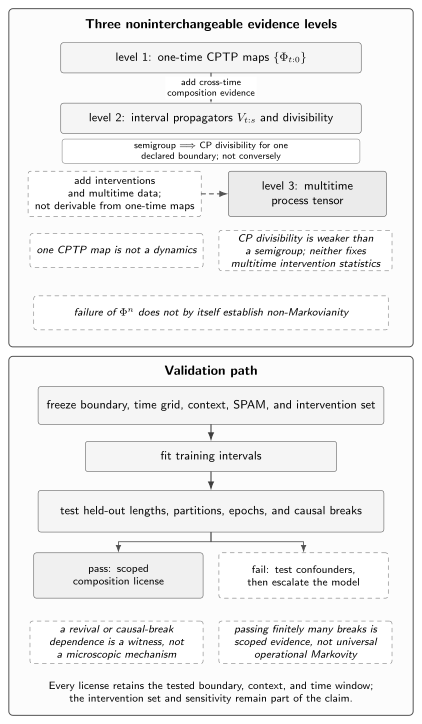
One-time physicality, interval composition, and multitime memory are different claims. Held-out intervals and causal breaks license only the tested boundary, context, time window, intervention set, and sensitivity.

Test Repeated Composition Operationally

Fit a baseline and hold out lengths

Fit the smallest model that answers the intended prediction. For a stationary-step hypothesis, estimate one $\Phi_\Delta$ from declared training sequences, freeze it, and compute $\Phi_\Delta^n$ for untouched lengths. For interval-specific evolution, fit a parsimonious family of $V_{t_{k+1}:t_k}$ and test products on reserved endpoints and nonuniform partitions. Model selection and parameter estimation must not reuse the final holdout.

Compare probabilities or reconstructed observables with their full propagated uncertainty, not merely a decay constant. A scalar residual can cancel state-dependent errors. Include preparations spanning the relevant operator space and measurements sensitive to the predicted directions. Wolf, Eisert, Cubitt, and Cirac (2008) frame the compatibility question as whether observed dynamics admit an appropriate Markovian description, rather than whether one curve looks familiar.

Randomize sequence, context, and epoch

Randomize or raster sequence lengths, preparations, contexts, and causal-break variants across acquisition time. Interleave stable references and retain timestamps. Repeat selected conditions at several epochs so time drift can be separated from sequence history. The randomization schedule and any exclusions belong in the provenance record.

Randomized benchmarking is especially sensitive to assumptions about time correlations and gate dependence. Ball et al. (2016) analyze how correlated noise changes RB behavior, while Epstein et al. (2014) examine protocol limits. Their results support diagnostic designs, not a rule that every nonexponential RB curve identifies temporal memory. Route benchmark-specific inference to Randomized Benchmarking.

Compare predictive distributions and residual structure

Choose a discrepancy before viewing the holdout: a likelihood ratio, calibrated predictive score, covariance-aware quadratic form, or task-specific risk. Compare full distributions across outcomes and contexts. Plot residuals against length, interval position, timestamp, control type, spectator state, and preceding outcome. Structure tied to clock time suggests drift; structure tied to gate identity suggests gate dependence; structure surviving a causal break suggests retained history outside the reset boundary.

Propagate shot noise, sequence sampling, calibration uncertainty, tomography covariance, and model-selection uncertainty. Predeclare the detection threshold and practical effect size. A passing model earns a bounded prediction statement for its sampled domain. A failure identifies the rejected prediction and guides the next discriminating experiment; it does not by itself name a mechanism.

Exclude Drift, Gate Dependence, Leakage, and SPAM

Drift can mimic history dependence

If long sequences are measured later than short ones, a changing dephasing rate can masquerade as length-dependent memory. If calibration is pooled across a change point, one fitted channel can also average incompatible epochs and then fail both. Proctor et al. (2020) give methods for detecting and tracking drift in quantum processors, and van Enk and Blume-Kohout (2013) show how source drift can undermine tomography assumptions.

Interleave reference sequences, preserve timestamps, compare randomized with blocked acquisition, and fit epoch-labeled alternatives. A genuine history variable should predict outcomes after clock-time and calibration effects are included. Conversely, a successful drift model is not proof that no temporal correlations remain; it merely explains the resolved discrepancy within the tested sensitivity.

Gate dependence and control distortion

A step channel inferred from one gate distribution need not transfer to another. Gate-dependent noise, frame updates, pulse overlap, coherent miscalibration, and compiler changes can make nominally equal intervals physically different. Swap gate identities while holding durations fixed, insert matched idle controls, vary compilation, and monitor pulse amplitude, detuning, and phase. Compare sequence orderings with the same gate counts.

If the residual follows gate identity or control history, replace one stationary map with schedule-labeled maps before invoking an environmental memory. RB-specific correlated and gate-dependent signatures are treated by Ball et al. (2016) and Epstein et al. (2014). A schedule-aware factorized model can still be Markovian on an enlarged classical control state.

Leakage, crosstalk, SPAM, and boundary change

Leakage stores population outside the computational model; crosstalk changes the map with spectator context; SPAM mismatch changes observed sequence endpoints; and initial correlations can invalidate a common reduced assignment. Each can make $\Phi^n$ fail without establishing a particular non-Markovian mechanism. The discriminating record is summarized below.

Candidate	Characteristic signature	Discriminating change	Required record	Falsifier or limit	Canonical owner
Retained temporal memory	Future conditional law depends on earlier history after the same system re-preparation	Insert causal breaks and vary earlier histories while fixing the future slot	Break operation, retained outcomes, replacement state, later controls, context, and uncertainty	Dependence lost after accounting for confounders; a finite null remains sensitivity-limited	What Non-Markovian Means
Drift	Residual follows timestamp, epoch, or change point more than sequence history	Randomize acquisition, interleave references, and fit epoch-labeled parameters	Shot times, calibration versions, monitors, order, and environmental record	Stable repeated epochs or held-out failure of the drift model within sensitivity	Device Characterization
Gate dependence	Residual follows gate identity or ordering at matched duration	Swap gates, compare matched idles, and balance gate counts	Compiled sequence, physical gate labels, frames, and pulse versions	Schedule-aware model fails on held-out reordered sequences	Randomized Benchmarking
Crosstalk or simultaneous context	Prediction changes with spectator state, drive, or readout activity	Toggle and randomize simultaneous operations and remote states	Spectator preparation, coupler state, concurrent pulse and readout schedule	Context labels do not predict reserved context swaps	Leakage and Crosstalk
Leakage or loss	Retained-sector trace, erasure rate, or return probability depends on length and history	Add leakage-resolving readout, vary reset, and enlarge the state space	Full outcome alphabet, acceptance, sector population, reset and return events	Enlarged-sector model still fails, or the detector cannot resolve the claimed sector	Leakage and Crosstalk
SPAM mismatch	Residual concentrates at preparation or terminal measurement and moves with boundary settings	Swap trusted preparations and measurements, interleave references, and use SPAM-aware likelihoods	Preparation commands, effects or instruments, confusion data, acceptance, and epoch	Boundary-calibrated model fails internal controls or lacks identifiability	SPAM Errors
Control distortion	Residual tracks amplitude, phase, detuning, frame, or pulse-history monitors	Insert calibrated control probes and vary pulse spacing or compensation	Waveforms, controller state, frame changes, calibration, and monitor traces	Monitored distortion cannot predict held-out controls at the required effect size	Noise Simulation
Initial correlations or boundary mismatch	Different preparation procedures do not share one reduced map	Vary reset and preparation route, add ancilla or environment bounds, and enlarge the boundary	Joint preparation assumptions, compatible domain, reset history, and retained modes	A common assignment and enlarged model predict all reserved preparations	Quantum Channels for QI

Run these alternatives as model comparisons rather than post hoc stories. Several may coexist. The aim is to determine which state variables are needed for prediction, not to force every discrepancy into a single label.

Memory Witnesses and Their Limits

Trace-distance revival is a witness

For consistently prepared states $\rho_1$ and $\rho_2$, define

$$D(t) = \frac12 \left\| \Phi_{t:0}(\rho_1-\rho_2) \right\|_1.$$

Every positive trace-preserving interval map contracts trace distance. A statistically resolved increase between $s$ and $t$ therefore falsifies P divisibility, and hence CP divisibility, for the common preparation-independent map model. Breuer, Laine, and Piilo (2009) introduced the corresponding information-backflow witness. For dephasing and the pair $|+\rangle,|-\rangle$, $D(t)=\lvert\eta(t)\rvert$, making the connection transparent.

The witness assumes comparable preparations, contexts, SPAM treatment, and uncertainty at both times. Initial correlations or a changed boundary can make the common-map premise fail. A revival identifies loss of contractivity in the tested description; it does not identify a microscopic bath or quantify every notion of memory.

Rate negativity and divisibility witnesses

An ancilla can turn lack of complete positivity of an intermediate map into an entanglement or state-distinguishability witness, as in Rivas, Huelga, and Plenio (2010). Canonical-rate negativity can provide a local divisibility witness when differentiability, invertibility, and canonical form hold. Chruściński, Kossakowski, and Rivas (2011) emphasize that divisibility and information-backflow measures are related but not universally identical.

Match the witness to the claim. Choi negativity directly rejects CP of a candidate; trace-distance revival rejects P divisibility for the stated common map; a canonical negative rate addresses a regular time-local representation. None alone certifies a complete process tensor or tells whether drift, leakage, or a boundary mismatch caused the observed violation.

Null results have finite sensitivity

No revival among finitely many state pairs and sample times does not prove CP divisibility. The optimal pair may not have been tested, a revival may lie between samples, and uncertainty can conceal a small effect. Likewise, passing finitely many causal breaks does not prove operational Markovity for interventions outside the tested span. Full certification requires an informationally complete design and a validated reconstruction with uncertainty.

Report the largest excluded discrepancy over the tested set, the temporal resolution, state and intervention coverage, confidence procedure, and model assumptions. A useful conclusion is: “No violation larger than $\epsilon$ was resolved for these pairs, intervals, contexts, and breaks.” That bounded statement can support engineering decisions without turning absence of evidence into a universal theorem.

Escalate the Model Without Overclaiming

Narrow the composition license

When a fixed-step channel passes, retain the smallest statement supported: for the named boundary and context, powers of the fitted step predict the tested preparations, observables, lengths, and tolerance. Do not promote that result automatically to arbitrary intervals or continuous time. When it fails, test interval-specific propagation, epoch labels, and schedule dependence before adding a persistent memory variable.

Validation should be prospective. Freeze parameters and thresholds, then predict new lengths, partitions, orderings, epochs, and controls. Record where the model expires and what event triggers recalibration. A narrow license is scientifically stronger than a broad adjective because it tells another reader exactly which predictions may be reused.

Enlarge the state with a memory register

If residuals depend on a finite history, carry that information explicitly. A classical hidden state can represent calibration mode, telegraph noise, controller state, or a latent fault class. A quantum enlargement can retain a resonator, leakage sector, spectator, or environmental mode. The joint update may then compose as a Markov process even though its reduced system dynamics does not.

Validate the enlarged state through interventions that alter or reset the proposed register and through held-out sequences sensitive to its predicted persistence. Multiple latent models can reproduce the same observed data, so successful prediction establishes adequacy, not unique microscopic identification. Route numerical realization and solver choices to Noise Simulation.

Escalate to a multitime model

Use the following sequence as a decision record. Each richer row must outperform the simpler alternative on reserved interventions by a predeclared criterion and retain calibrated uncertainty.

Evidence state	Next model	State carried forward	Validation intervention	Licensed prediction	Escalation trigger	Owner
Stable one-step fit	Stationary finite channel powers	Declared system state only	New equal-step lengths, preparations, and reordered sequences	Tested powers within the fixed boundary, context, and tolerance	Failure localized by length despite stable controls and epoch	This page
Schedule-dependent but factorized fit	Interval-specific channel product	System state plus known schedule label	Nonuniform partitions and unseen schedule combinations	Products of validated interval maps for declared schedules	Residual depends on more than known interval labels	This page
Context or epoch structure	Context-labeled channel family	System state plus observed context or epoch	Randomized context swaps and later epochs	Interpolation or transfer only across validated labels	Persistent residual correlates across contexts or outlives measured labels	Device Characterization
Persistent classical latent state	Hidden-state channel model	System state plus inferred classical register	Perturb, wait, or reset the proposed register and reserve long sequences	Conditional predictions for tested latent-state dynamics	Coherent or intervention-dependent residual defeats the classical model	Noise Simulation
Retained quantum mode or leakage sector	Enlarged-system CPTP dynamics	System plus explicit quantum mode or sector	Mode-selective reset, sector-resolving measurement, and entangling probes	Reduced and joint outputs for validated enlarged-state controls	Arbitrary intervention sequences remain history dependent	Leakage and Crosstalk
Intervention-dependent multitime residual	Process-tensor model	Operational temporal correlations across declared slots	Informationally complete causal breaks and held-out operation sequences	Probabilities for validated multitime interventions	New slots, contexts, or effect sizes exceed the reconstruction license	What Non-Markovian Means

A richer model is warranted by predictive necessity, not by prestige. State whether it merely fits, predicts held-out data, passes causal interventions, or supports a formal Markov condition. None of those outcomes uniquely identifies the environment without additional physical evidence.

Three Reproducible Finite Audits

Audit 1 — Exponential and Gaussian dephasing obey different laws

Set $\gamma=0.5$, $\tau=2$, $t_1=1$, and $t_2=2$. The exponential law gives $\eta_E(1)=0.6065306597126334$, $\eta_E(2)=0.36787944117144233$, and $\eta_E(1)^2=0.36787944117144233$. It therefore passes this equal-step composition check. The Gaussian law gives $\eta_G(1)=0.7788007830714049$, $\eta_G(2)=0.36787944117144233$, and $\eta_G(1)^2=0.6065306597126334$. Its semigroup defect magnitude is $0.2386512185411911$.

The two envelopes deliberately share the endpoint at $t=2$, so that endpoint cannot distinguish their laws. The Gaussian interval ratio $\eta_G(2)/\eta_G(1)=0.4723665527410147$ remains within the CPTP range. The finite calculation also evaluates $\kappa_G(t)=2t/\tau^2$ on a grid containing both endpoints. The analytic nonnegativity for every $t\geq0$ establishes CP divisibility of this family; the finite grid is a reproducibility check, not a proof about arbitrary nonexponential envelopes.

Audit 2 — A revival makes an intermediate dephasing map non-CP

Take $\eta(0)=1$, $\eta(1)=0.4$, and $\eta(2)=0.7$. Each terminal dephasing map is CPTP, but invertibility at $t_1$ fixes the interval factor to $0.7/0.4=1.75$. Constructing the normalized Choi matrix gives eigenvalues $[-0.375,0,0,1.375]$ and trace norm $1.75$. Its output partial trace is still $I/2$, so the candidate is TP but not CP.

For $|+\rangle$ and $|-\rangle$, the trace distance rises from $0.4$ at $t_1$ to $0.7$ at $t_2$, a revival of $0.3$. This rejects CP divisibility for the common preparation-independent map model under stable context and SPAM assumptions. The eigensolver and experimental thresholds must be combined before calling a negative eigenvalue resolved.

Audit 3 — Equal one-time maps hide a causal-break difference

Define $\mathcal X_r(\rho)=(1-r)\rho+rX\rho X$, so $\mathcal X_a\circ\mathcal X_b=\mathcal X_{a+b-2ab}$. Let $p=0.1$ and $q=2p(1-p)=0.18$. In model $M$, independent $E_1,E_2\sim\operatorname{Bernoulli}(p)$ give $B_1=E_1$ and $B_2=E_1\mathbin{\mathrm{xor}}E_2$. In model $C$, retained $L\sim\operatorname{Bernoulli}(p)$ and independent $C_2\sim\operatorname{Bernoulli}(q)$ give $E_1=L$, $E_2=L\mathbin{\mathrm{xor}}C_2$, $B_1=L$, and $B_2=C_2$.

In $(00,01,10,11)$ order, the cumulative joints are $[0.81,0.09,0.01,0.09]$ for $M$ and $[0.738,0.162,0.082,0.018]$ for $C$. Both have $B_1$ marginal $[0.9,0.1]$ and $B_2$ marginal $[0.82,0.18]$, so both yield $\mathcal X_p$ and $\mathcal X_q=\mathcal X_p^2$ at the two terminal times. Their joint total-variation distance is $0.144$. The cumulative covariance is $0.072$ for $M$ and zero for $C$.

After re-preparing $|0\rangle$ at $t_1$ without resetting the latent variable, model $M$ gives $\Pr(E_2=1\mid B_1=0)=\Pr(E_2=1\mid B_1=1)=0.1$. Model $C$ gives $0.18$ and $0.82$. Thus equal one-time maps and a passing fixed-power test do not fix the multitime law. The covariance reversal is deliberate: raw unconditioned covariance neither proves nor excludes operational memory, and the conditional difference does not identify a unique environment.

const tol = 1e-12;
const fail = (message) => { throw new Error(message); };
const near = (actual, expected, message) => {
  if (Math.abs(actual - expected) > tol) fail(message + `: ${actual}`);
};
const vectorNear = (actual, expected, message) => {
  if (actual.length !== expected.length) fail(message + ': length');
  actual.forEach((value, slot) => near(value, expected[slot], message));
};
const zeroMatrix = (n) => Array.from({ length: n }, () => Array(n).fill(0));
const identity = (n) => Array.from({ length: n }, (unused, row) =>
  Array.from({ length: n }, (unusedAgain, col) => Number(row === col)));
const multiply = (a, b) => a.map((row) => b[0].map((unused, col) =>
  row.reduce((sum, value, k) => sum + value * b[k][col], 0)));
const dephase = (rho, eta) => rho.map((row, r) =>
  row.map((value, c) => (r === c ? value : eta * value)));
const normalizedChoiDephasing = (eta) => {
  const choi = zeroMatrix(4);
  for (let a = 0; a < 2; a += 1) {
    for (let b = 0; b < 2; b += 1) {
      const basis = zeroMatrix(2);
      basis[a][b] = 1;
      const mapped = dephase(basis, eta);
      for (let u = 0; u < 2; u += 1) {
        for (let v = 0; v < 2; v += 1) {
          choi[2 * u + a][2 * v + b] = mapped[u][v] / 2;
        }
      }
    }
  }
  return choi;
};
const partialTraceOutput = (choi) => {
  const result = zeroMatrix(2);
  for (let a = 0; a < 2; a += 1) {
    for (let b = 0; b < 2; b += 1) {
      for (let u = 0; u < 2; u += 1) {
        result[a][b] += choi[2 * u + a][2 * u + b];
      }
    }
  }
  return result;
};
const symmetricEigenvalues = (matrix) => {
  const a = matrix.map((row) => [...row]);
  for (let sweep = 0; sweep < 100; sweep += 1) {
    let p = 0;
    let q = 1;
    let largest = 0;
    for (let r = 0; r < a.length; r += 1) {
      for (let c = r + 1; c < a.length; c += 1) {
        if (Math.abs(a[r][c]) > largest) {
          largest = Math.abs(a[r][c]);
          p = r;
          q = c;
        }
      }
    }
    if (largest < tol / 100) break;
    const app = a[p][p];
    const aqq = a[q][q];
    const apq = a[p][q];
    const angle = Math.atan2(2 * apq, aqq - app) / 2;
    const c = Math.cos(angle);
    const s = Math.sin(angle);
    for (let k = 0; k < a.length; k += 1) {
      if (k === p || k === q) continue;
      const akp = a[k][p];
      const akq = a[k][q];
      a[k][p] = c * akp - s * akq;
      a[p][k] = a[k][p];
      a[k][q] = s * akp + c * akq;
      a[q][k] = a[k][q];
    }
    a[p][p] = c * c * app - 2 * s * c * apq + s * s * aqq;
    a[q][q] = s * s * app + 2 * s * c * apq + c * c * aqq;
    a[p][q] = 0;
    a[q][p] = 0;
  }
  return a.map((row, slot) => row[slot]).sort((x, y) => x - y);
};
const checkTp = (choi, message) => {
  const reduced = partialTraceOutput(choi);
  vectorNear(reduced.flat(), [0.5, 0, 0, 0.5], message);
};
const checkCp = (choi, message) => {
  if (symmetricEigenvalues(choi)[0] < -tol) fail(message);
};

const gamma = 0.5;
const tau = 2;
const t1 = 1;
const t2 = 2;
const etaExp = (t) => Math.exp(-gamma * t);
const etaGaussian = (t) => Math.exp(-((t / tau) ** 2));
near(etaExp(t1), 0.6065306597126334, 'exponential first time');
near(etaExp(t2), 0.36787944117144233, 'exponential second time');
near(etaExp(t1) ** 2, etaExp(t2), 'exponential equal steps');
near(etaGaussian(t1), 0.7788007830714049, 'Gaussian first time');
near(etaGaussian(t2), 0.36787944117144233, 'Gaussian second time');
near(etaGaussian(t1) ** 2, 0.6065306597126334, 'Gaussian equal-step prediction');
near(Math.abs(etaGaussian(t1) ** 2 - etaGaussian(t2)),
  0.2386512185411911, 'Gaussian semigroup defect');
near(etaGaussian(t2) / etaGaussian(t1),
  0.4723665527410147, 'Gaussian interval ratio');
near(etaExp(t2), etaGaussian(t2), 'shared endpoint');
const rateGrid = [0, 0.25, 0.5, 1, 1.5, 2];
rateGrid.forEach((t) => {
  const rate = 2 * t / (tau ** 2);
  if (rate < -tol) fail('negative Gaussian canonical rate');
});

const endpointEtas = [1, 0.4, 0.7];
endpointEtas.forEach((eta) => {
  const choi = normalizedChoiDephasing(eta);
  checkCp(choi, 'endpoint is not CP');
  checkTp(choi, 'endpoint is not TP');
});
const intervalRatio = endpointEtas[2] / endpointEtas[1];
near(intervalRatio, 1.75, 'revival interval ratio');
const intervalChoi = normalizedChoiDephasing(intervalRatio);
const intervalSpectrum = symmetricEigenvalues(intervalChoi);
vectorNear(intervalSpectrum, [-0.375, 0, 0, 1.375], 'interval spectrum');
near(intervalSpectrum.reduce((sum, value) => sum + Math.abs(value), 0),
  1.75, 'interval trace norm');
checkTp(intervalChoi, 'intermediate candidate is not TP');
if (intervalSpectrum[0] >= -tol) fail('intermediate candidate unexpectedly CP');
const plus = [[0.5, 0.5], [0.5, 0.5]];
const minus = [[0.5, -0.5], [-0.5, 0.5]];
const subtract = (a, b) => a.map((row, r) => row.map((value, c) => value - b[r][c]));
const traceDistanceRealQubit = (a, b) => symmetricEigenvalues(subtract(a, b))
  .reduce((sum, value) => sum + Math.abs(value), 0) / 2;
const distance1 = traceDistanceRealQubit(dephase(plus, 0.4), dephase(minus, 0.4));
const distance2 = traceDistanceRealQubit(dephase(plus, 0.7), dephase(minus, 0.7));
near(distance1, 0.4, 'first trace distance');
near(distance2, 0.7, 'second trace distance');
near(distance2 - distance1, 0.3, 'trace-distance revival');

const p = 0.1;
const q = 2 * p * (1 - p);
near(q, 0.18, 'composed bit-flip probability');
const bernoulli = (value, probability) => (value === 1 ? probability : 1 - probability);
const jointM = [0, 0, 0, 0];
const jointC = [0, 0, 0, 0];
const primitiveM = [];
const primitiveC = [];
for (const e1 of [0, 1]) {
  for (const e2 of [0, 1]) {
    const probability = bernoulli(e1, p) * bernoulli(e2, p);
    const b1 = e1;
    const b2 = e1 ^ e2;
    jointM[2 * b1 + b2] += probability;
    primitiveM.push({ b1, e2, probability });
  }
}
for (const latent of [0, 1]) {
  for (const fresh of [0, 1]) {
    const probability = bernoulli(latent, p) * bernoulli(fresh, q);
    const b1 = latent;
    const b2 = fresh;
    const e2 = latent ^ fresh;
    jointC[2 * b1 + b2] += probability;
    primitiveC.push({ b1, e2, probability });
  }
}
vectorNear(jointM, [0.81, 0.09, 0.01, 0.09], 'model M joint');
vectorNear(jointC, [0.738, 0.162, 0.082, 0.018], 'model C joint');
const marginal = (joint, bit) => {
  const result = [0, 0];
  joint.forEach((probability, slot) => {
    const value = bit === 1 ? Math.floor(slot / 2) : slot % 2;
    result[value] += probability;
  });
  return result;
};
vectorNear(marginal(jointM, 1), [0.9, 0.1], 'M first marginal');
vectorNear(marginal(jointC, 1), [0.9, 0.1], 'C first marginal');
vectorNear(marginal(jointM, 2), [0.82, 0.18], 'M second marginal');
vectorNear(marginal(jointC, 2), [0.82, 0.18], 'C second marginal');
const totalVariation = jointM.reduce((sum, value, slot) =>
  sum + Math.abs(value - jointC[slot]), 0) / 2;
near(totalVariation, 0.144, 'joint total variation');
const covariance = (joint) => {
  let first = 0;
  let second = 0;
  let product = 0;
  joint.forEach((probability, slot) => {
    const b1 = Math.floor(slot / 2);
    const b2 = slot % 2;
    first += probability * b1;
    second += probability * b2;
    product += probability * b1 * b2;
  });
  return product - first * second;
};
near(covariance(jointM), 0.072, 'M covariance');
near(covariance(jointC), 0, 'C covariance');
const conditionalFault = (primitive, prior) => {
  const selected = primitive.filter((event) => event.b1 === prior);
  const mass = selected.reduce((sum, event) => sum + event.probability, 0);
  return selected.reduce((sum, event) => sum + event.probability * event.e2, 0) / mass;
};
near(conditionalFault(primitiveM, 0), 0.1, 'M future after prior zero');
near(conditionalFault(primitiveM, 1), 0.1, 'M future after prior one');
near(conditionalFault(primitiveC, 0), 0.18, 'C future after prior zero');
near(conditionalFault(primitiveC, 1), 0.82, 'C future after prior one');
const bitFlip = (rho, probability) => {
  const x = [[0, 1], [1, 0]];
  const flipped = multiply(multiply(x, rho), x);
  return rho.map((row, r) => row.map((value, c) =>
    (1 - probability) * value + probability * flipped[r][c]));
};
const basisOperators = [
  [[1, 0], [0, 0]],
  [[0, 1], [0, 0]],
  [[0, 0], [1, 0]],
  [[0, 0], [0, 1]],
];
basisOperators.forEach((basis) => {
  vectorNear(bitFlip(bitFlip(basis, p), p).flat(),
    bitFlip(basis, q).flat(), 'bit-flip composition');
});
console.log('Markovian/non-Markovian finite audits: PASS');

Canonical Owners and Common Claim Failures

This page owns the QI-facing validation crosswalk from finite channels to fixed powers, interval products, semigroups, CP divisibility, causal breaks, and model escalation. The broad mechanism taxonomy belongs to Noise in Quantum Information, explicit channel cards to Common Noise Models, and the $T_1$–$T_2$ crosswalk to Dephasing and Amplitude Damping. Formal definitions belong to What Non-Markovian Means, CP Divisibility, Information Backflow, and Non-Markovianity Measures. Microscopic constructions belong to Collision Models and Memory Kernels.

Experimental reconstruction and model selection belong to Process Tomography and Device Characterization; simulator implementation belongs to Noise Simulation. Error Mitigation Overview owns cross-family estimator selection and shared resource ledgers. Zero-Noise Extrapolation owns method-specific physical scaling laws, calibrated effective gains, and coordinate-zero intercept inference. This page retains semigroup, generator, memory, intervention, model-selection, and falsification scope, while the chapter guide preserves the broader learning path.

Keep conclusions at the rung actually tested: “the fixed-step model failed,” “the tested intermediate map was non-CP,” “trace distance revived for this pair,” “a causal-break conditional changed,” or “the selected multitime model predicted held-out data.” None of these sentences entails the others without added evidence.

Calling one CPTP map a dynamics. Physicality at one endpoint supplies no law across times. State exactly which map was reconstructed and what additional interval or sequence evidence is absent.

Equating fixed-power failure with non-Markovianity. A failed $\Phi^n$ prediction rejects stationary repeated use. Test time dependence, context, drift, gate dependence, leakage, SPAM, and boundary changes before assigning retained memory.

Equating semigroup failure with CP-indivisibility. A Gaussian dephasing envelope is the counterexample: it has a nonnegative canonical rate and CPTP interval factors while failing time homogeneity.

Defining divisibility through an inverse. Inversion is a convenience only for invertible maps. At singular times solve the existence and extension problem on the image, with physicality and uncertainty constraints.

Checking Choi positivity but not TP. A candidate interval map must satisfy both positive semidefiniteness and the declared partial-trace condition. Numerical projection changes the estimate and must never replace a reported failure.

Treating a witness as a mechanism. Choi negativity, trace-distance revival, or causal-break dependence rejects a specified model under stated assumptions. It does not uniquely identify the environment.

Promoting a finite null result to universal Markovity. Report tested pairs, intervals, interventions, contexts, and detectable effect size. Untested temporal slots and operations remain outside the license.

Exercises

1. Classify six composition claims

For each of the following, state what it predicts and the evidence needed for the next rung: one CPTP $\Phi_{t:0}$; a CPTP family $\{\Phi_{t:0}\}$; interval products; fixed-step powers; CP divisibility; and a time-homogeneous semigroup.

Solution

One CPTP map predicts terminal outputs at one declared boundary and time. Additional terminal tomography gives a family, but cross-time compatibility still needs explicit factorization tests. Interval products predict terminal maps from ordered interval-specific channels; equality of all equal-duration factors and held-out powers is needed for a stationary fixed-step claim. Fixed powers remain discrete, so nonuniform times, $\Phi_0=\operatorname{id}$, time homogeneity, continuity, and generator consistency are needed for a semigroup.

CP divisibility instead requires a CPTP $V_{t:s}$ for every claimed pair, verified by both Choi positivity and TP. It is broader than a semigroup and does not determine intervention statistics. A semigroup implies CP divisibility under the common boundary but likewise does not establish the operational process condition. That final question requires causal breaks or a complete multitime reconstruction. At every rung, failure conditions include changed spaces, preparation dependence, context mismatch, and uncertainty larger than the tested discrepancy; the formal next-step owners are CP Divisibility and What Non-Markovian Means.

2. Separate semigroup failure from CP-indivisibility

Derive the composition laws for $\eta_E(t)=e^{-\gamma t}$ and $\eta_G(t)=e^{-(t/\tau)^2}$. Prove the Gaussian family is CP-divisible for $t\geq0$ and explain the scope of the conclusion.

Solution

Because dephasing factors multiply, $\mathcal D_{\eta(t)}\mathcal D_{\eta(s)}=\mathcal D_{\eta(t)\eta(s)}$. The exponential obeys $e^{-\gamma(t+s)}=e^{-\gamma t}e^{-\gamma s}$ and is therefore a semigroup. For the Gaussian,

$$\frac{\eta_G(t)}{\eta_G(s)} = \exp\!\left[-\frac{t^2-s^2}{\tau^2}\right], \qquad t\geq s\geq0,$$

which lies in $(0,1]$. Hence every interval factor defines a CPTP dephasing map, equivalently $\kappa_G(t)=2t/\tau^2\geq0$. Yet $\eta_G(t+s)$ contains $2st/\tau^2$ and does not equal the product for positive $s,t$.

Thus this family is CP-divisible but not a semigroup. The proof assumes the declared qubit dephasing family for all nonnegative times; it does not say that every nonexponential decay is CP-divisible or that multitime interventions are Markov. Generator theorems and their hypotheses belong to Quantum Dynamical Semigroups.

3. Construct and Choi-test an intermediate propagator

For $\eta(0)=1$, $\eta(1)=0.4$, and $\eta(2)=0.7$, construct the normalized Choi matrices of the endpoint maps and the unique interval candidate. Explain how a singular earlier map changes the workflow.

Solution

For dephasing factor $r$ in the declared output–input tensor order,

$$J_N(\mathcal D_r) = \frac12 \begin{pmatrix} 1&0&0&r\\ 0&0&0&0\\ 0&0&0&0\\ r&0&0&1 \end{pmatrix}.$$

Its eigenvalues are $(1-r)/2$, $0$, $0$, and $(1+r)/2$, and its output partial trace is $I/2$. The endpoint values $1$, $0.4$, and $0.7$ therefore give CPTP maps. Invertibility at the earlier nonzero factor makes the interval candidate unique, with $r=0.7/0.4=1.75$ and spectrum $[-0.375,0,0,1.375]$. It is TP but not CP beyond numerical and statistical tolerance.

If the earlier factor were zero, the quotient would be undefined. One must solve for a CPTP extension satisfying the factorization on the earlier map’s image; it may be nonunique or nonexistent. A pseudoinverse is not a physicality proof. CP Divisibility owns the general Choi feasibility treatment.

4. Relate a revival to trace-distance backflow

Evolve $|+\rangle$ and $|-\rangle$ under the revival fixture, derive their trace distance, and state both the licensed witness and its caveats.

Solution

Their density-matrix difference is

$$\rho_+-\rho_- = \begin{pmatrix}0&1\\1&0\end{pmatrix}.$$

Dephasing multiplies its off-diagonal entries by $\eta(t)$, producing eigenvalues $\pm\eta(t)$. Half the trace norm is therefore $D(t)=\lvert\eta(t)\rvert$. The fixture gives $D(t_1)=0.4$, $D(t_2)=0.7$, and revival $0.3$. A positive TP propagator would contract this distance, so the resolved revival rejects P divisibility and hence CP divisibility for the common preparation-independent reduced-map model.

The claim requires consistent preparation of both states, the same system boundary and context, SPAM-aware uncertainty, and temporal resolution adequate to resolve the increase. Initial correlations or drift can invalidate the common-map comparison. The result is an information-backflow witness in the sense of Breuer, Laine, and Piilo, not identification of a bath or a universal measure; Information Backflow owns that formal development.

5. Distinguish equal one-time maps by a causal break

Construct models $M$ and $C$ from Audit 3. Derive their terminal maps, joint laws, and causal-break conditionals, and say what re-preparing the system does not reset.

Solution

Independent Bernoulli increments in $M$ give $B_1=E_1$ with error $p$ and $B_2=E_1\mathbin{\mathrm{xor}}E_2$ with error $q=2p(1-p)$. Enumerating $(E_1,E_2)$ gives $[0.81,0.09,0.01,0.09]$. In $C$, independent $(L,C_2)$ with probabilities $(p,q)$ directly give $(B_1,B_2)=(L,C_2)$ and joint $[0.738,0.162,0.082,0.018]$. Thus both terminal channels are $\mathcal X_p$ and $\mathcal X_q=\mathcal X_p^2$, although their joint laws differ by total variation $0.144$.

After a system replacement at $t_1$, $M$ has future fault $E_2$ independent of $B_1$, giving $0.1$ in either branch. In $C$, $E_2=L\mathbin{\mathrm{xor}}C_2$, so conditioning on $L=B_1$ gives $0.18$ and $0.82$. Re-preparation discards the system state but does not reset $L$ or an analogous environment. The evidence distinguishes the two processes; it neither identifies a unique latent mechanism nor transfers beyond the tested break operations. The process-tensor owner is What Non-Markovian Means.

6. Diagnose a failed fixed-channel prediction

Design separate tests for drift, gate dependence, control distortion, crosstalk, leakage, SPAM, and initial-correlation or boundary mismatch before assigning retained memory.

Solution

Randomize lengths across timestamped epochs and interleave references to test drift. At matched duration and gate count, swap gate identities and orderings for gate dependence; add calibrated idle and pulse-monitor variants for control distortion. Toggle spectator preparations and simultaneous operations for crosstalk. Retain erasure and leakage-resolving outcomes, vary reset, and fit an enlarged sector model for leakage. Swap trusted preparations and measurements and use a SPAM-aware likelihood for boundary error. Finally vary reset and preparation routes, bound initial correlations, and enlarge the system with a suspected retained mode.

Each alternative needs a predeclared signature, held-out condition, uncertainty, and falsifier. If one context-labeled factorized model predicts the reserved data, the license is that model’s domain—not universal absence of memory. If causal-break dependence survives these controls, retained temporal information is supported for the named boundary and intervention set. Route acquisition and model selection to Device Characterization and numerical enlargement to Noise Simulation.

7. Design a randomized held-out memory study

Design a timestamped study with nonuniform interval partitions, causal breaks, contexts, uncertainty, versioned provenance, explicit falsifiers, and a model-escalation rule.

Solution

Freeze system and enlarged sectors, preparation and SPAM models, time grid, schedule, contexts, compiler and calibration versions, allowed interventions, and the effect size of interest. Randomize equal and nonuniform partitions, preparations, spectator conditions, and causal-break histories across time; interleave reference sequences and retain shot-level timestamps and outcomes. Use training data to choose a baseline, a separate validation set to choose complexity, and untouched lengths, partitions, epochs, and break sequences for the final predictive test.

Propagate shot, tomography, calibration, and model-selection uncertainty. Predeclare distributional discrepancy, confidence rule, multiplicity treatment, and separate falsifiers for stationarity, interval factorization, drift, context dependence, hidden-state persistence, and causal-break independence. Escalate from one channel to interval-specific or context-labeled maps, then to a validated latent or enlarged-system state, and finally to a process tensor only when reserved interventions require it.

The final report gives versions and hashes, exclusions, sensitivity, rejected alternatives, and an expiry trigger. A defensible pass says only that the selected model predicted the named holdouts within tolerance; a failure names the rejected claim and next test, not an assumed mechanism.

References

• H. Ball, T. M. Stace, S. T. Flammia, and M. J. Biercuk, “Effect of noise correlations on randomized benchmarking,” Physical Review A 93, 022303 (2016), doi:10.1103/PhysRevA.93.022303.
• H.-P. Breuer, E.-M. Laine, and J. Piilo, “Measure for the degree of non-Markovian behavior of quantum processes in open systems,” Physical Review Letters 103, 210401 (2009), doi:10.1103/PhysRevLett.103.210401.
• H.-P. Breuer, E.-M. Laine, J. Piilo, and B. Vacchini, “Colloquium: Non-Markovian dynamics in open quantum systems,” Reviews of Modern Physics 88, 021002 (2016), doi:10.1103/RevModPhys.88.021002.
• D. Chruściński, A. Kossakowski, and Á. Rivas, “Measures of non-Markovianity: Divisibility versus backflow of information,” Physical Review A 83, 052128 (2011), doi:10.1103/PhysRevA.83.052128.
• D. Chruściński, Á. Rivas, and E. Størmer, “Divisibility and information flow notions of quantum Markovianity for noninvertible dynamical maps,” Physical Review Letters 121, 080407 (2018), doi:10.1103/PhysRevLett.121.080407.
• J. M. Epstein, A. W. Cross, E. Magesan, and J. M. Gambetta, “Investigating the limits of randomized benchmarking protocols,” Physical Review A 89, 062321 (2014), doi:10.1103/PhysRevA.89.062321.
• V. Gorini, A. Kossakowski, and E. C. G. Sudarshan, “Completely positive dynamical semigroups of $N$-level systems,” Journal of Mathematical Physics 17, 821–825 (1976), doi:10.1063/1.522979.
• G. Lindblad, “On the generators of quantum dynamical semigroups,” Communications in Mathematical Physics 48, 119–130 (1976), doi:10.1007/BF01608499.
• F. A. Pollock, C. Rodríguez-Rosario, T. Frauenheim, M. Paternostro, and K. Modi, “Non-Markovian quantum processes: Complete framework and efficient characterization,” Physical Review A 97, 012127 (2018), doi:10.1103/PhysRevA.97.012127.
• F. A. Pollock, C. Rodríguez-Rosario, T. Frauenheim, M. Paternostro, and K. Modi, “Operational Markov condition for quantum processes,” Physical Review Letters 120, 040405 (2018), doi:10.1103/PhysRevLett.120.040405.
• T. Proctor, M. Revelle, E. Nielsen, K. Rudinger, D. Lobser, P. Maunz, R. Blume-Kohout, and K. Young, “Detecting and tracking drift in quantum information processors,” Nature Communications 11, 5396 (2020), doi:10.1038/s41467-020-19074-4.
• Á. Rivas, S. F. Huelga, and M. B. Plenio, “Entanglement and non-Markovianity of quantum evolutions,” Physical Review Letters 105, 050403 (2010), doi:10.1103/PhysRevLett.105.050403.
• S. J. van Enk and R. Blume-Kohout, “When quantum tomography goes wrong: drift of quantum sources and other errors,” New Journal of Physics 15, 025024 (2013), doi:10.1088/1367-2630/15/2/025024.
• M. M. Wolf, J. Eisert, T. S. Cubitt, and J. I. Cirac, “Assessing non-Markovian quantum dynamics,” Physical Review Letters 101, 150402 (2008), doi:10.1103/PhysRevLett.101.150402.