Dephasing and Amplitude Damping

A coherence time becomes a channel parameter only after the experiment that produced it has been frozen. This page gives a reproducible crosswalk from protocol-qualified longitudinal relaxation, transverse coherence, and equilibrium-population records to one finite-time phase-covariant qubit channel. The workflow fixes the energy basis and retained subspace, converts the record without counting relaxation twice, translates among density-matrix, Bloch-affine, Pauli-transfer, Kraus, and Choi descriptions, composes scheduled idles in circuit order, and checks held-out population and coherence predictions. It does not infer a bath Hamiltonian, a noise spectrum, or a universal Markov model from a decay curve.

Required background. Quantum Channels for QI supplies the column Pauli-transfer and affine conventions, representation translation, composition order, and finite physicality checks. Dephasing versus Dissipation supplies the population-versus-coherence distinction and the energy-basis language used here without rederiving open-system dynamics.

Helpful background. Common Noise Models supplies the broader model-card and parameter ledger. Metrics for Quantum Hardware supplies protocol, fit-law, uncertainty, and validity-interval reporting.

Dephasing and Relaxation as Distinct Channel Geometry

Population flow and transverse coherence

Fix the ordered energy basis before naming any decay parameter:

$$\lvert0\rangle=\text{lower-energy state}, \qquad \lvert1\rangle=\text{upper-energy state},$$ $$\rho=\frac{I+xX+yY+zZ}{2}, \qquad \rho_{01}=\frac{x-iy}{2}, \qquad z=\rho_{00}-\rho_{11}.$$

Longitudinal relaxation changes the energy populations and generally translates the Bloch vector toward a thermal fixed point. Dephasing suppresses the off-diagonal element in this basis without, by itself, changing those populations. Bloch’s phenomenological equations already separate longitudinal and transverse relaxation, while Breuer and Petruccione give the modern open-system formulation. This page uses that separation as an input convention; the physical distinction and its limits remain at the prerequisite owner.

For one declared interval, the most useful phase-covariant map is

$$\rho_{11}'=\eta\rho_{11}+(1-\eta)n_{\mathrm{eq}}, \qquad \rho_{01}'=c\rho_{01}.$$

Here $0\leq\eta\leq1$ is the surviving population difference, $n_{\mathrm{eq}}$ is the equilibrium excited-state population, and $c$ is a complex coherence factor. The map separates population contraction, fixed-point translation, transverse contraction, and coherent phase. Those four features are experimentally distinguishable and should not be collapsed into one “decoherence rate.”

Timescale labels are protocol summaries

A reported $T_1$, $T_2$, or $T_2^*$ is the parameter of a stated fit, not a self-sufficient property of an abstract qubit. Ramsey’s separated-oscillatory-field method and Hahn’s echo sequence establish different experimental sensitivities. Modern analyses by Ithier and collaborators show how control sequence, noise spectrum, and device operating point enter observed decay. Even the word “exponential” is a model choice: an envelope can instead be Gaussian, stretched exponential, multi-exponential, oscillatory, or interrupted by drift.

The record must therefore include the preparation and readout convention, pulse sequence, rotating frame, fit function, fit window, uncertainty, and epoch. A Ramsey $T_2^*$ is ordinarily sensitive to slowly varying detuning that an echo suppresses. An echo time and a longer dynamical-decoupling time probe different filtered bands. Degen, Reinhard, and Cappellaro review this filter-dependent viewpoint for quantum sensing; Bylander and collaborators demonstrate it in superconducting-qubit noise spectroscopy. These sources support protocol dependence, not permission to infer a unique spectrum from one fitted number.

What this page owns

The output here is a finite, testable channel record for a retained two-level system at a named circuit location. Dephasing Channel owns the formal phase-flip and phase-damping channel definitions, environment-record and random-phase pictures, higher-dimensional extension, and formal semigroup limit. Amplitude-Damping Channel owns the zero-temperature definition, dilation, fixed point, and formal thermal extension. Kraus, Choi, and Stinespring Views owns minimal realizations and Kraus freedom.

The master-equation leaves own generator derivations and rate conventions; Metrics for Quantum Hardware owns how $T_1$, $T_2$, and state occupancy are acquired and reported; Noise Simulation owns scalable scheduling and sampling algorithms. The narrower task here is conversion, physicality, composition, prediction, and falsification. Nielsen and Chuang and Watrous provide the general channel framework used for those finite checks, but no representation conversion alone establishes a microscopic mechanism.

Freeze the Coherence-Time Record

Energy basis, retained subspace, and equilibrium state

Record which pair of physical levels is called $\lvert0\rangle,\lvert1\rangle$ and whether population outside that pair is discarded, postselected, or represented explicitly. A trace-preserving qubit channel is inappropriate if appreciable leakage leaves the retained subspace without a return or flag model. Also specify whether readout labels have been corrected for assignment error and whether the stated ground and excited preparations are physical preparations or fitted endpoints.

Define

$$n_{\mathrm{eq}}:=\rho_{11}^{(\mathrm{eq})}, \qquad z_{\mathrm{eq}}:=1-2n_{\mathrm{eq}}.$$

This convention makes $z_{\mathrm{eq}}=1$ at zero temperature and $z_{\mathrm{eq}}=0$ for an equally populated doublet. A residual excited-state population may reflect a thermal distribution, nonequilibrium quasiparticles, imperfect reset, readout bias, or leakage. Calling it a temperature requires additional calibration and a licensed equilibrium model. Makhlin, Schön, and Shnirman discuss relaxation and dephasing in solid-state qubits while emphasizing their device dependence.

Pulse sequence, fit law, window, and uncertainty

Freeze the inversion-recovery sequence used for $T_1$ and the Ramsey, echo, or decoupling sequence used for transverse coherence. State whether the fitted population is $A e^{-t/T_1}+B$, a thermal recovery about $n_{\mathrm{eq}}$, or another law. For transverse data, retain both quadratures when available and record any fitted detuning. If the complex envelope is $c(t)=W(t)e^{-i\theta(t)}$, the magnitude and phase are separate observables.

The fit window matters because a local exponential can summarize a nonexponential curve over a restricted interval. Report confidence intervals or posterior uncertainty, residual structure, number of repetitions, and any preprocessing. Do not combine a $T_1$ measured in one epoch with a $T_2$ measured after recalibration without labeling that assumption. Cywiński and collaborators show explicitly how pulse sequences reshape dephasing under low-frequency noise, so a fit parameter cannot be transported across sequences merely because its units are time.

Interval, circuit placement, context, and validation target

Name the channel interval $\Delta t$: an idle between two gates, a measurement latency, a reset wait, or another scheduled segment. State whether the map is placed before or after a basis-changing ideal gate and which frame defines $X$ and $Y$. Record simultaneous activity, spectator state, control amplitudes, temperature, calibration epoch, and any conditioning variables. These details determine whether one parameter set can be reused.

Finally, name the held-out claim before fitting: perhaps $P(1\mid0)$ and $P(1\mid1)$ at unused times, both Ramsey quadratures, or an idle fidelity after an explicitly modeled virtual-$Z$ correction. A bare time constant has no such prediction contract. The figure summarizes the conversion path and the three cautions that must remain visible throughout it.

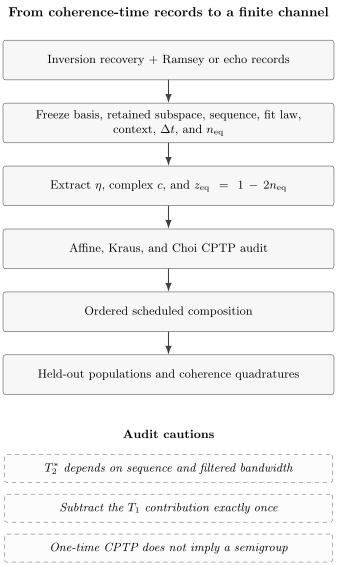
A protocol-qualified record becomes a finite channel only after basis, subspace, sequence, fit, context, interval, and fixed point are frozen. The physicality and composition audits do not upgrade a one-time fit into a semigroup.

Dephasing Convention Crosswalk

Complex coherence factor

Write the measured finite-time factor as

$$c=|c|e^{-i\theta}, \qquad \rho_{01}'=c\rho_{01}.$$

The magnitude $|c|$ is the total transverse contraction over the declared interval. The phase $\theta$ is a coherent $Z$-axis frame rotation in the stated sign convention. If a detuning or virtual-$Z$ correction removes it, report both the raw and corrected predictions; do not silently replace $\operatorname{Re}c$ by $|c|$. The phase convention is fixed by $\rho_{01}=(x-iy)/2$: positive $\theta$ yields the transverse matrix used below, not its transpose.

A standalone dephasing factor $\lambda_\phi$ describes only the part remaining after relaxation-induced coherence loss has been removed. In the matched Markov model it is real and nonnegative. A measured negative or complex factor can still define a finite channel, but then it includes a coherent phase or a sign reversal and should not be forced into a stochastic phase-flip probability without declaring the extra unitary.

Phase-flip and phase-damping parameters

For real $0\leq\lambda_\phi\leq1$, the stochastic phase-flip ledger is

$$\mathcal Z_{p_Z}(\rho) =(1-p_Z)\rho+p_ZZ\rho Z, \qquad \lambda_\phi=1-2p_Z, \qquad p_Z=\frac{1-\lambda_\phi}{2}.$$

An alternative phase-damping ledger uses

$$g=1-\lambda_\phi^2, \qquad \lambda_\phi=\sqrt{1-g}.$$

Complete dephasing is $\lambda_\phi=0$, so $p_Z=1/2$ and $g=1$. The endpoint $p_Z=1$ is instead the unitary $Z$ channel: it preserves the magnitude of coherence and reverses its sign. Confusing those endpoints is a common consequence of calling every displayed parameter “dephasing probability.” The formal dephasing owner derives the corresponding Kraus and Choi forms; this page uses the ledgers only to translate a qualified finite factor.

Markovian rate and nonexponential envelope

Under an exponential pure-dephasing model,

$$\lambda_\phi(t)=e^{-t/T_\phi}.$$

That formula licenses multiplicative composition only when the same time-homogeneous, memoryless model applies across the composed intervals. A measured envelope $W(t)$ can define a CPTP dephasing map at each sampled time whenever $|W(t)|\leq1$, yet fail $W(t+s)=W(t)W(s)$. Gaussian quasistatic decay is the principal fixture below. A stretched exponential $e^{-(t/\tau)^\beta}$ is multiplicative only for $\beta=1$.

Gorini, Kossakowski, and Sudarshan and, independently, Lindblad characterize generators of quantum dynamical semigroups. Their results justify exponential composition under their assumptions; they do not make every finite CPTP fit divisible. This distinction is why the phrase time-indexed family is used for a collection of one-time maps whose cross-time law has not been established.

quantity	symbol	protocol or definition	channel role	allowed range or licensed condition	common failure
longitudinal relaxation time	$T_1$	qualified population-recovery fit	sets $\eta$ in an exponential model	$T_1>0$ for that fit and context	treated as a context-free constant
homogeneous transverse time	$T_2$	qualified exponential echo or homogeneous fit	sets total $\lvert c\rvert$	$T_2>0$; sequence must be named	confused with Ramsey $T_2^*$
Ramsey inhomogeneous time	$T_2^*$	Ramsey envelope with stated fit law	summarizes Ramsey coherence	protocol and bandwidth dependent	substituted for another sequence
pure-dephasing time	$T_\phi$	$T_\phi^{-1}=T_2^{-1}-(2T_1)^{-1}$	sets additional $\lambda_\phi$	matched exponential Markov model	inferred when the rate difference is negative
population-difference survival	$\eta$	$e^{-\Delta t/T_1}$ or finite fit	contracts $z-z_{\mathrm{eq}}$	$0\leq\eta\leq1$ here	confused with relaxation probability
relaxation probability	$\gamma$	$1-\eta$	weights thermal jumps	$0\leq\gamma\leq1$	used as an amplitude rather than a probability
equilibrium excited population	$n_{\mathrm{eq}}$	qualified long-time population	fixes affine translation	$0\leq n_{\mathrm{eq}}\leq1$	called a temperature without evidence
complex coherence factor	$c$	ratio $\rho_{01}'/\rho_{01}$	contracts and rotates $x,y$	exact Choi bound below	phase discarded without a correction
pure-dephasing factor	$\lambda_\phi$	$\lvert c\rvert/\sqrt\eta$ in matched model	adds dephasing beyond relaxation	$0\leq\lambda_\phi\leq1$ in that model	relaxation contribution counted twice
phase-flip probability	$p_Z$	$(1-\lambda_\phi)/2$	stochastic-$Z$ ledger	$0\leq p_Z\leq1/2$ for nonnegative contraction	$p_Z=1$ called complete dephasing
phase-damping parameter	$g$	$1-\lambda_\phi^2$	environment-record ledger	$0\leq g\leq1$	identified numerically with $p_Z$

Zero- and Finite-Temperature Amplitude Damping

Zero-temperature amplitude damping

At zero temperature the equilibrium excited population is $n_{\mathrm{eq}}=0$. With $\gamma=1-\eta$, the usual two-Kraus channel is

$$A_0=\begin{pmatrix}1&0\\0&\sqrt\eta\end{pmatrix}, \qquad A_1=\begin{pmatrix}0&\sqrt\gamma\\0&0\end{pmatrix}.$$

It sends $\rho_{11}\mapsto\eta\rho_{11}$ and $\rho_{01}\mapsto\sqrt\eta\rho_{01}$. Thus relaxation alone contributes half its population-decay rate to transverse decay. The channel is nonunital because it translates every state toward $\lvert0\rangle$. It is not a Pauli channel and should not be simulated as a random $X$ event: a jump probability depends on the state, and the no-jump branch also changes amplitudes.

Use this zero-temperature form only when upward excitation is negligible for the stated interval and validation precision. A nonzero stationary excited population is direct evidence that the two-Kraus fixed point is wrong, even if the early-time decay of an initially excited state looks approximately exponential.

Upward and downward thermal rates

For a Markovian two-level thermal-rate model, define

$$\Gamma_1=\Gamma_\downarrow+\Gamma_\uparrow, \qquad T_1=\Gamma_1^{-1}, \qquad n_{\mathrm{eq}}= \frac{\Gamma_\uparrow}{\Gamma_\downarrow+\Gamma_\uparrow}.$$

The finite interval has

$$\eta=e^{-\Delta t/T_1}, \qquad \gamma=1-\eta.$$

Upward and downward rates determine the fixed point as well as the approach rate. If only $T_1$ is reported, their sum is known but their ratio is not. Conversely, $T_1$ together with a qualified $n_{\mathrm{eq}}$ determines $\Gamma_\uparrow=n_{\mathrm{eq}}/T_1$ and $\Gamma_\downarrow=(1-n_{\mathrm{eq}})/T_1$ within this model. Detailed-balance or effective-temperature interpretations belong to the thermal master-equation owner and require an equilibrium assumption.

Generalized amplitude damping and its fixed state

An ordered Kraus family with the required fixed point is

$$\begin{aligned} A_0&=\sqrt{1-n_{\mathrm{eq}}} \begin{pmatrix}1&0\\0&\sqrt\eta\end{pmatrix}, & A_1&=\sqrt{1-n_{\mathrm{eq}}} \begin{pmatrix}0&\sqrt\gamma\\0&0\end{pmatrix},\\ A_2&=\sqrt{n_{\mathrm{eq}}} \begin{pmatrix}\sqrt\eta&0\\0&1\end{pmatrix}, & A_3&=\sqrt{n_{\mathrm{eq}}} \begin{pmatrix}0&0\\\sqrt\gamma&0\end{pmatrix}. \end{aligned}$$

Direct multiplication gives $\sum_kA_k^\dagger A_k=I$. The population update is $\rho_{11}'=\eta\rho_{11}+\gamma n_{\mathrm{eq}}$, and the fixed state has excited population $n_{\mathrm{eq}}$. This Kraus family contributes coherence factor $\sqrt\eta$ regardless of the fixed point. An independently licensed pure-dephasing channel with factor $\lambda_\phi$ and a declared $Z$ phase then gives $c=\sqrt\eta\lambda_\phi e^{-i\theta}$.

The four operators are a useful physicality certificate, not four uniquely observable histories. Kraus representations can be unitarily mixed without changing the unread channel. Ruskai, Szarek, and Werner analyze the geometry of qubit CPTP maps and supply the broader setting for the affine constraints used below.

One Channel from T1, T2, and Thermal Occupancy

Longitudinal survival and thermal translation

For a matched exponential record, translate the longitudinal fit first:

$$\eta=e^{-\Delta t/T_1}, \qquad \gamma=1-\eta, \qquad z_{\mathrm{eq}}=1-2n_{\mathrm{eq}}.$$

Then

$$z'=\eta z+(1-\eta)z_{\mathrm{eq}}.$$

This equation predicts both preparation directions. From $\lvert0\rangle$, $P(1\mid0)=\gamma n_{\mathrm{eq}}$; from $\lvert1\rangle$, $P(1\mid1)=\eta+\gamma n_{\mathrm{eq}}$. Their difference is exactly $\eta$, while their long-time limit is $n_{\mathrm{eq}}$. Fitting both curves helps separate translation from contrast and preparation errors.

The affine form also makes the zero-temperature and infinite-temperature limits transparent. At $n_{\mathrm{eq}}=0$, $z$ approaches $+1$. At $n_{\mathrm{eq}}=1/2$, the translation vanishes and population relaxation becomes unital on the retained qubit, even though energy exchange still occurs microscopically.

Remove the relaxation contribution once

Only under an exponential, two-level, phase-covariant Markov model with an independent pure-dephasing term may one write

$$\frac1{T_2}=\frac1{2T_1}+\frac1{T_\phi}, \qquad c=e^{-\Delta t/T_2}e^{-i\theta},$$

and therefore

$$\lambda_\phi =\frac{|c|}{\sqrt\eta} =e^{-\Delta t/T_\phi}.$$

Amplitude damping already supplies $\sqrt\eta=e^{-\Delta t/(2T_1)}$. Composing it with an additional dephasing factor $e^{-\Delta t/T_2}$ would give $e^{-\Delta t/(2T_1)}e^{-\Delta t/T_2}$ and count relaxation twice. The correct additional factor is $e^{-\Delta t/T_\phi}$. This bookkeeping is central to the model cards in Common Noise Models; here it is carried through all representations and predictions.

Reject an unlicensed T1–T2 record

The matched rate relation implies $T_2\leq2T_1$. If a fitted central value violates the inequality, do not clip $T_2$ or set $T_\phi=\infty$ without investigation. Audit whether $T_1$ and $T_2$ used the same levels, sequence labels, epoch, fit window, and operating context. Propagate their uncertainty. Check SPAM offsets, detuning, leakage, nonstationarity, and whether either envelope was nonexponential.

The exact finite-map Choi bound is weaker at nonzero $n_{\mathrm{eq}}$, so some one-step CPTP maps lie outside the independent semigroup construction. Such a map can be retained as a finite empirical channel if it passes physicality and held-out tests, but it does not license an interpolating $T_\phi$. The response to a failed model assumption is a narrower or richer model, not a stronger claim.

model or record	population action	coherence action	fixed point or envelope	licensed use	principal falsifier
zero-temperature amplitude damping	$\rho_{11}'=\eta\rho_{11}$	$c=\sqrt\eta$	$n_{\mathrm{eq}}=0$	negligible upward excitation	nonzero stationary excitation
pure dephasing	populations unchanged	$c=\lambda_\phi e^{-i\theta}$	declared transverse envelope	fixed energy basis and no population flow	changing populations
matched Markov T1–T2 idle	thermal affine relaxation	$c=e^{-\Delta t/T_2}e^{-i\theta}$	common exponential rates	matched two-level stationary record	$T_2>2T_1$ or composition failure
thermal relaxation	approaches $n_{\mathrm{eq}}$	contributes $\sqrt\eta$	thermal two-level fixed point	qualified upward/downward process	drifting or preparation-dependent fixed point
coherent detuning	populations unchanged	$c=e^{-i\theta}$	unit-modulus phase	calibrated frame rotation	transverse contraction
quasistatic Ramsey decay	populations handled separately	often Gaussian $W(t)$	nonexponential Ramsey envelope	one-time Ramsey prediction	exponential composition assumed
echo or dynamical-decoupling envelope	populations handled separately	sequence-specific $W_s(t)$	filtered-band envelope	same pulse sequence and context	transfer to another sequence
piecewise phase-covariant schedule	affine map per segment	ordered factors $c_k$	segment-specific fixed points	frozen ordering and bases	scalar composition across basis changes

Bloch, Affine, and Pauli-Transfer Predictions

Bloch and affine update

Let $c=a+ib$. From the declared relation $\rho_{01}=(x-iy)/2$, the exact Bloch update is

$$\begin{pmatrix}x'\\y'\\z'\end{pmatrix} = \begin{pmatrix} a&b&0\\ -b&a&0\\ 0&0&\eta \end{pmatrix} \begin{pmatrix}x\\y\\z\end{pmatrix} + \begin{pmatrix}0\\0\\(1-\eta)z_{\mathrm{eq}}\end{pmatrix}.$$

Thus the transverse disk contracts by $|c|$ and rotates according to the phase convention, while the longitudinal coordinate contracts and translates. A diagonal-only Bloch matrix would miss thermal population flow. Conversely, a translation does not affect the evolution of the difference between two initial $z$ values; that difference still shrinks by $\eta$.

Physical predictions follow without constructing Kraus operators. For input populations, use $\rho_{11}=(1-z)/2$. For Ramsey data, the measured in-phase and quadrature signals are proportional to $x'$ and $y'$ after the declared analysis pulses. This is why both quadratures are needed to separate contraction from coherent detuning.

Pauli-transfer matrix and ordered phase convention

Use column coordinates $(1,x,y,z)^T$ and Pauli order $(I,X,Y,Z)$. Then

$$R= \begin{pmatrix} 1&0&0&0\\ 0&\operatorname{Re}c&\operatorname{Im}c&0\\ 0&-\operatorname{Im}c&\operatorname{Re}c&0\\ (1-\eta)z_{\mathrm{eq}}&0&0&\eta \end{pmatrix}.$$

The first row expresses trace preservation in this convention. The lower entry in the first column expresses nonunital translation. Multiplication acts right to left: if $R_1$ is applied first and $R_2$ second, the composite is $R_2R_1$. Transposing the matrix or reversing the phase sign without simultaneously changing the state-vector and coherence conventions produces a different channel.

Pauli-transfer coordinates are convenient for circuit composition, but they do not by themselves certify complete positivity. The Choi test below supplies that certificate. General conversion rules remain at Quantum Channels for QI so this page can keep one fixed convention rather than restating all alternatives.

Predict populations, quadratures, and idle fidelity

For a declared input $(x,y,z)$, the map predicts the two populations and both transverse quadratures. Those state-resolved predictions retain $n_{\mathrm{eq}}$ through the affine term. For the identity target, the raw average fidelity is

$$F_{\mathrm{avg}}=\frac{3+2\operatorname{Re}c+\eta}{6}.$$

If an explicitly declared $Z$-phase correction is applied, the phase-stripped value is

$$F_{\mathrm{avg}}^{\mathrm{strip}} =\frac{3+2|c|+\eta}{6}.$$

The translation does not enter this Haar average, although it strongly affects ground- and excited-state predictions. The stripped value is not the fidelity of the uncorrected idle. Report the raw value when coherent phase remains in the implemented operation, and report the stripped value only with the correction rule and estimation uncertainty. Nielsen and Chuang derive the general average-fidelity relation underlying this qubit expression.

Kraus and Choi Physicality Checks

Kraus composition is a physicality certificate

Compose the generalized-amplitude-damping Kraus family with the pure-dephasing Kraus pair

$$D_0=\sqrt{1-p_Z}\,I, \qquad D_1=\sqrt{p_Z}\,Z,$$

and, if needed, the declared coherent $Z$ rotation. The products $D_jA_k$ form a Kraus family for the composed map, and

$$\sum_{j,k}(D_jA_k)^\dagger(D_jA_k)=I.$$

This establishes complete positivity and trace preservation constructively. It also makes the double-counting audit concrete: $A_k$ already yield $\sqrt\eta$ on coherence, so the $D_j$ pair must use $p_Z=(1-|c|/\sqrt\eta)/2$, not $(1-|c|)/2$, under the matched model.

Kraus branches are representation choices unless the corresponding environment record is actually measured. The focused Kraus–Choi–Stinespring page explains that nonuniqueness and minimality. Here the expanded family is retained because it makes a finite computation auditable.

Choi matrix and exact one-step CP bound

Use the unnormalized Choi matrix with trace $2$, output tensor input order, and basis

$$\bigl( \lvert0_{\mathrm{out}}0_{\mathrm{in}}\rangle, \lvert0_{\mathrm{out}}1_{\mathrm{in}}\rangle, \lvert1_{\mathrm{out}}0_{\mathrm{in}}\rangle, \lvert1_{\mathrm{out}}1_{\mathrm{in}}\rangle \bigr).$$

For $\gamma=1-\eta$,

$$J_{\mathrm{out}\otimes\mathrm{in}}(\Phi) = \begin{pmatrix} 1-\gamma n_{\mathrm{eq}}&0&0&c\\ 0&\gamma(1-n_{\mathrm{eq}})&0&0\\ 0&0&\gamma n_{\mathrm{eq}}&0\\ c^*&0&0&1-\gamma(1-n_{\mathrm{eq}}) \end{pmatrix}.$$

Trace preservation is $\operatorname{Tr}_{\mathrm{out}}J=I_{\mathrm{in}}$. Complete positivity requires the displayed diagonal entries to be nonnegative and the only nontrivial principal block to satisfy

$$|c|^2\leq \bigl(1-\gamma n_{\mathrm{eq}}\bigr) \bigl(1-\gamma(1-n_{\mathrm{eq}})\bigr) =\eta+\gamma^2n_{\mathrm{eq}}(1-n_{\mathrm{eq}}).$$

Watrous gives the general Choi criterion; this sparse matrix reduces it to one exact scalar inequality.

Markovian interpolation is a stronger claim

The independent relaxation-plus-pure-dephasing semigroup construction imposes

$$|c|^2\leq\eta,$$

equivalently $T_2\leq2T_1$ for matched exponential fits. At finite $n_{\mathrm{eq}}$, the exact one-step Choi bound permits a slightly larger region because of the positive term $\gamma^2n_{\mathrm{eq}}(1-n_{\mathrm{eq}})$. A point in that extra region is a valid finite channel but cannot be assigned the independent $T_\phi$ used above.

Semigroup claims require a consistent generator and composition law, not just a positive Choi matrix at one duration. Gorini and collaborators and Lindblad establish the generator structure under time-homogeneous Markov assumptions. Passing the finite CP test should therefore be reported as “this one-step map is physical,” not “the dynamics are Markovian” or “the fitted map can be divided into arbitrary substeps.”

Compose Idle Intervals Without Double Counting

Same-axis factors multiply

For intervals $1$ then $2$ expressed in the same energy basis and transverse frame,

$$\eta_{21}=\eta_2\eta_1, \qquad c_{21}=c_2c_1,$$

and

$$z_{21} =\eta_2\eta_1z +\eta_2(1-\eta_1)z_{\mathrm{eq},1} +(1-\eta_2)z_{\mathrm{eq},2}.$$

When the fixed points agree, this reduces to $z_{21}=\eta_2\eta_1z+(1-\eta_2\eta_1)z_{\mathrm{eq}}$. Repeating a homogeneous channel four times therefore gives $\eta^4$, $c^4$, and the same fixed point. Direct iteration and the closed form should agree to numerical tolerance.

Multiplication is exact for the declared finite maps; interpreting the powers as samples of one continuous semigroup is an additional claim. Likewise, multiplying $c$ is correct only if each factor already includes its own relaxation contribution exactly once.

Different fixed points make order matter

Suppose two intervals share scalar contraction $\eta$ but have fixed points $z_A\neq z_B$. Applying $A$ then $B$ gives translation $\eta(1-\eta)z_A+(1-\eta)z_B$, whereas $B$ then $A$ gives $\eta(1-\eta)z_B+(1-\eta)z_A$. Their difference is

$$(1-\eta)^2(z_B-z_A).$$

The contractions and coherence magnitudes are identical, yet the population predictions differ. This can represent, for example, two scheduled contexts with different effective excitation balance. Averaging the fixed points before composition changes the experiment and hides the ordering information.

An order-sensitive result does not by itself prove quantum memory: even ordinary affine Markov channels with different fixed points fail to commute. Diagnose temporal correlations only after accounting for the known schedule and context dependence.

Basis-changing gates require ordered composition

A basis-changing ideal gate rotates both the linear Bloch block and the translation. If $R_U$ is the ideal-gate Pauli-transfer matrix and the first idle precedes it, the scheduled map contains

$$R_2R_UR_1,$$

with the rightmost operation acting first. Replacing this product by scalar factors $\eta_2\eta_1$ and $c_2c_1$ assumes a shared phase-covariant axis throughout and is generally wrong. A Hadamard exchanges longitudinal and transverse directions; an idle translation along $z$ before it becomes a translation along $x$ afterward.

Freeze whether reported noise is in a laboratory frame, rotating frame, or error frame relative to an ideal gate. The scheduled location is as much a part of the channel as $T_1$ or $T_2$. Noise Simulation owns the software infrastructure for such schedules; this page supplies the finite affine rule a simulator must implement.

Ramsey, Echo, and Nonexponential Envelopes

Ramsey, Hahn echo, and decoupling filter different bands

Ramsey free evolution is sensitive to detuning and low-frequency fluctuations. A Hahn echo reverses phase accumulated from sufficiently slow quasistatic offsets, while longer pulse trains introduce their own filter functions and control errors. Consequently $T_2^*$, echo $T_2$, and a decoupling coherence time are different protocol summaries, not progressively better estimates of one universal constant.

Hahn’s original spin-echo work establishes the refocusing principle. Bylander and collaborators use pulse sequences for noise spectroscopy, and Degen and collaborators review how sequence filters select frequency bands. Cywiński and collaborators analyze coherence enhancement under pulse sequences. These results justify keeping the sequence in the channel record and holding out at least one different sequence; the detailed derivation of filter functions remains outside this page.

Gaussian and stretched-exponential maps

A commonly fitted magnitude is

$$W(t)=\exp\!\left[-(t/\tau)^\beta\right].$$

For $\beta=2$, it is Gaussian; for $\beta=1$, exponential. At every fixed $t\geq0$, $0\leq W(t)\leq1$ defines a valid standalone dephasing channel. Yet for $\beta\neq1$ the family generally fails $W(t+s)=W(t)W(s)$. The finite map at $50\,\mu\mathrm{s}$ is therefore not obtained by applying a fitted $20\,\mu\mathrm{s}$ map and a fitted $30\,\mu\mathrm{s}$ map as if both were independent increments.

Nonexponential population recovery is possible too. In that case use the measured finite population factor and fixed point at each validated duration, and test the exact Choi bound. Do not force a single $T_1$ merely to make the algebra exponential.

One-time channels need not form a semigroup

A one-time CPTP map answers: “Given the declared preparation boundary and context, what output is predicted after this duration?” A semigroup answers the stronger question of how every interval composes under a common time-homogeneous law. The first can be valid when the second is false because of quasistatic disorder, memory, drift, preparation correlations, or simply a nonexponential phenomenological fit.

The distinction also limits interpolation. Sampling $W(t)$ at several times does not uniquely determine a generator between them. A good finite channel model reports its supported durations and tests composition on held-out pairs. If composition fails, retain the one-time predictions within their validated domain and route general multitime analysis to the appropriate open-system framework rather than labeling the process Markovian or non-Markovian from one curve.

Markovian and Non-Markovian Noise owns the claim ladder separating one-time maps, fixed-step powers, semigroups, CP-divisible time-dependent evolution, revival witnesses, and causal-break memory; this page retains the T1–T2–thermal channel crosswalk and its physicality and composition audits.

Fit, Diagnose, and Falsify the Model

Fit both populations and coherence quadratures

Use at least four preparations: approximate ground, excited, $+X$, and $+Y$. The first two constrain $\eta$ and $n_{\mathrm{eq}}$ through both $P(1\mid0)$ and $P(1\mid1)$. The transverse pair, measured in both $X$ and $Y$, determines the two real components of $c$. Fitting only Ramsey contrast loses the sign and phase information; fitting only excited-state decay poorly separates a fixed-point offset from preparation and readout contrast.

Estimate SPAM parameters jointly or calibrate them independently, and propagate their uncertainty into the channel. Check the reconstructed density matrices, Kraus completeness when using that construction, Choi positivity, and the declared affine convention. Report whether the model is fit separately by context or constrained across contexts.

Hold out times, sequences, preparations, and contexts

A model should predict data not used to determine it. Hold out intermediate and longer durations, at least one pulse sequence, one or more preparations, circuit locations before and after a basis change, simultaneous-activity settings, and a later epoch. Compare the full population and quadrature records rather than one aggregate fidelity.

Use residuals with measurement uncertainty, not visual agreement alone. A channel fitted at $\Delta t=20\,\mu\mathrm{s}$ should be tested both as a direct one-time prediction at $40\,\mu\mathrm{s}$ and as two scheduled applications, because those are different claims. Agreement supports the stated interval and context; it does not establish a universal bath model.

Failure signatures that require a richer model

Oscillatory residuals suggest unresolved coherent frequencies. Unequal contraction of the two transverse axes breaks phase covariance. Nonexponential population recovery, a drifting fixed point, or preparation-dependent parameters can signal extra levels, context dependence, or invalid SPAM assumptions. Leakage invalidates a trace-preserving qubit boundary. Correlated idles and failed composition can require a latent process or multitime model.

The smallest useful response is specific: add a coherent detuning, separate transverse axes, use a finite-duration lookup, enlarge the Hilbert space, condition on context, or model temporal correlations. Do not repair a failed fit by clipping parameters into the CP region without reporting the projection. Physicality is necessary, but predictive adequacy on the declared validation domain is the deciding test.

Three Reproducible Finite Audits

Audit 1 — Convert one thermal T1–T2 record

Take $\Delta t=20\,\mu\mathrm{s}$, $T_1=80\,\mu\mathrm{s}$, $T_2=60\,\mu\mathrm{s}$, $n_{\mathrm{eq}}=0.08$, $\theta=0$, and input Bloch vector $(0.6,-0.2,-0.4)$. The matched exponential conversion gives

$$\begin{aligned} \eta&=0.7788007830714049,& \gamma&=0.22119921692859512,\\ |c|&=0.7165313105737893,& T_\phi&=96\,\mu\mathrm{s},\\ \lambda_\phi&=0.8119363461506349,& p_Z&=0.09403182692468254,\\ g&=0.34075936979955634,& z_{\mathrm{eq}}&=0.84. \end{aligned}$$

The output is

$$\mathbf r'=(0.42991878634427355,-0.14330626211475786,-0.1257129710085421),$$

so $\rho_{11}'=0.562856485504271$ and $\rho_{01}'=0.21495939317213678+0.07165313105737893i$. The phase-stripped average fidelity is $0.8686439007031638$. The program below reconstructs the density matrix and tests Hermiticity, unit trace, positivity, and agreement of density-matrix and affine paths.

Audit 2 — Cross-check representations and repeated intervals

Construct generalized amplitude damping, compose the additional dephasing factor, and independently build the output-tensor-input Choi matrix and affine Pauli-transfer matrix. The Choi eigenvalues in descending order are

$$1.6119294298021993, \quad 0.20350327957430753, \quad 0.16687135326920566, \quad 0.01769593735428761.$$

Four identical memoryless intervals give $\eta_4=0.36787944117144233$, $c_4=0.2635971381157268$, $z_4=0.38382949294741153$, and $\rho_{11,4}=0.30808525352629423$. The audit obtains that state by four direct applications and by one composed affine map. It also rejects the extra factor that would result from applying $e^{-\Delta t/T_2}$ as pure dephasing after amplitude damping.

Audit 3 — Separate a one-time map from a repeatable channel

For $\lambda(t)=\exp[-(\sigma t)^2/2]$ with $\sigma=0.02\,\mu\mathrm{s}^{-1}$,

$$\begin{aligned} \lambda(20)&=0.9231163463866358,& \lambda(30)&=0.835270211411272,\\ \lambda(20)\lambda(30)&=0.7710515858035663,& \lambda(50)&=0.6065306597126334. \end{aligned}$$

The product minus the direct value is $0.16452092609093283$. Each sampled map is CPTP, but these factors are not a time-homogeneous semigroup. The exponential control $e^{-t/(50\,\mu\mathrm{s})}$ gives product and direct value $e^{-1}=0.36787944117144233$. The table and program recompute all finite fixtures from their primitive inputs.

$t$ in $\mu\mathrm{s}$	$\eta$	$\lvert c\rvert$	$P_1(t\mid0)$	$P_1(t\mid1)$	population difference	phase-stripped $F_{\mathrm{avg}}$
$0$	$1$	$1$	$0$	$1$	$1$	$1$
$20$	$0.7788007830714049$	$0.7165313105737893$	$0.01769593735428761$	$0.7964967204256925$	$0.7788007830714049$	$0.8686439007031638$
$40$	$0.6065306597126334$	$0.513417119032592$	$0.03147754722298933$	$0.6380082069356228$	$0.6065306597126334$	$0.7722274829629696$
$60$	$0.4723665527410147$	$0.36787944117144233$	$0.042210675780718826$	$0.5145772285217335$	$0.4723665527410147$	$0.7013542391806499$
$80$	$0.36787944117144233$	$0.26359713811572677$	$0.05056964470628461$	$0.41844908587772695$	$0.36787944117144233$	$0.6491789529004827$

"use strict";

const tolerance = 1e-12;
const assert = (condition, message) => {
  if (!condition) throw new Error(message);
};
const assertClose = (actual, expected, message) => {
  assert(Math.abs(actual - expected) <= tolerance, `${message}: ${actual} != ${expected}`);
};
const assertVector = (actual, expected, message) => {
  assert(actual.length === expected.length, `${message}: length`);
  actual.forEach((value, k) => assertClose(value, expected[k], `${message}[${k}]`));
};
const add = ([ar, ai], [br, bi]) => [ar + br, ai + bi];
const multiply = ([ar, ai], [br, bi]) => [ar * br - ai * bi, ar * bi + ai * br];
const conjugate = ([ar, ai]) => [ar, -ai];
const scale = ([ar, ai], value) => [ar * value, ai * value];
const zeroMatrix = (rows, columns) => Array.from(
  { length: rows },
  () => Array.from({ length: columns }, () => [0, 0]),
);
const realMatrix = (matrix) => matrix.map((row) => row.map((value) => [value, 0]));
const dagger = (matrix) => matrix[0].map((_, column) =>
  matrix.map((row) => conjugate(row[column])),
);
const matrixMultiply = (left, right) => {
  const output = zeroMatrix(left.length, right[0].length);
  for (let row = 0; row < left.length; row += 1) {
    for (let column = 0; column < right[0].length; column += 1) {
      for (let k = 0; k < right.length; k += 1) {
        output[row][column] = add(
          output[row][column],
          multiply(left[row][k], right[k][column]),
        );
      }
    }
  }
  return output;
};
const assertMatrix = (actual, expected, message) => {
  assert(actual.length === expected.length, `${message}: rows`);
  actual.forEach((row, r) => {
    assert(row.length === expected[r].length, `${message}: columns ${r}`);
    row.forEach((value, c) => {
      assertClose(value[0], expected[r][c][0], `${message}[${r},${c}] real`);
      assertClose(value[1], expected[r][c][1], `${message}[${r},${c}] imaginary`);
    });
  });
};
const applyKraus = (operators, state) => operators.reduce((sum, operator) => {
  const branch = matrixMultiply(matrixMultiply(operator, state), dagger(operator));
  return sum.map((row, r) => row.map((value, c) => add(value, branch[r][c])));
}, zeroMatrix(2, 2));
const densityFromBloch = ([x, y, z]) => [
  [[(1 + z) / 2, 0], [x / 2, -y / 2]],
  [[x / 2, y / 2], [(1 - z) / 2, 0]],
];
const blochFromDensity = (state) => [
  2 * state[0][1][0],
  -2 * state[0][1][1],
  state[0][0][0] - state[1][1][0],
];
const applyAffine = ([x, y, z], etaValue, cValue, equilibriumZ) => [
  cValue[0] * x + cValue[1] * y,
  -cValue[1] * x + cValue[0] * y,
  etaValue * z + (1 - etaValue) * equilibriumZ,
];
const multiplyRealMatrixVector = (matrix, vector) => matrix.map((row) =>
  row.reduce((sum, value, k) => sum + value * vector[k], 0),
);

const deltaTime = 20;
const T1 = 80;
const T2 = 60;
const equilibriumExcited = 0.08;
const theta = 0;
const inputBloch = [0.6, -0.2, -0.4];
const eta = Math.exp(-deltaTime / T1);
const gamma = 1 - eta;
const coherenceMagnitude = Math.exp(-deltaTime / T2);
const Tphi = 1 / (1 / T2 - 1 / (2 * T1));
const lambdaPhi = Math.exp(-deltaTime / Tphi);
const phaseFlipProbability = (1 - lambdaPhi) / 2;
const phaseDampingParameter = 1 - lambdaPhi ** 2;
const equilibriumZ = 1 - 2 * equilibriumExcited;
const coherence = [
  coherenceMagnitude * Math.cos(theta),
  -coherenceMagnitude * Math.sin(theta),
];

assertClose(eta, 0.7788007830714049, "eta");
assertClose(gamma, 0.22119921692859512, "gamma");
assertClose(coherenceMagnitude, 0.7165313105737893, "|c|");
assertClose(Tphi, 96, "Tphi");
assertClose(lambdaPhi, 0.8119363461506349, "lambdaPhi");
assertClose(phaseFlipProbability, 0.09403182692468254, "pZ");
assertClose(phaseDampingParameter, 0.34075936979955634, "g");
assertClose(equilibriumZ, 0.84, "zEq");
assertClose(coherenceMagnitude, Math.sqrt(eta) * lambdaPhi, "remove T1 once");
assert(
  Math.abs(Math.sqrt(eta) * coherenceMagnitude - coherenceMagnitude) > tolerance,
  "double-counted T1 factor was not rejected",
);

const affineOutput = applyAffine(inputBloch, eta, coherence, equilibriumZ);
assertVector(
  affineOutput,
  [0.42991878634427355, -0.14330626211475786, -0.1257129710085421],
  "affine output",
);
const outputFromFormula = densityFromBloch(affineOutput);
assertClose(outputFromFormula[1][1][0], 0.562856485504271, "rho11 output");
assertVector(outputFromFormula[0][1], [0.21495939317213678, 0.07165313105737893], "rho01 output");
assertVector(outputFromFormula[1][0], [0.21495939317213678, -0.07165313105737893], "Hermiticity");
assertClose(outputFromFormula[0][0][0] + outputFromFormula[1][1][0], 1, "unit trace");
const outputRadius = Math.hypot(...affineOutput);
const outputEigenvalues = [(1 + outputRadius) / 2, (1 - outputRadius) / 2];
outputEigenvalues.forEach((value) => assert(value > 0, "output eigenvalue is not positive"));
const strippedAverageFidelity = (3 + 2 * coherenceMagnitude + eta) / 6;
assertClose(strippedAverageFidelity, 0.8686439007031638, "stripped average fidelity");

const sqrtEta = Math.sqrt(eta);
const sqrtGamma = Math.sqrt(gamma);
const sqrtGroundWeight = Math.sqrt(1 - equilibriumExcited);
const sqrtExcitedWeight = Math.sqrt(equilibriumExcited);
const amplitudeOperators = [
  realMatrix([[sqrtGroundWeight, 0], [0, sqrtGroundWeight * sqrtEta]]),
  realMatrix([[0, sqrtGroundWeight * sqrtGamma], [0, 0]]),
  realMatrix([[sqrtExcitedWeight * sqrtEta, 0], [0, sqrtExcitedWeight]]),
  realMatrix([[0, 0], [sqrtExcitedWeight * sqrtGamma, 0]]),
];
const dephasingOperators = [
  realMatrix([[Math.sqrt(1 - phaseFlipProbability), 0], [0, Math.sqrt(1 - phaseFlipProbability)]]),
  realMatrix([[Math.sqrt(phaseFlipProbability), 0], [0, -Math.sqrt(phaseFlipProbability)]]),
];
const totalOperators = dephasingOperators.flatMap((dephasingOperator) =>
  amplitudeOperators.map((amplitudeOperator) => matrixMultiply(dephasingOperator, amplitudeOperator)),
);
const completeness = totalOperators.reduce((sum, operator) => {
  const term = matrixMultiply(dagger(operator), operator);
  return sum.map((row, r) => row.map((value, c) => add(value, term[r][c])));
}, zeroMatrix(2, 2));
assertMatrix(completeness, realMatrix([[1, 0], [0, 1]]), "Kraus completeness");
const inputDensity = densityFromBloch(inputBloch);
const krausOutput = applyKraus(totalOperators, inputDensity);
assertMatrix(krausOutput, outputFromFormula, "Kraus and affine output");

const choiFromKraus = zeroMatrix(4, 4);
for (const operator of totalOperators) {
  for (let a = 0; a < 2; a += 1) {
    for (let i = 0; i < 2; i += 1) {
      for (let b = 0; b < 2; b += 1) {
        for (let j = 0; j < 2; j += 1) {
          const row = 2 * a + i;
          const column = 2 * b + j;
          choiFromKraus[row][column] = add(
            choiFromKraus[row][column],
            multiply(operator[a][i], conjugate(operator[b][j])),
          );
        }
      }
    }
  }
}
const explicitChoi = [
  [[1 - gamma * equilibriumExcited, 0], [0, 0], [0, 0], coherence],
  [[0, 0], [gamma * (1 - equilibriumExcited), 0], [0, 0], [0, 0]],
  [[0, 0], [0, 0], [gamma * equilibriumExcited, 0], [0, 0]],
  [conjugate(coherence), [0, 0], [0, 0], [1 - gamma * (1 - equilibriumExcited), 0]],
];
assertMatrix(choiFromKraus, explicitChoi, "Kraus and explicit Choi");
const partialTrace = zeroMatrix(2, 2);
for (let i = 0; i < 2; i += 1) {
  for (let j = 0; j < 2; j += 1) {
    for (let a = 0; a < 2; a += 1) {
      partialTrace[i][j] = add(partialTrace[i][j], explicitChoi[2 * a + i][2 * a + j]);
    }
  }
}
assertMatrix(partialTrace, realMatrix([[1, 0], [0, 1]]), "Choi partial trace");
const choiTrace = explicitChoi.reduce((sum, row, k) => sum + row[k][0], 0);
assertClose(choiTrace, 2, "Choi trace");
const cpRightSide = eta + gamma ** 2 * equilibriumExcited * (1 - equilibriumExcited);
assert(coherenceMagnitude ** 2 <= cpRightSide + tolerance, "exact Choi CP bound");
assert(coherenceMagnitude ** 2 <= eta + tolerance, "matched Markov CP bound");
const d00 = 1 - gamma * equilibriumExcited;
const d33 = 1 - gamma * (1 - equilibriumExcited);
const discriminant = Math.sqrt((d00 - d33) ** 2 + 4 * coherenceMagnitude ** 2);
const choiEigenvalues = [
  (d00 + d33 + discriminant) / 2,
  gamma * (1 - equilibriumExcited),
  (d00 + d33 - discriminant) / 2,
  gamma * equilibriumExcited,
].sort((left, right) => right - left);
assertVector(
  choiEigenvalues,
  [1.6119294298021993, 0.20350327957430753, 0.16687135326920566, 0.01769593735428761],
  "Choi eigenvalues",
);
choiEigenvalues.forEach((value) => assert(value >= -tolerance, "negative Choi eigenvalue"));

const choiOutput = zeroMatrix(2, 2);
for (let a = 0; a < 2; a += 1) {
  for (let b = 0; b < 2; b += 1) {
    for (let i = 0; i < 2; i += 1) {
      for (let j = 0; j < 2; j += 1) {
        choiOutput[a][b] = add(
          choiOutput[a][b],
          multiply(explicitChoi[2 * a + i][2 * b + j], inputDensity[i][j]),
        );
      }
    }
  }
}
assertMatrix(choiOutput, outputFromFormula, "Choi and affine output");

const pauliTransfer = [
  [1, 0, 0, 0],
  [0, coherence[0], coherence[1], 0],
  [0, -coherence[1], coherence[0], 0],
  [(1 - eta) * equilibriumZ, 0, 0, eta],
];
const transferOutput = multiplyRealMatrixVector(pauliTransfer, [1, ...inputBloch]);
assertClose(transferOutput[0], 1, "PTM trace coordinate");
assertVector(transferOutput.slice(1), affineOutput, "PTM and affine output");
assertVector(blochFromDensity(krausOutput), affineOutput, "density and affine Bloch output");

let repeatedBloch = [...inputBloch];
for (let step = 0; step < 4; step += 1) {
  repeatedBloch = applyAffine(repeatedBloch, eta, coherence, equilibriumZ);
}
const eta4 = eta ** 4;
const c4 = coherenceMagnitude ** 4;
const composedBloch = [c4 * inputBloch[0], c4 * inputBloch[1], eta4 * inputBloch[2] + (1 - eta4) * equilibriumZ];
assertClose(eta4, 0.36787944117144233, "eta4");
assertClose(c4, 0.2635971381157268, "c4");
assertVector(repeatedBloch, composedBloch, "direct and composed four-step states");
assertClose(composedBloch[2], 0.38382949294741153, "z4");
assertClose((1 - composedBloch[2]) / 2, 0.30808525352629423, "rho11 four-step");

const auditTimes = [0, 20, 40, 60, 80];
const expectedRows = [
  [1, 1, 0, 1, 1, 1],
  [0.7788007830714049, 0.7165313105737893, 0.01769593735428761, 0.7964967204256925, 0.7788007830714049, 0.8686439007031638],
  [0.6065306597126334, 0.513417119032592, 0.03147754722298933, 0.6380082069356228, 0.6065306597126334, 0.7722274829629696],
  [0.4723665527410147, 0.36787944117144233, 0.042210675780718826, 0.5145772285217335, 0.4723665527410147, 0.7013542391806499],
  [0.36787944117144233, 0.26359713811572677, 0.05056964470628461, 0.41844908587772695, 0.36787944117144233, 0.6491789529004827],
];
auditTimes.forEach((time, row) => {
  const etaTime = Math.exp(-time / T1);
  const cTime = Math.exp(-time / T2);
  const pOneGivenZero = (1 - etaTime) * equilibriumExcited;
  const pOneGivenOne = etaTime + pOneGivenZero;
  const populationDifference = pOneGivenOne - pOneGivenZero;
  const fidelity = (3 + 2 * cTime + etaTime) / 6;
  assertVector(
    [etaTime, cTime, pOneGivenZero, pOneGivenOne, populationDifference, fidelity],
    expectedRows[row],
    `audit table row ${row}`,
  );
});

const sigma = 0.02;
const gaussian = (time) => Math.exp(-((sigma * time) ** 2) / 2);
const lambda20 = gaussian(20);
const lambda30 = gaussian(30);
const gaussianProduct = lambda20 * lambda30;
const lambda50 = gaussian(50);
assertClose(lambda20, 0.9231163463866358, "Gaussian lambda20");
assertClose(lambda30, 0.835270211411272, "Gaussian lambda30");
assertClose(gaussianProduct, 0.7710515858035663, "Gaussian product");
assertClose(lambda50, 0.6065306597126334, "Gaussian lambda50");
assertClose(gaussianProduct - lambda50, 0.16452092609093283, "Gaussian composition failure");
[lambda20, lambda30, lambda50].forEach((value) => assert(value >= 0 && value <= 1, "Gaussian map is not CPTP"));
const exponential = (time) => Math.exp(-time / 50);
assertClose(exponential(20) * exponential(30), 0.36787944117144233, "exponential product");
assertClose(exponential(50), 0.36787944117144233, "exponential direct");

console.log("Dephasing/amplitude-damping finite audits: PASS");

Canonical Owners and Common Claim Failures

Dephasing versus Dissipation owns the physical distinction between coherence loss and energy exchange. Dephasing Channel and Amplitude-Damping Channel own the formal channel families. Pure Dephasing Master Equation, Amplitude Damping Master Equation, and Thermal Master Equations own generator derivations and detailed balance. Decoherence Timescale Estimation owns the computational open-system notebook. Noise in Quantum Information owns mechanism classification and diagnostic response. Pauli Noise and Depolarizing Channels owns Pauli-law propagation and approximation audits.

A bare time called a channel. A value of $T_1$, $T_2$, or $T_2^*$ without basis, subspace, sequence, fit law, window, uncertainty, interval, context, and validation target does not specify a channel.

Dephasing conventions conflated. The quantities $c$, $|c|$, $\lambda_\phi$, $p_Z$, and $g$ are related only after the relaxation and phase ledgers are declared. Complete dephasing is $p_Z=1/2$, not $p_Z=1$.

Relaxation counted twice. Generalized amplitude damping supplies $\sqrt\eta$. The additional factor is $|c|/\sqrt\eta$, not the measured total $|c|$ again.

Zero-temperature damping used thermally. Appreciable upward transitions require a finite-$n_{\mathrm{eq}}$ map. A two-Kraus zero-temperature model has the wrong fixed point.

One-step CP promoted to Markovianity. The exact Choi bound certifies one finite map. It does not certify divisibility, a time-homogeneous generator, or exponential interpolation.

Affine order erased. Different fixed points and basis-changing gates make scheduled order observable. Multiply complete affine or Pauli-transfer maps in circuit order.

Phase-stripped fidelity misreported. Replacing $\operatorname{Re}c$ by $|c|$ assumes an explicit coherent-phase correction. The corrected scalar is not the raw idle fidelity.

Fit quality substituted for validation. A physical in-sample fit can still fail held-out times, preparations, sequences, locations, simultaneous contexts, or epochs. Such failure narrows or falsifies the model.

Exercises

1. Convert dephasing conventions

For a standalone nonnegative pure-dephasing factor $\lambda_\phi=0.64$, compute $p_Z$ and $g$. Identify the complete-dephasing and unitary-$Z$ endpoints.

Solution

The two ledgers give

$$p_Z=\frac{1-0.64}{2}=0.18, \qquad g=1-0.64^2=0.5904.$$

Complete dephasing means zero transverse coherence, so $\lambda_\phi=0$, $p_Z=1/2$, and $g=1$. By contrast, $p_Z=1$ applies $Z$ on every run and gives $\lambda_\phi=-1$: coherence changes sign but not magnitude. Thus the stochastic phase-flip probability is not the same quantity as the phase-damping parameter.

2. Derive the thermal fixed state

Starting from upward and downward rates, derive $n_{\mathrm{eq}}$, $z_{\mathrm{eq}}$, and the finite population map.

Solution

The excited population obeys

$$\dot n=\Gamma_\uparrow(1-n)-\Gamma_\downarrow n =-\Gamma_1(n-n_{\mathrm{eq}}),$$

where $\Gamma_1=\Gamma_\uparrow+\Gamma_\downarrow$ and

$$n_{\mathrm{eq}}=\frac{\Gamma_\uparrow}{\Gamma_1}, \qquad z_{\mathrm{eq}}=1-2n_{\mathrm{eq}}.$$

Solving over $\Delta t$ yields $n'=\eta n+(1-\eta)n_{\mathrm{eq}}$ with $\eta=e^{-\Gamma_1\Delta t}$. Since $z=1-2n$, the equivalent affine rule is $z'=\eta z+(1-\eta)z_{\mathrm{eq}}$. This derivation assumes constant rates and a retained two-level system; it does not establish thermal equilibrium from a residual population alone.

3. Build a channel from T1, T2, and equilibrium occupation

Use the primary fixture $\Delta t=20\,\mu\mathrm{s}$, $T_1=80\,\mu\mathrm{s}$, $T_2=60\,\mu\mathrm{s}$, $n_{\mathrm{eq}}=0.08$, $\theta=0$, and input $(0.6,-0.2,-0.4)$. Reproduce $T_\phi$, the output state, and the phase-stripped idle fidelity.

Solution

The matched rate relation gives

$$\frac1{T_\phi}=\frac1{60}-\frac1{160}=\frac1{96},$$

so $T_\phi=96\,\mu\mathrm{s}$. Also $\eta=e^{-1/4}$, $|c|=e^{-1/3}$, and $z_{\mathrm{eq}}=0.84$. Applying the affine map gives

$$(x',y',z') =(0.42991878634427355,-0.14330626211475786,-0.1257129710085421).$$

Therefore

$$\rho'= \begin{pmatrix} 0.437143514495729&0.21495939317213678+0.07165313105737893i\\ 0.21495939317213678-0.07165313105737893i&0.562856485504271 \end{pmatrix}.$$

Finally, $F_{\mathrm{avg}}^{\mathrm{strip}}=(3+2e^{-1/3}+e^{-1/4})/6=0.8686439007031638$.

4. Derive the Choi physicality bound

Using the declared output-tensor-input order, compute the output partial trace and derive the nontrivial complete-positivity condition.

Solution

Summing the output labels on the Choi diagonal gives

$$\operatorname{Tr}_{\mathrm{out}}J =\begin{pmatrix} (1-\gamma n_{\mathrm{eq}})+\gamma n_{\mathrm{eq}}&0\\ 0&\gamma(1-n_{\mathrm{eq}})+1-\gamma(1-n_{\mathrm{eq}}) \end{pmatrix} =I.$$

The two isolated diagonal eigenvalues are nonnegative for the declared parameter ranges. Positivity of the remaining principal block requires its determinant to be nonnegative:

$$|c|^2\leq (1-\gamma n_{\mathrm{eq}}) [1-\gamma(1-n_{\mathrm{eq}})] =\eta+\gamma^2n_{\mathrm{eq}}(1-n_{\mathrm{eq}}).$$

This is the exact one-step condition. The stronger $|c|^2\leq\eta$ belongs to the independent Markov relaxation-plus-dephasing construction.

5. Compose equal and unequal fixed points

Derive the same-axis composition formula. Then take $\eta_1=\eta_2=1/2$, $z_{\mathrm{eq},A}=1$, and $z_{\mathrm{eq},B}=0$ to show finite order sensitivity.

Solution

Apply interval $1$ and then interval $2$:

$$z_{21}=\eta_2[\eta_1z+(1-\eta_1)z_{\mathrm{eq},1}] +(1-\eta_2)z_{\mathrm{eq},2}.$$

This is the stated composition formula. If the fixed points agree, the translation is $(1-\eta_2\eta_1)z_{\mathrm{eq}}$. For the numerical example, applying $A$ then $B$ gives $z_{BA}=z/4+1/4$, whereas applying $B$ then $A$ gives $z_{AB}=z/4+1/2$. The difference is $1/4$. Scalar contractions agree, but translations retain order.

6. Diagnose double counting and semigroup failure

Correct the naive model that composes amplitude damping with an additional factor $e^{-\Delta t/T_2}$. Then compare the Gaussian audit with the exponential control.

Solution

Amplitude damping contributes $e^{-\Delta t/(2T_1)}$ to coherence. The additional factor must therefore be

$$\lambda_\phi =\exp\!\left[-\Delta t\left(\frac1{T_2}-\frac1{2T_1}\right)\right],$$

so the product is exactly $e^{-\Delta t/T_2}$. Using $e^{-\Delta t/T_2}$ again would produce an extra relaxation factor.

For the Gaussian fixture, $\lambda(20)\lambda(30)-\lambda(50)=0.16452092609093283$, so composition fails even though each factor lies in $[0,1]$ and defines a CPTP dephasing map. For the exponential control with $T_2=50\,\mu\mathrm{s}$, the product equals the direct value $e^{-1}=0.36787944117144233$. The control isolates semigroup composition from one-time physicality.

7. Falsify a channel with four preparations

Design a held-out test using ground, excited, $+X$, and $+Y$ preparations, both transverse quadratures, unused times, and at least two pulse-sequence or circuit contexts.

Solution

Fit $\eta$ and $n_{\mathrm{eq}}$ jointly to part of the ground- and excited-preparation data, and fit $\operatorname{Re}c$ and $\operatorname{Im}c$ to part of both quadrature records from $+X$ and $+Y$. Reserve intermediate and longer times. Check whether one affine map predicts $P(1\mid0)$, $P(1\mid1)$, $X'$, and $Y'$ within propagated SPAM and sampling uncertainty.

Repeat the test for Ramsey and Hahn echo, or for an isolated idle and an idle during neighboring activity. Do not require their fitted $c$ values to agree; test a shared value only if that is the model claim. Also compare a direct longer-duration map with scheduled repetitions. Population data inconsistent with one fitted $\eta$ and $n_{\mathrm{eq}}$ falsify the fixed-point model, transverse mixing inconsistent with the fitted complex $c$ exposes a phase-sign or frame mismatch, unequal transverse contractions falsify phase covariance, and failed repetition falsifies the memoryless composition claim. None alone identifies a microscopic bath.

References

• F. Bloch, “Nuclear induction,” Physical Review 70, 460–474 (1946), doi:10.1103/PhysRev.70.460.
• H.-P. Breuer and F. Petruccione, The Theory of Open Quantum Systems, Oxford University Press (2007), doi:10.1093/acprof:oso/9780199213900.001.0001.
• J. Bylander, S. Gustavsson, F. Yan, F. Yoshihara, K. Harrabi, G. Fitch, D. G. Cory, Y. Nakamura, J.-S. Tsai, and W. D. Oliver, “Noise spectroscopy through dynamical decoupling with a superconducting flux qubit,” Nature Physics 7, 565–570 (2011), doi:10.1038/nphys1994.
• L. Cywiński, R. M. Lutchyn, C. P. Nave, and S. Das Sarma, “How to enhance dephasing time in superconducting qubits,” Physical Review B 77, 174509 (2008), doi:10.1103/PhysRevB.77.174509.
• C. L. Degen, F. Reinhard, and P. Cappellaro, “Quantum sensing,” Reviews of Modern Physics 89, 035002 (2017), doi:10.1103/RevModPhys.89.035002.
• V. Gorini, A. Kossakowski, and E. C. G. Sudarshan, “Completely positive dynamical semigroups of N-level systems,” Journal of Mathematical Physics 17, 821–825 (1976), doi:10.1063/1.522979.
• E. L. Hahn, “Spin echoes,” Physical Review 80, 580–594 (1950), doi:10.1103/PhysRev.80.580.
• G. Ithier, E. Collin, P. Joyez, P. J. Meeson, D. Vion, D. Esteve, F. Chiarello, A. Shnirman, Y. Makhlin, J. Schriefl, and G. Schön, “Decoherence in a superconducting quantum bit circuit,” Physical Review B 72, 134519 (2005), doi:10.1103/PhysRevB.72.134519.
• G. Lindblad, “On the generators of quantum dynamical semigroups,” Communications in Mathematical Physics 48, 119–130 (1976), doi:10.1007/BF01608499.
• Y. Makhlin, G. Schön, and A. Shnirman, “Quantum-state engineering with Josephson-junction devices,” Reviews of Modern Physics 73, 357–400 (2001), doi:10.1103/RevModPhys.73.357.
• M. A. Nielsen and I. L. Chuang, Quantum Computation and Quantum Information, 10th anniversary edition, Cambridge University Press (2010), doi:10.1017/CBO9780511976667.
• N. F. Ramsey, “A molecular beam resonance method with separated oscillating fields,” Physical Review 78, 695–699 (1950), doi:10.1103/PhysRev.78.695.
• M. B. Ruskai, S. Szarek, and E. Werner, “An analysis of completely-positive trace-preserving maps on M2,” Linear Algebra and its Applications 347, 159–187 (2002), doi:10.1016/S0024-3795(01)00547-X.
• J. Watrous, The Theory of Quantum Information, Cambridge University Press (2018), doi:10.1017/9781316848142.