Zero-Noise Extrapolation

Zero-noise extrapolation (ZNE) estimates an ideal or coordinate-zero expectation value by executing a fixed target at several nonzero noise levels and inferring the formal intercept at zero scaled noise. The method is useful only when deterministic scaling preserves the intended noiseless operation, randomized amplification has its declared zero-noise limit and finite-gain ensemble action, the relevant physical noise changes along a calibrated and sufficiently smooth family, and the signed estimator remains identifiable at an acceptable total cost. Those conditions are experimental claims, not consequences of choosing fold factors or fitting a smooth curve. This page derives Richardson and regression estimators, compares implementable scaling constructions, propagates full uncertainty, and makes surviving background bias, validation failure, and a deliberate no-fit result part of the method.

Required background. Error Mitigation Overview supplies the frozen estimand, baseline, validation split, combination order, and total-resource ledger. Markovian and Non-Markovian Noise supplies the semigroup, memory, generator, and intervention boundary needed before a physical scaling law is asserted.

Helpful background. Variance and Covariance supplies covariance propagation and optimal-allocation language, while Circuit Model supplies ideal circuit composition and inverse-operation conventions.

Zero-Noise Extrapolation Is a Calibrated Inference Problem

What this specialist page owns

ZNE joins an experimental intervention to a statistical extrapolation. Its specialist task is to construct an executable family whose ideal action stays fixed while a characterized noise coordinate grows, estimate one declared observable at several effective gains, and decide whether those data identify the value at the unexecuted zero-noise boundary. It therefore owns the scaling construction, effective-gain calibration, extrapolation weights or model, covariance, failure tests, and resource ledger as one inseparable procedure.

Temme, Bravyi, and Gambetta (2017) introduced error extrapolation for short-depth circuits using controlled noise rescaling, and Li and Benjamin (2017) independently developed active error minimization for variational simulation. Their logic is narrower than “run noisier circuits and fit”: the same ideal computation must lie at the zero-strength endpoint of the family being sampled. Richardson cancellation is one estimator inside that logic, not a synonym for all ZNE. Low-order polynomial regression, physically motivated exponential models, and multivariate variants are alternatives with different licenses.

The page does not choose among every mitigation family or engineer the hardware controls. Control, Readout, and Calibration owns waveform, inverse-gate, scheduling, and recalibration engineering; Measurement Error Mitigation owns terminal response inversion; and Lower Bounds and Limitations owns formal asymptotic limitation claims. Here those owners become boundary conditions on a finite ZNE inference.

Freeze the target, baseline, and raw record

Let $\rho$ be the declared input, $O$ the declared observable, and $\mathcal U$ the ideal circuit channel. The fully ideal estimand is

\mu_{\mathrm{id}}=\operatorname{Tr}[O\,\mathcal U(\rho)].

Before introducing a scaling factor, freeze the circuit version, native gates or pulses, compiler and optimization settings, layout, observable decomposition, outcome normalization, terminal response treatment, leakage and loss conventions, acceptance rule, device epoch, and raw baseline estimate. A change in any of these can change the target or create a second experimental coordinate. The unmitigated $c=1$ records remain part of the final comparison; they are not disposable inputs to a preferred corrected number.

Retain counts or shots, circuit and randomization instances, timestamps, jobs, calibrations, requested and effective gains, failures, and postselection flags. Write one explicit index map from each stored node and randomization record to its effective gain, covariance row, epoch, and circuit instance before fitting. These identifiers determine independence, shared nuisance parameters, and whether apparent gain dependence is temporal drift.

The zero-noise intercept is formal

Let $\eta$ collect every frozen background error, convention, and nuisance coordinate not varied by the scaling operation. Write an effective physical family as

\widetilde{\mathcal C}_{\lambda,\eta}, \qquad \mu(c;\eta)= \operatorname{Tr}[O\,\widetilde{\mathcal C}_{c\epsilon,\eta}(\rho)], \qquad \mu_{0|\eta}=\mu(0;\eta), \qquad c\ge 1,

where $\epsilon$ denotes a baseline noise strength and $c$ its effective gain. The executable baseline is $c=1$ ; all science nodes satisfy $c_i\ge1$ . Richardson or regression targets $\mu_{0|\eta}$ . Equality $\mu_{0|\eta}=\mu_{\mathrm{id}}$ is licensed only when every relevant error and convention is included and the complete limit $\widetilde{\mathcal C}_{0,\eta}=\mathcal U$ is independently validated. Otherwise the surviving background bias $\mu_{0|\eta}-\mu_{\mathrm{id}}$ must be reported. The $c=0$ point is a formal endpoint and is not a physical circuit execution. The interval $0<c<1$ is likewise normally unsampled, so agreement among points at $c\ge1$ cannot alone validate the continuation across that gap.

An extrapolated expectation can lie outside the spectral range of $O$ because Richardson weights are signed. That outcome is not evidence for a physical state with an impossible expectation; it is evidence about estimator variance, model mismatch, or instability. Post-hoc clipping conceals that evidence and defines a different nonlinear estimator. A physical constraint may be predeclared and studied, but its bias and coverage then require their own validation.

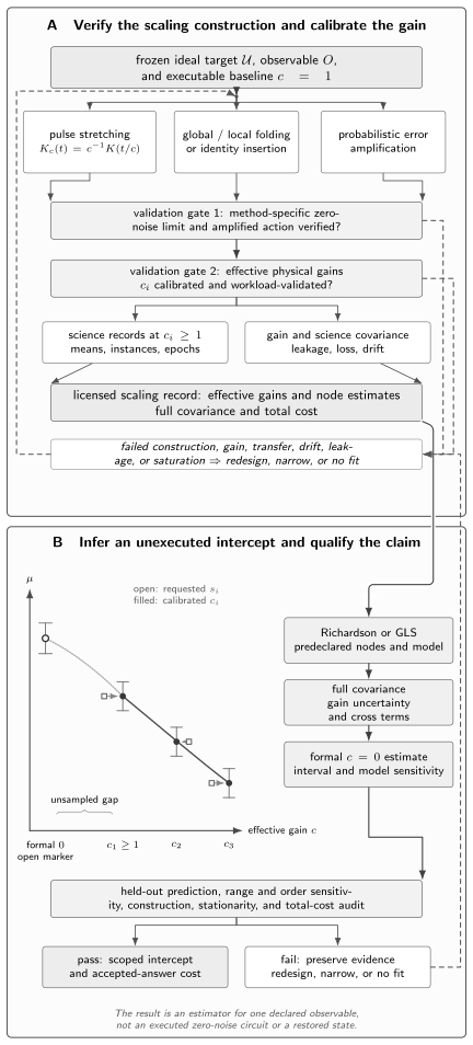
Zero-noise extrapolation audit from method-specific scaling checks through calibrated gains and covariance-aware intercept inference — Zero-noise extrapolation begins with one frozen ideal target, not with a preferred fit. Folding and stretching must preserve the noiseless target, while probabilistic amplification must reduce to it at zero learned noise and realize the declared amplified ensemble at finite gain. Only then do calibrated effective gains and covariance-aware inference support the formal $c=0$ intercept; failed construction, transfer, drift, leakage, or saturation checks require redesign, a narrower claim, or no fit.

Construct an Ideal-Equivalent Noise-Scaling Family

Define a scaled family of channels

The analytic starting point is a local weak-noise expansion

\mu(c;\eta) = \mu_{0|\eta}+ \sum_{k=1}^{p}a_k(c\epsilon)^k +R_{p+1}(c\epsilon).

The coefficients depend on the circuit, observable, state, device context, and chosen scaling path. Smoothness over the fitted range is an assumption to be tested, not a property supplied by the word “noise.” Temme, Bravyi, and Gambetta (2017) gave perturbative constructions that can include more than a strictly Markovian semigroup under suitable rescaling assumptions. Conversely, Schultz et al. (2022) showed why time correlations can make an implementable scaling operation change the sampled spectrum and degrade extrapolation. Non-Markovianity is therefore neither an automatic failure theorem nor a free license: the question is whether this intervention traces a stable, sufficiently smooth family for this target.

The remainder notation should not be overread. A polynomial that describes a neighborhood of $c\epsilon=0$ may cease to be controlled at the largest executable gain. Thresholds, saturation, leakage transitions, coherent oscillations, or a control-regime change can make higher amplification less informative about the intercept. The scaling range is part of the model, and $c_{\max}$ must be justified physically and predictively.

Separate nominal from effective gain

Let $s_i$ be a requested fold, duration, insertion, or amplification factor and $c_i$ the effective physical gain inferred from independent diagnostics. Equality $c_i=s_i$ holds only under a licensed noise model. Gate count may scale by three while the observable-relevant stochastic component scales by less, a coherent component cancels, leakage grows faster, and readout remains nearly unchanged. One scalar can also depend on workload, circuit position, layout, and observable, so a randomized-benchmarking decay from an unmatched proxy does not automatically calibrate the science curve.

If actual gains are $\widetilde c_i=c_i+\delta_i$ , nominal Richardson weights return the canceled linear term as

a_1\epsilon\sum_iw_i\delta_i.

Thus gain error creates bias at the very order the estimator claims to remove. Store gain estimates, uncertainty, calibration circuit class, mapping from diagnostic to science gain, epoch, and any shared data. When a single scalar gain is inadequate, use a declared vector or reject the one-dimensional model rather than hiding the discrepancy inside residuals.

Preserve the ideal operation

Every deterministic fold or stretch must approach the same $\mathcal U$ when physical noise is removed. Check ideal simulation after all compiler passes, algebraic inverse identities in the native representation, conserved quantities, classically tractable instances, mirror or Clifford proxies, and leakage-sensitive invariants. If compiler optimization cancels inserted identities, routing differs across factors, a stretched pulse implements a shifted angle, or an inverse is not the intended physical inverse, the experiment has changed both signal and noise.

PEA needs a different check. Its finite-gain ensemble intentionally realizes an amplified channel and generally is not $\mathcal U$ ; the randomized construction must instead reduce to $\mathcal U$ as learned rates or physical noise vanish and realize the declared $e^{G\mathcal L}$ ensemble at finite gain. Individual sampled circuits need not equal $\mathcal U$ . Both the sampling distribution and the finite-instance approximation require evidence. In local folding, preserving the algebraic product is necessary but does not show that the same coherent and stochastic mechanisms were amplified uniformly.

If only a gate family, error source, layer group, or light-cone region is scaled, the intercept means zero contribution from that selected coordinate with all unscaled background retained. It is not the fully noiseless circuit. State the partial target in the reported result.

Tag context, epoch, and circuit instance

Gain and time are easily confounded. Acquiring all baseline circuits first and the largest gains last makes device drift indistinguishable from a scaling law. Randomize or interleave gains, repeat $c=1$ sentinels throughout acquisition, and block the analysis by an epoch short enough for stationarity to be plausible. Retain fold subsets, twirl seeds, pulse versions, calibrations, layouts, jobs, temperatures or other monitored conditions, and complete attempt counts.

Partial folding and probabilistic amplification add between-instance randomness. Report both within-instance shot variance and the between-instance component; more shots on one fold subset do not replace multiple subsets. Majumdar et al. (2023) emphasize interleaving, partial-fold instances, calibration, and saturation checks in digital ZNE practice.

Derive Richardson Extrapolation at the Intercept

Cancel low-order moments

Choose $p+1$ distinct effective gains $c_i$ and form

\widehat\mu_R = \sum_{i=0}^{p}w_i\widehat\mu(c_i).

To preserve the intercept and cancel the first $p$ terms, require

\sum_iw_i=1, \qquad \sum_iw_i c_i^k=0 \quad(k=1,\ldots,p).

These are interpolation conditions. The linear functional that evaluates a degree- $p$ polynomial at zero has Lagrange weights

w_i = \prod_{j\ne i}\frac{c_j}{c_j-c_i}.

For $c=(1,2,3)$ , the weights are $(3,-3,1)$ . Direct substitution gives the moments

\sum_iw_i c_i^k = (1,0,0,6) \quad\text{for}\quad k=0,1,2,3.

The constant survives, the linear and quadratic terms cancel, and the cubic term does not. The absolute-weight sum is $\Lambda=3+3+1=7$ , already warning that finite fluctuations will be amplified.

Expose the residual bias

Assume the node estimators are unbiased for their finite-gain means and that, at the fixed nodes used, the family has the uniform expansion

\mu(c;\eta) = \mu_{0|\eta} +\sum_{k=1}^{p+1}a_k(c\epsilon)^k +O(\epsilon^{p+2}).

Substitution then gives

\mathbb E[\widehat\mu_R]-\mu_{0|\eta} = a_{p+1}\epsilon^{p+1} \sum_iw_i c_i^{p+1} +O(\epsilon^{p+2}),

when the expansion and remainder are controlled over every used node. Lagrange interpolation further gives

\sum_iw_i c_i^{p+1} = (-1)^p\prod_i c_i.

“Order- $p$ cancellation” therefore names the first canceled terms of a model. It is not a universal unbiasedness theorem. The coefficient multiplying the first omitted term can grow with node placement, and the neglected remainder can dominate at large gain. Mohammadipour and Li (2025) make the polynomial bias, variance, overfitting, and model-mismatch tradeoffs explicit; their bounds remain conditional on their stated regularity and error assumptions.

For two nodes $(1,s)$ , first-order cancellation gives

\widehat\mu_R = \frac{s}{s-1}\widehat\mu(1) - \frac{1}{s-1}\widehat\mu(s), \qquad \Lambda=\frac{s+1}{s-1}.

Increasing $s$ improves this coefficient norm, but often worsens circuit duration, model bias, saturation, and device-regime mismatch. Node choice cannot be optimized from weights alone.

Track signed-weight conditioning

For independent node estimates with equal per-shot variance and optimally allocated total shots, the restricted sampling factor is $\Lambda^2$ . The three-node example gives $49$ . This is not a universal overhead: different node variances, durations, correlations, gain-calibration work, random instances, and validation change the comparison. Krebsbach, Trauzettel, and Calzona (2022) analyze the coupled choice of Richardson coefficients and nodes, illustrating why cancellation order and coefficient growth must be optimized together.

Near-coincident gains make the Vandermonde system ill-conditioned and weights large. Widely separated gains can reduce coefficient amplification but sample a less local curve. Report the weight vector, $\Lambda$ , design-matrix singular values or an equivalent condition measure, and sensitivity to plausible gain errors. A high condition number diagnoses finite sensitivity; it does not prove that a well-conditioned design follows the correct physical path.

Signed weights also change covariance contributions. A perfectly common additive term survives because $\sum_iw_i=1$ ; its off-diagonal terms prevent the artificial $\sum_iw_i^2$ amplification produced by a diagonal-only calculation. Nonuniform shared loadings can cancel or reinforce. Compute the direction from the full matrix.

Freeze order and nodes before the holdout

Polynomial order, gains, fit range, constraints, stopping rule, and excluded records are tuning choices. Select them using theory, pilot data, or a dedicated training split, then freeze them before evaluating final science and held-out validation records. Choosing the order with the most favorable intercept or smallest holdout error and reporting that same holdout as confirmation is validation leakage.

Exact interpolation through $p+1$ points has no residual degrees of freedom. When resources permit, collect additional nodes so residuals, leave-one-node-out predictions, and held-out intermediate gains can challenge the chosen order. Report sensitivity across a small prespecified admissible set rather than treating one curve as uniquely implied by the data.

Allocate Shots and Propagate Full Covariance

Allocate heteroscedastic shots

For a fixed linear estimator with independent node records,

\operatorname{Var}(\widehat\mu_R) = \sum_i\frac{w_i^2\sigma_i^2}{N_i},

where $\sigma_i^2$ is the per-shot variance at node $i$ . For an unweighted raw $\pm1$ record whose mean is $\mu(c_i;\eta)$ , $\sigma_i^2=1-\mu(c_i;\eta)^2$ , so heteroscedasticity is ordinary. A response-corrected, quasiprobability-weighted, conditioned, or otherwise transformed record needs its actual per-record variance and covariance. At fixed total shots $N_{\mathrm{tot}}$ , a Lagrange-multiplier calculation gives

N_i = N_{\mathrm{tot}} \frac{|w_i|\sigma_i}{\sum_j|w_j|\sigma_j}, \qquad \operatorname{Var}_{\min} = \frac{\left(\sum_i|w_i|\sigma_i\right)^2}{N_{\mathrm{tot}}}.

Pilot estimates can guide allocation, but adaptation rules and their data use must be declared. If node $i$ takes time $\tau_i$ per attempt, a fixed execution-time budget $C$ instead yields

N_i\propto\frac{|w_i|\sigma_i}{\sqrt{\tau_i}}, \qquad \operatorname{Var}_{\min} = \frac{\left(\sum_i|w_i|\sigma_i\sqrt{\tau_i}\right)^2}{C}.

This difference matters because folded and stretched nodes can be much slower than the baseline.

Retain shared covariance

For the node vector $\widehat{\boldsymbol\mu}$ with covariance $\Sigma_y$ ,

\operatorname{Var}(\widehat\mu_R) = \mathbf w^{\mathsf T}\Sigma_y\mathbf w.

Independent shot noise contributes diagonal terms. Shared readout calibrations, paired circuit instances, common gain estimates, fold or twirl ensembles, and temporal drift can contribute off-diagonal terms. Retain the identifiers needed to estimate them with a block bootstrap, hierarchical model, or explicit repeated-calibration design. Adding independent error bars in quadrature by default discards the acquisition structure.

A useful analysis separates science-shot, random-instance, calibration, and drift components without assuming independence. A reused calibration can induce substantial covariance even with many science shots. An identical additive drift survives normalized weights; cancellation requires a recorded nonuniform loading or block design that makes it estimable.

Propagate gain-calibration uncertainty

The extrapolated quantity depends on both node estimates and calibrated gains:

h(\mathbf y,\mathbf c) = \mathbf w(\mathbf c)^{\mathsf T}\mathbf y.

A first-order propagation is

\operatorname{Var}(h) \approx h_y^{\mathsf T}\Sigma_yh_y +h_c^{\mathsf T}\Sigma_ch_c +2h_y^{\mathsf T}\Sigma_{yc}h_c,

where $h_y$ and $h_c$ are gradients with respect to estimates and gains. The cross term is necessary when science and gain calibration share records, epochs, or fitted nuisance parameters. Near-coincident gains can make $h_c$ large, so treating the abscissae as exact can severely understate uncertainty.

Prefer independent gain diagnostics when they transfer to the workload. Otherwise use a joint errors-in-variables or hierarchical fit, repeated calibration, or a parametric or block bootstrap that resamples the complete design. Coverage should be tested on known-answer circuits; an interval conditional on a wrong gain map can be narrow and wrong.

Fit Curves Without Turning Flexibility into Evidence

Weighted polynomial regression

With more nodes than coefficients, define $X_{ik}=c_i^k$ , data vector $\mathbf y$ , and full covariance $\Sigma$ . Generalized least squares gives

\widehat{\boldsymbol\beta} = (X^{\mathsf T}\Sigma^{-1}X)^{-1} X^{\mathsf T}\Sigma^{-1}\mathbf y,

provided the declared design is full rank and sufficiently conditioned. The intercept $\widehat\beta_0$ estimates $\mu_{0|\eta}=\mu(0;\eta)$ . “Weighted least squares” is accurate only when the covariance used is diagonal; retaining off-diagonal covariance makes this generalized least squares.

An overdetermined low-order model provides residual degrees of freedom that exact Richardson interpolation lacks. Inspect whitened residuals, leave-one-node-out predictions, and a held-out intermediate gain. Polynomial extrapolation remains a local weak-noise model: adding degree until the training curve is perfect converts flexibility into variance and unstable boundary behavior.

Exponential models need physical licenses

For exact global depolarizing-like decay under a suitable folding model, an observable can have

\mu(c)=a+b p^c=a+b e^{-\gamma c}.

That special structure supplies a reason for an exponential ansatz. Endo, Benjamin, and Li (2018) studied exponential extrapolation alongside linear approaches. With known asymptote $a$ , two distinct gains can identify the remaining ideal parameters under the model. With unknown $a$ , at least three distinct gains are needed to identify $a$ , $b$ , and $\gamma$ , and the desired intercept is $a+b$ .

Pauli-noise modes can motivate

\mu(c)=a+\sum_{r=1}^{R}b_r e^{-\gamma_r c}.

Cai (2021) develops multi-exponential extrapolation and its relation to combined mitigation. Multiple modes can create extrema or zero crossings that a single exponential misses, but close rates, weak components, and saturated data make the parameters poorly identifiable. An extra exponential is not evidence merely because it lowers an in-sample residual.

Predeclare range and model choice

Freeze a small candidate set, gain range, order, asymptote assumptions, constraints, exclusion rules, and comparison criterion. Use predictive residuals at held-out intermediate gains, leave-one-node-out stability, condition measures, and sensitivity across admissible models. Do not select by in-sample $R^2$ or by which intercept lies closest to a hoped-for value.

Residual agreement at $c\ge1$ cannot observe the unsampled interval $0<c<1$ . It must be supplemented by noiseless compiler-equivalence checks, known-answer proxy circuits, calibrated gains, range sensitivity, and held-out workload transfer. If several admissible models fit measured nodes but imply materially different intercepts, model uncertainty dominates and the defensible result may be a wide identified range or no fit.

Never hide clipping or bounded fits

Log-linearizing an exponential requires compatible signs and excludes zeros; it also changes the noise model and can introduce finite-sample bias. A constrained intercept, bounded observable, robust loss, regularizer, or excluded saturated point likewise changes the estimator. Declare each choice before final evaluation and validate its bias and coverage.

An out-of-range extrapolated observable is a diagnostic, not permission to clip. Report the raw extrapolate, instability, and sensitivity. If a predeclared constrained model is used, label it as nonlinear and propagate its sampling law directly, for example by a design-respecting bootstrap or simulation-based coverage study.

Scale Digital Circuits and Analog Controls

Global unitary folding

For an ideal unitary $U$ , global folding replaces

U\longmapsto U(U^\dagger U)^n, \qquad s=2n+1.

The noiseless product remains $U$ , but the nominal depth factor $s$ is not automatically an effective noise gain. Giurgica-Tiron et al. (2020) systematized digital folding and partial local constructions. In practice, first compile the target to the native representation, then insert folds and protect them from optimization. Record how physical inverses are synthesized, because an abstract adjoint may require different pulses, durations, calibrations, or routing.

Folding can fail to amplify coherent error. If the erroneous implementation of the inverse is the exact physical inverse of the erroneous forward gate, then

G_\epsilon G_\epsilon^\dagger G_\epsilon=G_\epsilon.

The inserted pair adds no overrotation. Other coherent structures can oscillate or interfere. Twirling may create a more stable stochastic ensemble, but then its distribution, instances, covariance, and overhead are part of the baseline protocol.

Local and partial folding

Gatewise or layerwise folding applies $G_j\mapsto G_j(G_j^\dagger G_j)^n$ to selected operations. Partial folding uses subsets to realize intermediate nominal scales. “Local” must say whether it means individual gates, layers, circuit regions, or an observable light cone. These choices change where additional error, crosstalk, idle time, and spectator activity enter.

Average over multiple predeclared randomized subsets and retain each seed. Between-subset variation is a real uncertainty component, not shot noise. Pascuzzi et al. (2022) developed computationally efficient identity-insertion constructions; He et al. (2020) studied identity insertions for gate-error mitigation. Both still require compiler protection, matched routing and scheduling, effective-gain calibration, and workload transfer. A finer nominal factor is not necessarily a more nearly scalar physical path.

Pulse stretching

Let a control Hamiltonian $K(t)$ implement the target over $0\le t\le T$ . Define

K_c(t)=\frac{1}{c}K(t/c), \qquad 0\le t\le cT.

Changing variables shows that the ideal unitary is preserved. Under a stationary, control-independent Markovian generator, the longer duration can scale dissipative exposure by $c$ . Kandala et al. (2019) implemented pulse stretching experimentally while recalibrating amplitudes and control corrections.

Real controls require stronger tests. Stretching can alter bandwidth distortion, detuning and Stark shifts, drive-dependent decoherence, idling, heating, crosstalk, leakage, and filter functions. Under colored or time-correlated noise, it can sample a different spectrum rather than multiply one generator. Maupin et al. (2024) found on a particular trapped-ion testbed that time stretching and sideband-detuning scaling did not provide a useful extrapolable family, while global identity insertion performed better but still did not meet the study’s chemical-accuracy target. That is a platform- and protocol-scoped result, not a universal ranking.

Probabilistic error amplification

After an explicitly validated Pauli twirl, model a learned sparse Pauli–Lindblad layer as

\mathcal E=e^{\mathcal L}, \qquad \mathcal L(\rho) = \sum_i\lambda_i(P_i\rho P_i-\rho).

Probabilistic error amplification (PEA) samples an additional physical Pauli channel $e^{(G-1)\mathcal L}$ , giving modeled total noise $e^{G\mathcal L}$ for $G\ge1$ . For one Pauli generator, the inserted error probability is

p_i(G)=\frac{1-e^{-2(G-1)\lambda_i}}{2}.

This physical sampling construction requires $\lambda_i\ge0$ and validated Pauli–Lindblad embeddability; a fitted negative rate does not license the probability above. Kim et al. (2023) used learned layer noise, interleaved calibration, probabilistic amplification, and linear and exponential extrapolation in a large experimental study. The license depends on twirling, model learning, epoch stability, workload transfer, random-instance counts, and model uncertainty. At finite $G$ , the ensemble realizes $e^{G\mathcal L}$ rather than the ideal channel; its zero-rate limit must recover the ideal operation. PEA amplifies a physical channel, whereas probabilistic error cancellation samples a signed formal inverse. Mari, Shammah, and Zeng (2021) connect them without erasing that distinction.

Construction	Ideal-invariance argument	Nominal factor	Effective-gain record	Dominant confounder	Validation evidence	Retained owner boundary
Pulse stretching	Monotone time reparameterization preserves the full time-ordered unitary	Duration ratio	Workload-matched decay or generator proxy with uncertainty	Spectrum, control, heating, leakage	Noiseless waveform check, proxy transfer, sentinels	Control page owns waveform engineering
Global folding	$U(U^\dagger U)^n=U$ ideally	Odd depth factor	Calibrated observable-relevant gain	Coherent cancellation, inverse mismatch	Native inverse audit, mirror proxies, holdout	Circuit model owns ideal composition
Local or partial folding	Selected inverse pairs multiply to identity	Folded-gate or layer fraction	Gain by instance and region	Position, crosstalk, subset variability	Multiple frozen seeds and local invariants	Compiler owner retains placement machinery
Identity insertion	Inserted sequence is ideally identity	Identity repetitions	Matched identity-family gain	Optimization removal, idle imbalance	Post-compile inspection and known-answer tasks	Control owner retains pulse realization
Probabilistic error amplification	Ensemble reduces to $\mathcal U$ at zero rates and realizes $e^{G\mathcal L}$ at finite gain	Requested Lindblad gain $G$	Learned-layer effective gain	Twirl or model transfer and drift	Noise-learning holdout and epoch monitors	PEC owner retains signed inverse sampling
Multivariate or region scaling	Each coordinate preserves the ideal target	Vector of requested factors	Calibrated gain vector and covariance	Dimensional growth and interactions	Rank, cross-term, and region-transfer tests	Application owner retains target workflow
Reject/no-fit control	No licensed invariant is asserted	None	Failed or indistinguishable gain	Any failed gate above	Preserved failure record	Overview owns alternative-method choice

Validate the Scaling License Before Extrapolating

Test ideal invariants and leakage monitors

Validation starts before fitting and is method-specific. For deterministic folds and stretches, run noiseless simulation after the final compiler transformations, test inverse-pair and conservation identities, and use classically tractable or Clifford-like circuits that share native gates, layout, scheduling, and observable light cones. A proxy intended to test ideal-operation preservation must be invariant in the noiseless model. For PEA, test recovery of $\mathcal U$ at zero learned noise and realization of the declared amplified ensemble at finite gain. A noise-sensitive experimental proxy is expected to change with gain and cannot be judged by an ideal-invariance tolerance.

Track leakage, loss, invalid outcomes, timeouts, and acceptance unconditionally as well as conditionally. Folding relies on identities inside the computational subspace; leaked population can escape, return, or be discarded differently as depth grows. If the amplified circuits change yield or sector composition, an accepted conditional expectation and an unconditional contribution are different targets. Neither may silently replace the original ideal observable.

Validate gains on matched workloads

Calibrate effective gains independently on mirror, Clifford, cycle, conservation-law, or classically simulable circuits matched in qubits, depth, native operations, layout, scheduling, and relevant observable support. Average fidelity or one benchmarking decay is insufficient when the science observable responds to different error modes. Device Characterization supplies the broader experimental-design boundary; ZNE owns the transfer from those diagnostics to its scaling coordinate.

Retain gain uncertainty and test monotonic distinguishability over the chosen range. If two requested factors are statistically indistinguishable, the interpolation design is not the nominal Vandermonde system. If one physical mechanism scales and another remains fixed, use a partial-intercept claim or a multivariate model. If gain depends materially on workload class, narrow the domain rather than averaging incompatible coordinates.

Randomize order and block by epoch

Interleave gains and random instances, repeat baseline sentinels, and preserve acquisition timestamps. Analyze residuals against time, batch, layout, fold subset, and calibration epoch. A slope with gain that disappears after time blocking is drift, not a scaling curve. A curve that transfers only within one short epoch may still support a narrow claim if calibration and science records share that stated interval.

Do not reuse an old gain calibration merely because the nominal circuit transformation is unchanged. Define expiry rules from sentinel drift, device recalibration, compiler or pulse version, or failed holdouts. A recalibration policy consumes circuits and wall-clock time and belongs in the resource ledger.

Reject, redesign, or narrow the claim

Acceptance requires a conjunction: method-specific construction checks, effective-gain calibration, local smoothness diagnostics, stationarity, intercept identifiability, complete outcome accounting, and held-out transfer. Failure of one premise cannot be compensated by a visually better regression. For a deterministic fold or stretch, a prespecified known-answer proxy that violates its ideal-invariance tolerance vetoes the family before science extrapolation. PEA instead fails when its zero-rate limit or declared finite-gain ensemble check fails.

Redesign may mean a smaller range, lower order, different folding family, more random instances, another schedule, vector gains, or richer leakage and loss outcomes. Narrow the claim when only one observable class, region, depth, layout, or epoch is licensed. Report no fit when invariance fails, drift aliases gain, saturation leaves the intercept unidentifiable, coherent behavior oscillates, the design is ill-conditioned, or held-out prediction fails. No fit is a scientific output.

Proposed claim	Required license	Raw record	Diagnostic	Falsifier	Response	Residual claim
Ideal-operation invariance	Deterministic maps preserve $\mathcal U$ ; PEA has the declared zero-rate and finite-gain limits	Final native circuits, pulses, or ensemble	Noiseless invariants, ensemble checks, and known-answer proxies	Method-specific construction fails	Redesign or reject	None until restored
Calibrated gain	Requested factor maps to effective $c_i$	Gain diagnostics and uncertainty	Distinguishability and workload transfer	Effective gains unresolved, nontransferable, nonmonotone, or incompatible with the scalar map	Use calibrated nodes, recalibrate, vectorize, narrow, or reject	Partial coordinate only
Smooth local model	One expansion holds over the range	Node estimates and residuals	Held-out and range sensitivity	Oscillation, threshold, or order instability	Shrink range or no fit	Validated local interval
Stationarity	Gain is not aliased with epoch	Timestamps, jobs, sentinels	Time-block and order residuals	Baseline drift explains curve	Reblock or reacquire	One licensed epoch
Intercept identifiability	Design and data constrain $c=0$	Gains, covariance, model set	Rank, condition, model spread	Saturation or divergent admissible intercepts	Lower order or no fit	Identified set if useful
Complete outcome accounting	Leakage, loss, failure, and acceptance retained	Attempt-level outcome space	Yield and sector audit	Scale-dependent hidden rejection	Enlarge target record	Explicit conditional target
Workload transfer	Proxies represent the science response	Matched held-out circuits	Predictive coverage and residuals	Proxy success does not transfer	Narrow or reject	Named workload class

Audit Bias, Variance, and Total Cost Together

Compute signed-sampling overhead

Bias cancellation and variance amplification must be reported together. For a chosen model and gain range, calculate the first uncanceled moment or a justified remainder bound, the full covariance, gain uncertainty, and sensitivity across admissible models. The coefficient norm $\Lambda$ is a useful early warning, but it omits circuit duration, random-instance variation, calibration, validation, failures, and model bias. A higher cancellation order can be worse at fixed total cost even when its asymptotic power of $\epsilon$ is better.

Multivariate scaling makes this tension explicit. For independently scalable coordinates $\boldsymbol\lambda$ ,

\mu(\boldsymbol\lambda) = \mu_{0|\eta}+ \sum_{1\le|\boldsymbol\alpha|\le d} a_{\boldsymbol\alpha}\boldsymbol\lambda^{\boldsymbol\alpha} +R_{d+1}(\boldsymbol\lambda),

and a linear estimator cancels selected monomials through

\sum_iw_i=1, \qquad \sum_iw_i\boldsymbol\lambda_i^{\boldsymbol\alpha}=0.

Otten and Gray (2019) varied distinct relaxation-like properties to recover observables. Layerwise Richardson treats layers or coarse circuit regions as coordinates; Russo and Mari (2024) develop this construction using multivariate interpolation. With $\ell$ coordinates and total degree $d$ , a full design requires at least

M=\binom{d+\ell}{d}

nodes before replication. Circuit count, gain calibration, cross terms, and coefficient norms therefore grow quickly. Physics-informed regions or observable light cones are usually more defensible than one coordinate per gate.

Include every resource ledger

“No extra qubits” does not mean “no quantum overhead.” Count baseline and amplified science attempts, accepted and rejected outcomes, fold or twirl instances, deeper gates or pulse duration, calibration and noise-learning circuits, repeated sentinels, held-out validation, queue and wall-clock time, compiler work, classical inference, and failed scaling families. Separate quantities that are directly counted from those projected under stationarity or amortization.

The ledger also names reused artifacts. A shared response calibration induces covariance, a learned Pauli model has an expiry interval, and a compiler-equivalence audit belongs to one version. For amortized costs, state the number and class of science tasks. Untested reuse is not free evidence.

Ledger item	Primitive record	Transformation	Uncertainty	Diagnostic	Resource unit	Claim boundary
Estimand and raw baseline	Target, $c=1$ attempts and outcomes	Raw mean and acceptance	Shot and epoch variation	Repeated sentinels	Attempts and time	Named observable and context
Circuit and compiler	Native circuit, layout, versions	Fold or stretch insertion	Instance and version effects	Noiseless equivalence	Gates, depth, duration	Same ideal target only
Scaling construction	Requested factors and instances	Physical amplification map	Between-instance variation	Invariance monitor	Circuits and random seeds	Licensed construction
Gain calibration	Matched diagnostic records	Nominal-to-effective map	Gain and cross covariance	Workload transfer	Calibration attempts	Named gain coordinate
Science acquisition	Outcomes by gain, time, and job	Node estimates	Heteroscedastic shot noise	Time and instance residuals	Science attempts	Frozen acquisition design
Covariance and resampling	Batch and shared-record identifiers	GLS, bootstrap, or hierarchy	Full matrix and coverage	Known-answer coverage	Classical compute and storage	Declared dependence model
Model and fit	Frozen nodes, order, constraints	Richardson or regression	Remainder and model spread	Condition and leave-one-out	Fit time and candidate count	Prespecified candidate set
Held-out validation and failures	Proxy and rejected-family records	Predictive comparison	Transfer uncertainty	Invariance, gain, drift, saturation	Validation attempts	Accept, narrow, redesign, or no fit
Total resources	All attempted work and reuse policy	Matched-budget aggregation	Amortization sensitivity	Cost-to-accepted-answer	Shots, circuits, time, qubits, compute	Finite scoped quality–cost claim

Match accepted-answer budgets

Compare unmitigated and mitigated procedures under honest budgets such as equal raw science shots, total attempts, and wall-clock time. For a fixed standard error or accuracy probability, report projected and observed cost to an accepted answer, including failed jobs and postselection.

A ZNE estimate can reduce observed bias while increasing mean-squared error because signed variance dominates. Conversely, a more expensive procedure can be worthwhile for a prespecified finite task. The conclusion must name the task, error metric, validation set, and budget. Do not generalize one finite advantage to scalable computation, and do not use an asymptotic lower bound to erase a demonstrated finite result outside the bound’s assumptions.

Compose ZNE with Other Interventions Carefully

Account for measurement response in the full estimator

Folding and pulse stretching normally do not scale terminal response error. Because $\sum_iw_i=1$ , a scale-independent additive response bias survives Richardson combination. Account for terminal response in the complete estimator and propagate shared calibration covariance across nodes. Do not calibrate readout at only the baseline and assume transfer to longer, leakier, or temporally separated circuits.

For a fixed scale-independent affine response transform $T(\mathbf q)=L\mathbf q+\mathbf b$ and fixed linear ZNE weights, algebra gives

\sum_iw_iT(\widehat{\mathbf q}_i) = T\!\left(\sum_iw_i\widehat{\mathbf q}_i\right),

because $\sum_iw_i=1$ . Thus correction may be applied per node or after combination only when scale independence, affine equivalence, and the full shared-calibration covariance are demonstrated. Response drift, gain-dependent calibrations, regularization, clipping, simplex projection, constraints, or other nonlinear operations destroy that equivalence and require a per-node or joint treatment. The measurement specialist owns the response license; the ZNE analysis owns how its uncertainty and reuse enter the node covariance.

Conditioning makes composition order-dependent

For a compatible jointly measurable observable, normally $[O,\Pi]=0$ , symmetry verification can estimate the conditional ratio

\langle O\rangle_{\mathrm{sym}} = \frac{\langle O\Pi\rangle}{\langle\Pi\rangle}.

Without that compatibility, use the Lüders-projected expression $\langle\Pi O\Pi\rangle/\langle\Pi\rangle$ and retain its covariance. One can extrapolate numerator and denominator jointly with their covariance, or extrapolate the already conditioned ratio at each gain. These are different nonlinear estimators and need not agree. Freeze the choice, retain rejected attempts and acceptance by gain, and validate the complete composition. A denominator approaching zero under amplification can make an otherwise smooth numerator useless.

The same rule applies to constrained readout correction, robust regression, adaptive node selection, and optimizer feedback. Component-level validation does not establish that the ordered stack preserves the target, covariance, or coverage. Tuning any component on the final holdout makes that holdout part of training.

Keep suppression, cancellation, and correction owners distinct

Randomized compiling or twirling can make coherent behavior more reproducible in some regimes, but then it is part of the frozen baseline and its random ensemble is costed. Dynamical decoupling suppresses or filters physical noise; if combined with stretching or folding, hold its schedule fixed and revalidate the filter function. PEA amplifies a learned channel, whereas probabilistic error cancellation uses signed quasiprobability sampling to approximate an inverse. These methods can share models without becoming interchangeable.

VQE retains optimizer placement, objective estimation, measurement allocation, and data-reuse decisions. Digital Quantum Simulation retains mapping, synthesis, and product-formula error budgets. A joint extrapolation in physical-noise strength and Trotter step is a developing multivariate method, not ordinary one-coordinate ZNE. Noise Simulation can generate diagnostics and synthetic coverage studies but cannot replace device transfer evidence. Encoded correction and logical protection require the QEC owners.

Recognize Regimes Where ZNE Fails

Coherent errors can cancel or oscillate

Inverse pairs can cancel a coherent overrotation, amplify a different coherent component, or generate oscillations with fold count. A monotone decay model can then return a stable-looking but wrong intercept. Inspect signed residuals, multiple intermediate gains, randomized instances, and a model capable of falsifying monotonicity. Twirling may help for a declared ensemble, but it changes the protocol and does not guarantee a scalar path.

Control asymmetry matters: the physical implementation of $G^\dagger$ may have different duration, calibration, crosstalk, or leakage from $G$ . An identity sequence that is exact in algebra can introduce a structured signal error after compilation. Reject target invariance before interpreting the curve as noise scaling.

Memory, crosstalk, leakage, and loss can break scalar scaling

Pulse stretching changes the time available for environmental memory and the frequencies sampled by the control filter. Local folds change spectator schedules and the spatial pattern of crosstalk. Leakage makes $G^\dagger G=I$ false outside the computational subspace, and scale-dependent loss or timeouts can silently condition the sample. These effects may demand a vector gain, a richer outcome space, a narrower claim, or no fit.

The Markovian and Non-Markovian Noise page owns the correlation-regime theory. The ZNE question is operational: does the chosen amplification and workload admit a stable path with predictive held-out behavior? Global scaling can sometimes remain useful when a local rule fails, and some perturbative non-Markovian models remain expandable. Avoid both “memory always defeats ZNE” and “smooth training data prove memory is harmless.”

Saturation can destroy intercept information

At strong noise, observables can approach an asymptote nearly independent of the ideal target. Several saturated nodes may have tiny residuals under many models while containing little information about $c=0$ . Diagnose design rank, profile or bootstrap intercept spread, model sensitivity, and whether held-out tasks with different ideal answers remain distinguishable. More shots on a flat saturated curve improve precision around the wrong part of the path, not identifiability of the intercept.

Takagi et al. (2022) prove severe sampling limitations for specified broad mitigation and noise settings. Keep those assumptions and accuracy criteria attached to the claim; the result is not “all finite ZNE is useless.” Separately, high-order Richardson coefficients can grow rapidly for common node choices. A practical no-fit decision can arise well before an asymptotic theorem applies, from finite conditioning, saturation, drift, or failed transfer.

Three Reproducible ZNE Audits

Audit 1 — Richardson cancellation and cubic remainder

Take effective gains $(1,2,3)$ and derive the weights rather than entering them as a fit result. The interpolation system returns $(3,-3,1)$ , cancels the linear and quadratic moments, and leaves cubic moment $6$ . For

\mu(c) = 0.42-0.30(c\epsilon) +0.18(c\epsilon)^2 -0.07(c\epsilon)^3, \qquad \epsilon=0.04,

the node values are $0.40828352$ , $0.39711615999999994$ , and $0.38647104$ . Their Richardson combination is $0.4199731200000003$ , with cubic bias $-0.00002688$ . This equality belongs to the finite cubic fixture. It is not a bound for an unknown experimental remainder. The factor $49=\Lambda^2$ is likewise the restricted homoscedastic, independent, optimally allocated total-shot factor—not a universal protocol overhead.

Audit 2 — Covariance and optimal allocation

Keep the same weights, per-shot standard deviations $(0.6,0.8,0.5)$ , and total budget $47000$ . Independent-shot optimal allocation is $(18000,24000,5000)$ , giving node variances $0.00002$ , $0.0000266666666667$ , and $0.00005$ , and estimator variance $0.00047$ . The independently sampled shot component is diagonal.

Now add a common additive covariance $\tau^2=0.000002$ to every matrix entry. The diagonal-only calculation becomes $0.000508$ , while the full form is $0.000472$ with standard error $0.021725560982400433$ . Because $\sum_iw_i=1$ , the common contribution survives as $\tau^2$ ; negative cross terms remove only the spurious $\tau^2\sum_iw_i^2$ amplification from diagonal-only accounting. Other covariance patterns can increase or decrease uncertainty. Continuous equal allocation gives independent variance $0.0005904255319148936$ .

Audit 3 — Effective-gain calibration and rejection

Suppose nominal gains $(1,2,3)$ are actually $(1,1.8,2.55)$ . Evaluating the same cubic curve and reconstructing the weights at those effective gains gives

\begin{aligned} \boldsymbol\mu_{\rm eff} &= \begin{pmatrix} 0.40828352\\ 0.39930699264\\ 0.39119843544 \end{pmatrix},\\ \boldsymbol\gamma_{\rm eff} &\approx \begin{pmatrix} 3.701612903225807\\ -4.25\\ 1.5483870967741944 \end{pmatrix}. \end{aligned}

Nominal weights return $0.41812801752$ , bias $-0.00187198248$ . The calibrated weights give estimate $0.4199794368$ , but raise $\Lambda$ from $7$ to $9.5$ and its restricted square from $49$ to $90.25$ .

The gain correction is not the final gate. Treat $(1,0.997,0.989)$ as values of a noiseless simulator/compiler-equivalence proxy that should stay at one, with predeclared tolerance $0.005$ . Its scale-three deviation $0.011$ fails. The scaling family is rejected before extrapolation even though the calibrated weights improve this polynomial fixture. A noise-sensitive experimental proxy expected to decay with gain would not be a valid invariant for this test.

const tolerance = 1e-12;

function assertClose(actual, expected, label) {
  if (!Number.isFinite(actual) || Math.abs(actual - expected) > tolerance) {
    throw new Error(`${label}: expected ${expected}, received ${actual}`);
  }
}

function assertArrayClose(actual, expected, label) {
  if (actual.length !== expected.length) {
    throw new Error(`${label}: length mismatch`);
  }
  actual.forEach((value, position) => {
    assertClose(value, expected[position], `${label}[${position}]`);
  });
}

function richardsonWeights(gains) {
  return gains.map((gain, position) =>
    gains.reduce(
      (product, otherGain, otherPosition) =>
        position === otherPosition
          ? product
          : product * otherGain / (otherGain - gain),
      1,
    ),
  );
}

function dot(left, right) {
  return left.reduce((sum, value, position) => sum + value * right[position], 0);
}

function quadraticForm(vector, matrix) {
  return vector.reduce(
    (outerSum, leftValue, row) =>
      outerSum + leftValue * matrix[row].reduce(
        (innerSum, matrixValue, column) =>
          innerSum + matrixValue * vector[column],
        0,
      ),
    0,
  );
}

const gains = [1, 2, 3];
const weights = richardsonWeights(gains);
assertArrayClose(weights, [3, -3, 1], 'Richardson weights');

const moments = [0, 1, 2, 3].map((power) =>
  dot(weights, gains.map((gain) => gain ** power)),
);
assertArrayClose(moments, [1, 0, 0, 6], 'Richardson moments');

const mu0 = 0.42;
const linearCoefficient = -0.30;
const quadraticCoefficient = 0.18;
const cubicCoefficient = -0.07;
const epsilon = 0.04;
const curve = (gain) =>
  mu0
  + linearCoefficient * gain * epsilon
  + quadraticCoefficient * (gain * epsilon) ** 2
  + cubicCoefficient * (gain * epsilon) ** 3;

const nodeValues = gains.map(curve);
assertArrayClose(
  nodeValues,
  [0.40828352, 0.39711615999999994, 0.38647104],
  'Audit 1 node values',
);
const auditOneEstimate = dot(weights, nodeValues);
const cubicBias = cubicCoefficient * epsilon ** 3 * moments[3];
const absoluteWeightSum = weights.reduce((sum, weight) => sum + Math.abs(weight), 0);
assertClose(auditOneEstimate, 0.4199731200000003, 'Audit 1 estimate');
assertClose(cubicBias, -0.00002688, 'Audit 1 cubic bias');
assertClose(auditOneEstimate - mu0, cubicBias, 'Audit 1 direct bias');
assertClose(absoluteWeightSum, 7, 'Audit 1 absolute-weight sum');
assertClose(absoluteWeightSum ** 2, 49, 'Audit 1 restricted factor');

const perShotStandardDeviations = [0.6, 0.8, 0.5];
const totalShots = 47000;
const allocationNormalizer = dot(
  weights.map(Math.abs),
  perShotStandardDeviations,
);
const optimalAllocation = weights.map((weight, position) =>
  totalShots * Math.abs(weight) * perShotStandardDeviations[position]
  / allocationNormalizer,
);
assertArrayClose(optimalAllocation, [18000, 24000, 5000], 'Optimal allocation');

const independentNodeVariances = perShotStandardDeviations.map(
  (standardDeviation, position) =>
    standardDeviation ** 2 / optimalAllocation[position],
);
assertArrayClose(
  independentNodeVariances,
  [0.00002, 0.0000266666666667, 0.00005],
  'Independent node variances',
);
const independentVariance = dot(
  weights.map((weight) => weight ** 2),
  independentNodeVariances,
);
assertClose(independentVariance, 0.00047, 'Independent estimator variance');

const commonVariance = 0.000002;
const fullCovariance = independentNodeVariances.map((variance, row) =>
  independentNodeVariances.map((unused, column) =>
    commonVariance + (row === column ? variance : 0),
  ),
);
assertArrayClose(
  fullCovariance.map((row, position) => row[position]),
  [0.000022, 0.0000286666666667, 0.000052],
  'Full covariance diagonal',
);
fullCovariance.forEach((row, rowPosition) => {
  row.forEach((value, columnPosition) => {
    if (rowPosition !== columnPosition) {
      assertClose(value, 0.000002, 'Full covariance off diagonal');
    }
  });
});
const diagonalOnlyVariance = dot(
  weights.map((weight) => weight ** 2),
  fullCovariance.map((row, position) => row[position]),
);
const fullVariance = quadraticForm(weights, fullCovariance);
assertClose(diagonalOnlyVariance, 0.000508, 'Diagonal-only variance');
assertClose(fullVariance, 0.000472, 'Full-covariance variance');
assertClose(Math.sqrt(fullVariance), 0.021725560982400433, 'Full standard error');

const equalAllocation = totalShots / gains.length;
const equalAllocationVariance = weights.reduce(
  (sum, weight, position) =>
    sum + weight ** 2 * perShotStandardDeviations[position] ** 2 / equalAllocation,
  0,
);
assertClose(
  equalAllocationVariance,
  0.0005904255319148936,
  'Continuous equal-allocation variance',
);

const effectiveGains = [1, 1.8, 2.55];
const effectiveNodeValues = effectiveGains.map(curve);
assertArrayClose(
  effectiveNodeValues,
  [0.40828352, 0.39930699264, 0.39119843544],
  'Audit 3 node values',
);
const nominalEstimate = dot(weights, effectiveNodeValues);
assertClose(nominalEstimate, 0.41812801752, 'Nominal-gain estimate');
assertClose(nominalEstimate - mu0, -0.00187198248, 'Nominal-gain bias');

const effectiveWeights = richardsonWeights(effectiveGains);
assertArrayClose(
  effectiveWeights,
  [3.701612903225807, -4.25, 1.5483870967741944],
  'Effective-gain weights',
);
const effectiveWeightSum = effectiveWeights.reduce(
  (sum, weight) => sum + Math.abs(weight),
  0,
);
const effectiveEstimate = dot(effectiveWeights, effectiveNodeValues);
assertClose(effectiveWeightSum, 9.5, 'Effective absolute-weight sum');
assertClose(effectiveWeightSum ** 2, 90.25, 'Effective restricted factor');
assertClose(effectiveEstimate, 0.4199794368, 'Effective-gain estimate');
assertClose(effectiveEstimate - mu0, -0.0000205632, 'Effective-gain cubic bias');

const idealInvariantProxies = [1, 0.997, 0.989];
const invarianceTolerance = 0.005;
const scaleThreeDeviation = Math.abs(
  idealInvariantProxies[2] - idealInvariantProxies[0],
);
assertClose(scaleThreeDeviation, 0.011, 'Scale-three invariant deviation');
if (!(scaleThreeDeviation > invarianceTolerance)) {
  throw new Error('The scaling family should be rejected');
}

console.log('Zero-noise-extrapolation finite audits: PASS');

Canonical Owners and Common Claim Failures

Canonical handoffs

Use the chapter guide for the discrepancy-to-model workflow and the Error Mitigation Overview for the cross-family decision among suppression, response correction, extrapolation, cancellation, filtering, encoded correction, or no intervention. This page begins after those declarations and retains only the physical scaling and intercept-inference problem.

Use Control, Readout, and Calibration for pulse, inverse-gate, readout, feedback, and recalibration engineering; Device Characterization for diagnostic experimental design; and Reporting Standards for durable raw-data, provenance, versioning, and executable-record requirements. The application pages retain algorithm-specific interpretation and resource budgets. Formal mitigation limitations remain with Lower Bounds and Limitations.

Probabilistic Error Cancellation owns inverse-channel quasiprobability sampling; Symmetry Verification owns sector conditioning, projection, check calibration, and acceptance accounting; Dynamical Decoupling owns filter functions and pulse sequences; and QEC pages own encoded recovery and logical protection. Cross-link rather than importing those derivations into a ZNE fit. This page retains physical scaling, effective-gain calibration, covariance, intercept inference, and no-fit decisions.

Common claim failures

Nominal scale is called physical gain. Report requested and calibrated factors separately with their diagnostic, transfer domain, uncertainty, and epoch.

A fit validates the family that produced it. Use independent construction, gain, stationarity, outcome, and workload-transfer tests. Residuals do not establish the physical family.

Higher Richardson order is called automatically better. Compare the first omitted term, coefficient norm, covariance, gain sensitivity, circuit cost, and held-out prediction at the same total budget.

A diagonal error bar hides shared records. Reconstruct $\mathbf w^{\mathsf T}\Sigma\mathbf w$ from the acquisition design and propagate gain, calibration, instance, and drift components with their cross terms.

Saturated points are praised for their small scatter. Ask whether different known ideal answers remain distinguishable. Precision near a noise asymptote is not information about the zero-noise intercept.

Unphysical-looking extrapolates are clipped. Preserve them as instability evidence. A predeclared constrained estimator is a new nonlinear procedure with its own bias and coverage.

Loss or leakage disappears from the denominator. Report attempts, accepted records, conditional expectations, and unconditioned contributions separately, with scale-dependent yield and covariance.

Validated components are treated as a validated stack. Freeze the operation order, then test the complete procedure on held-out tasks.

A finite improvement is called state restoration or fault tolerance. ZNE estimates a declared expectation from an ensemble. It does not repair a state, correct one trajectory, or protect encoded quantum information.

One failure or lower bound is made universal. Keep device failures, finite successes, and theorems inside their scaling construction, workload, noise class, accuracy criterion, and resource model.

Exercises

1. Derive Richardson weights and the first uncanceled moment. For gains $(1,2,4)$ , derive the quadratic Richardson weights, their absolute-weight sum, and the cubic moment. Explain what the sign and magnitude of that moment do and do not establish.

Solution

The interpolation formula gives $w=(8/3,-2,1/3)$ . The zeroth moment is one and the first two moments vanish. The absolute-weight sum is $5$ . The cubic moment is $8/3-16+64/3=8$ , agreeing with $c_0c_1c_2$ for $p=2$ . Thus the leading cubic contribution is $8a_3\epsilon^3$ when the local expansion is controlled; it is not a bound on an unknown remainder or model mismatch.

2. Optimize a heteroscedastic shot allocation. A two-node estimator has weights $(2,-1)$ , per-shot standard deviations $(0.5,1)$ , and $12000$ total independent shots. Find the continuous optimal allocation and variance. Compare with equal allocation.

Solution

The allocation factors are $(|2|0.5,|-1|1)=(1,1)$ , so both nodes receive $6000$ shots. The variance is $4(0.25)/6000+1/6000=1/3000$ . Equal allocation happens to be optimal because the absolute-weighted standard deviations match. Equal shots would not generally be optimal merely because there are two nodes.

3. Propagate correlated node uncertainty. Recompute Audit 2’s common-mode contribution directly from $\tau^2\mathbf1\mathbf1^{\mathsf T}$ . Why is it much smaller than the same component in a diagonal-only calculation?

Solution

The full contribution is $\tau^2(\mathbf1^{\mathsf T}\mathbf w)^2=0.000002$ . Keeping only its diagonal gives $\tau^2\sum_iw_i^2=0.000038$ . The identical additive mode survives because the weights sum to one; cross terms remove only the artificial signed-weight amplification. Another loading can reinforce or partly cancel, so retain the full matrix.

4. Audit effective-gain miscalibration. Nominal gains $(1,2,3)$ use weights $(3,-3,1)$ , but actual gains are $(1,1.9,3.2)$ . Calculate the returned linear moment and state the leading bias it creates.

Solution

The actual linear moment is $3(1)-3(1.9)+3.2=0.5$ . A curve with linear coefficient $a_1$ and baseline strength $\epsilon$ therefore retains leading term $0.5a_1\epsilon$ . More science shots do not remove this systematic gain error. One must calibrate gains and recompute weights with uncertainty, adopt a richer model, or reject the scalar family.

5. Compare folding and pulse stretching licenses. Give two ideal-operation checks and three physical-scaling falsifiers for each construction. Explain why neither nominal factor alone identifies the gain.

Solution

For folding, check the final native noiseless product and the synthesized inverse pairs; falsifiers include compiler removal, coherent cancellation or oscillation, and changed routing or crosstalk. For stretching, check the rescaled noiseless unitary and calibrated rotation angle; falsifiers include bandwidth distortion, drive-dependent decoherence, and changed leakage or noise spectrum. Depth and duration describe interventions, but the observable-relevant physical mechanisms can scale differently.

6. Diagnose a saturated no-fit regime. Four high-gain points have tiny standard errors and nearly equal means. List four analyses needed before extrapolating and give a defensible decision if matched known-answer circuits with different ideals also collapse to that mean.

Solution

Inspect design and profile-intercept conditioning, model and range sensitivity, held-out intermediate-gain residuals, and distinguishability on matched known-answer tasks; also examine time and leakage records. If distinct ideal targets collapse to one high-noise asymptote, those nodes contain little intercept information. More shots improve precision at the asymptote. The defensible result is no fit or a redesigned smaller-gain experiment, not a narrow extrapolated interval.

7. Design a multivariate scaling audit. For three independently scalable circuit regions and total polynomial degree two, find the minimum full design size before replication. What must an intercept mean if only two regions are scaled?

Solution

$M=\binom{2+3}{2}=10$ nodes are required for all monomials through total degree two before repeated shots, random instances, calibration, and validation. The design must test rank, interactions, gain covariance, target invariance, and coefficient norm. If only two regions are scaled, the intercept removes the modeled contributions of those coordinates while retaining the third region and all other unscaled errors; it is not the fully noiseless circuit.

8. Scope a composed mitigation claim. A team applies readout correction, symmetry conditioning, and ZNE. Specify a defensible order and uncertainty analysis, and list the evidence needed before claiming improvement.

Solution

One defensible design corrects the joint numerator and denominator records at every gain, extrapolates them jointly with response, node, gain, and cross covariance, then forms the predeclared ratio. Another extrapolates conditioned ratios, but it is a different nonlinear estimator. Retain rejected attempts and scale-dependent acceptance. Freeze all tuning, validate the complete order on matched held-out tasks, compare at total attempted and wall-clock budgets, and report only an improved expectation estimate—not a restored state or logical protection.

References

Z. Cai, “Multi-Exponential Error Extrapolation and Combining Error Mitigation Techniques for NISQ Applications,” npj Quantum Information 7, 80 (2021), doi:10.1038/s41534-021-00404-3.
S. Endo, S. C. Benjamin, and Y. Li, “Practical Quantum Error Mitigation for Near-Future Applications,” Physical Review X 8, 031027 (2018), doi:10.1103/PhysRevX.8.031027.
T. Giurgica-Tiron, Y. Hindy, R. LaRose, A. Mari, and W. J. Zeng, “Digital Zero Noise Extrapolation for Quantum Error Mitigation,” in 2020 IEEE International Conference on Quantum Computing and Engineering (QCE), 306–316 (IEEE, 2020), doi:10.1109/QCE49297.2020.00045.
A. He, B. Nachman, W. A. de Jong, and C. W. Bauer, “Zero-Noise Extrapolation for Quantum-Gate Error Mitigation with Identity Insertions,” Physical Review A 102, 012426 (2020), doi:10.1103/PhysRevA.102.012426.
A. Kandala, K. Temme, A. D. Córcoles, A. Mezzacapo, J. M. Chow, and J. M. Gambetta, “Error Mitigation Extends the Computational Reach of a Noisy Quantum Processor,” Nature 567, 491–495 (2019), doi:10.1038/s41586-019-1040-7.
Y. Kim, A. Eddins, S. Anand, K. X. Wei, E. van den Berg, S. Rosenblatt, H. Nayfeh, Y. Wu, M. Zaletel, K. Temme, and A. Kandala, “Evidence for the Utility of Quantum Computing before Fault Tolerance,” Nature 618, 500–505 (2023), doi:10.1038/s41586-023-06096-3.
M. Krebsbach, B. Trauzettel, and A. Calzona, “Optimization of Richardson Extrapolation for Quantum Error Mitigation,” Physical Review A 106, 062436 (2022), doi:10.1103/PhysRevA.106.062436.
Y. Li and S. C. Benjamin, “Efficient Variational Quantum Simulator Incorporating Active Error Minimization,” Physical Review X 7, 021050 (2017), doi:10.1103/PhysRevX.7.021050.
R. Majumdar, P. Rivero, F. Metz, A. Hasan, and D. S. Wang, “Best Practices for Quantum Error Mitigation with Digital Zero-Noise Extrapolation,” in 2023 IEEE International Conference on Quantum Computing and Engineering (QCE), vol. 1, 881–887 (IEEE, 2023), doi:10.1109/QCE57702.2023.00102.
A. Mari, N. Shammah, and W. J. Zeng, “Extending Quantum Probabilistic Error Cancellation by Noise Scaling,” Physical Review A 104, 052607 (2021), doi:10.1103/PhysRevA.104.052607.
O. G. Maupin, A. D. Burch, B. Ruzic, C. G. Yale, A. Russo, D. S. Lobser, M. C. Revelle, M. N. Chow, S. M. Clark, A. J. Landahl, and P. J. Love, “Error Mitigation, Optimization, and Extrapolation on a Trapped-Ion Testbed,” Physical Review A 110, 032416 (2024), doi:10.1103/PhysRevA.110.032416.
P. Mohammadipour and X. Li, “Direct Analysis of Zero-Noise Extrapolation: Polynomial Methods, Error Bounds, and Simultaneous Physical-Algorithmic Error Mitigation,” Quantum 9, 1909 (2025), doi:10.22331/q-2025-11-14-1909.
M. Otten and S. K. Gray, “Recovering Noise-Free Quantum Observables,” Physical Review A 99, 012338 (2019), doi:10.1103/PhysRevA.99.012338.
V. R. Pascuzzi, A. He, C. W. Bauer, W. A. de Jong, and B. Nachman, “Computationally Efficient Zero-Noise Extrapolation for Quantum-Gate-Error Mitigation,” Physical Review A 105, 042406 (2022), doi:10.1103/PhysRevA.105.042406.
V. Russo and A. Mari, “Quantum Error Mitigation by Layerwise Richardson Extrapolation,” Physical Review A 110, 062420 (2024), doi:10.1103/PhysRevA.110.062420.
K. Schultz, R. LaRose, A. Mari, G. Quiroz, N. Shammah, B. D. Clader, and W. J. Zeng, “Impact of Time-Correlated Noise on Zero-Noise Extrapolation,” Physical Review A 106, 052406 (2022), doi:10.1103/PhysRevA.106.052406.
R. Takagi, S. Endo, S. Minagawa, and M. Gu, “Fundamental Limits of Quantum Error Mitigation,” npj Quantum Information 8, 114 (2022), doi:10.1038/s41534-022-00618-z.
K. Temme, S. Bravyi, and J. M. Gambetta, “Error Mitigation for Short-Depth Quantum Circuits,” Physical Review Letters 119, 180509 (2017), doi:10.1103/PhysRevLett.119.180509.