Stabilizer Formalism

Scope

The stabilizer formalism describes an important exact subtheory of qubit quantum mechanics using commuting Pauli constraints instead of generic state amplitudes. The same algebra organizes:

• stabilizer states such as computational-basis, Bell, GHZ, graph, and cluster states;
• stabilizer codes and their logical Pauli operators;
• error syndromes and degeneracy;
• Clifford gates and Pauli propagation;
• efficient classical simulation by binary tableaus.

Pauli Group and Stabilizers is the direct small-list readiness bridge for phase-aware products, generator consistency, stabilized dimension, and algebraic error signatures; this page remains the canonical home of the general Pauli-group and stabilizer formalism. Stabilizer States Preview owns the multipartite-state motivation and worked Bell, GHZ, and graph-state examples. Universal Gate Sets owns Clifford+$T$, synthesis, and universality. Syndrome Measurement owns signed physical check circuits, ordered fault propagation, repeated outcomes, and detector records; this page retains stabilizer projectors, normalizers, syndrome algebra, and the ideal Pauli-measurement update. Three-Qubit Codes owns the concrete repetition-code codewords, logical representatives, syndrome table, ideal lookup recovery, and single-axis protection limits; this page retains the general stabilizer and normalizer algebra. Five-Qubit Code owns the declared cyclic generators, code projector, logical basis, complete one-qubit syndrome lookup, and code-specific full-Pauli distance proof; this page retains the general stabilizer and normalizer algebra. Shor Code owns the eight declared generators, projector, logical representatives, twenty-two one-error syndrome classes, degeneracy, and code-specific distance proof; this page retains general Pauli, symplectic, normalizer, Clifford, and tableau algebra. Steane Code owns the six declared generators, projector, logical representatives, twenty-two occupied one-error syndromes, weak self-duality, and code-specific distance proof; this page retains general Pauli, symplectic, normalizer, Clifford, and tableau algebra. CSS Codes owns paired CSS check matrices, nested-code and coset bases, logical quotients, axis distances, and the CSS correctability specialization; this page retains general Pauli, symplectic, projector, normalizer, Clifford, and tableau theory. Measurement-Based Quantum Computation owns the use of graph stabilizers, Pauli byproducts, adaptive non-Pauli measurements, and flow or gflow in a measurement-pattern model; this page retains the general Pauli, Clifford, and tableau algebra. Decoders owns probabilistic inference among logical equivalence classes; code pages own their syndrome circuits, thresholds, and hardware overhead. Fault-Tolerant Gates owns gadget-level correctness, controlled propagation, and protected logical operation mechanisms.

The central dictionary is:

Quantum object	Stabilizer description
Pauli string	binary phase-space vector plus a phase
commutation	binary symplectic inner product
stabilizer state	unique common $+1$ eigenspace of $n$ independent checks
$[[n,k]]$ stabilizer code	common $+1$ eigenspace of $n-k$ independent checks
syndrome	commutation pattern between an error and the checks
logical Pauli	Pauli preserving the code but not acting trivially on it
Clifford gate	unitary mapping Pauli strings to Pauli strings by conjugation
stabilizer simulation	update generators or a tableau instead of $2^n$ amplitudes

The formalism is powerful because all of these updates reduce to finite algebra over $\mathbb F_2$, together with phase bookkeeping. It is not a description of every quantum state or every quantum circuit.

Quantum Error Correction and Fault Tolerance imports this algebraic layer into a complete protection claim; this page retains Pauli and symplectic representations, stabilizer spaces, normalizers, logical cosets, syndrome algebra, Clifford propagation, tableaux, and the Gottesman–Knill boundary.

The Qubit Pauli Group

For $n$ ordered qubits, the Pauli group is

$$\begin{aligned} \mathcal P_n = \big\{ i^\ell P:\;& P=P_1\otimes\cdots\otimes P_n, \\ & \ell\in\{0,1,2,3\}, \\ & P_j\in\{I,X,Y,Z\} \big\}. \end{aligned}$$

The phases $\pm1$ and $\pm i$ make the set closed under multiplication. Every Pauli string is unitary. A Pauli string with phase $\pm1$ is Hermitian and can represent a projective observable with outcomes $\pm1$.

Two Pauli strings either commute or anticommute. On one qubit,

$$\begin{aligned} XZ&=-ZX, \\ XY&=-YX, \\ YZ&=-ZY, \end{aligned}$$

while equal Pauli factors commute. Tensor-product strings commute exactly when the number of positions containing different nonidentity Pauli factors is even.

Global phase is irrelevant to the support and commutation pattern, but signs are not disposable in a stabilizer description. The constraints

$$g|\psi\rangle=|\psi\rangle$$

and

$$(-g)|\psi\rangle=|\psi\rangle$$

select opposite eigenspaces of the same observable.

Binary Symplectic Representation

Ignore phase temporarily and represent a Pauli string by a binary row vector

$$\mathbf v = (\mathbf x\mid\mathbf z) \in \mathbb F_2^{2n}.$$

On qubit $j$,

$(x_j,z_j)$	Pauli factor
$(0,0)$	$I$
$(1,0)$	$X$
$(0,1)$	$Z$
$(1,1)$	$Y$ up to phase

A convenient Hermitian representative is

$$P(\mathbf x,\mathbf z) = i^{\sum_j x_jz_j} X(\mathbf x)Z(\mathbf z),$$

where

$$\begin{aligned} X(\mathbf x) &= \prod_{j=1}^n X_j^{x_j}, \\ Z(\mathbf z) &= \prod_{j=1}^n Z_j^{z_j}. \end{aligned}$$

Binary exponents, vector addition, and symplectic products are evaluated modulo $2$. The exponent of $i$ in the chosen Pauli representative uses the integer overlap count $\sum_jx_jz_j$ modulo $4$, because it also records phase.

$$(\mathbf x\mid\mathbf z) + (\mathbf x'\mid\mathbf z')$$

over $\mathbb F_2$, while a separate rule updates the phase.

Commutation is a symplectic product

For

$$\mathbf v=(\mathbf x\mid\mathbf z), \qquad \mathbf w=(\mathbf x'\mid\mathbf z'),$$

define

$$\omega(\mathbf v,\mathbf w) = \mathbf x\cdot\mathbf z' + \mathbf z\cdot\mathbf x' \pmod 2.$$

Then

$$P(\mathbf v)P(\mathbf w) = (-1)^{\omega(\mathbf v,\mathbf w)} P(\mathbf w)P(\mathbf v).$$

Thus the strings commute when $\omega=0$ and anticommute when $\omega=1$.

Introduce the $2n\times2n$ matrix

$$\Lambda = \begin{pmatrix} 0&I_n\\ I_n&0 \end{pmatrix}.$$

For row vectors,

$$\omega(\mathbf v,\mathbf w) = \mathbf v\Lambda\mathbf w^{\mathsf T}.$$

This binary symplectic form is the common algebra behind commuting checks, syndrome extraction, logical operators, and Clifford conjugation.

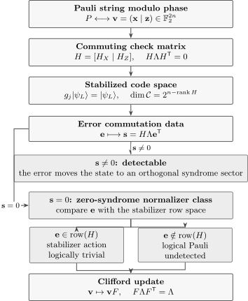
The stabilizer decision map in the row-vector convention. Commuting rows of $H$ define the code. An error vector $\mathbf e$ produces syndrome $\mathbf s=H\Lambda\mathbf e^{\mathsf T}$. A zero syndrome can mean either a stabilizer action, which is logically trivial, or an undetected logical operator. Clifford evolution preserves the same symplectic form.

Stabilizer Groups and Code Spaces

A qubit stabilizer group $S$ is an abelian subgroup of $\mathcal P_n$ such that

$$-I\notin S.$$

The stabilized subspace is

$$\begin{aligned} \mathcal C(S) = \big\{ |\psi\rangle:\;& g|\psi\rangle=|\psi\rangle \\ & \text{for every }g\in S \big\}. \end{aligned}$$

The exclusion of $-I$ is essential. If both $|\psi\rangle=-|\psi\rangle$ were required, the only solution would be the zero vector.

Suppose $S$ has $r$ independent commuting Hermitian generators,

$$S = \langle g_1,\ldots,g_r \rangle.$$

Independence means that no nonempty product of generators equals $I$. Every group element is a product

$$g_1^{a_1}\cdots g_r^{a_r}, \qquad a_j\in\mathbb F_2,$$

so

$$|S|=2^r.$$

The binary generator matrix

$$H = \left[ H_X\mid H_Z \right]$$

has one row per generator. Pairwise commutation is equivalent to

$$H\Lambda H^{\mathsf T}=0 \pmod2,$$

or

$$H_XH_Z^{\mathsf T} + H_ZH_X^{\mathsf T} = 0 \pmod2.$$

The row space is therefore an isotropic subspace of the binary symplectic vector space. Its rank cannot exceed $n$.

Projector and dimension

Each commuting generator contributes a $+1$-eigenspace projector:

$$\Pi_j = \frac{I+g_j}{2}.$$

Their product projects onto the common code space:

$$\begin{aligned} P_S &= \prod_{j=1}^r \frac{I+g_j}{2} \\ &= \frac{1}{2^r} \sum_{g\in S}g. \end{aligned}$$

Only the identity Pauli has nonzero trace, with $\operatorname{Tr}I=2^n$. Therefore

$$\begin{aligned} \dim\mathcal C(S) &= \operatorname{Tr}P_S \\ &= \frac{2^n}{2^r} \\ &= 2^{n-r}. \end{aligned}$$

An $[[n,k]]$ stabilizer code has

$$r=n-k$$

independent stabilizer generators. When $r=n$, the code space is one-dimensional and defines a pure stabilizer state. When $r<n$, it encodes $k=n-r$ logical qubits.

For a stabilizer state $|\psi\rangle$, the density operator has the compact expansion

$$|\psi\rangle\langle\psi| = \frac{1}{2^n} \sum_{g\in S}g.$$

For a code with $k>0$, the same expression is the maximally mixed encoded state:

$$\frac{P_S}{2^k} = \frac{1}{2^n} \sum_{g\in S}g.$$

Generator lists are not unique

Replacing a generator by its product with another generator does not change $S$. Binary row operations on $H$ therefore change the generating set while preserving the code. This freedom is useful for Gaussian elimination, measurement updates, and circuit design.

The abstract code may be unchanged, but generator choice can matter physically. Different generating sets can have different Pauli weights, geometrical supports, ancilla schedules, and fault-propagation behavior.

Worked Example: The Four-Qubit Detection Code

Consider four physical qubits with

$$\begin{aligned} g_X&=X_1X_2X_3X_4, \\ g_Z&=Z_1Z_2Z_3Z_4. \end{aligned}$$

The generators commute because they anticommute at four qubit positions. They are independent, so $r=2$ and

$$k=n-r=4-2=2.$$

The code is an $[[4,2,2]]$ stabilizer code. Its projector is

$$P = \frac14 \left( I+g_X+g_Z+g_Xg_Z \right).$$

Every one-qubit Pauli error anticommutes with at least one generator:

Error on any qubit $j$	syndrome $(s_X,s_Z)$
$X_j$	$(0,1)$
$Z_j$	$(1,0)$
$Y_j$	$(1,1)$

The code detects every single-qubit Pauli error. It does not locate the damaged qubit because all four $X_j$ errors, for example, have the same syndrome.

One valid choice of logical Pauli representatives is

$$\begin{aligned} \overline X_1&=X_1X_2, & \overline Z_1&=Z_2Z_3, \\ \overline X_2&=X_2X_3, & \overline Z_2&=Z_3Z_4. \end{aligned}$$

Each operator commutes with $g_X$ and $g_Z$. The designated logical pairs anticommute, while cross pairs commute. None belongs to $S$.

Because weight-$2$ logical Paulis exist and all weight-$1$ Paulis are detectable,

$$d=2.$$

The code detects one arbitrary qubit error and can correct one known-location erasure, but it cannot correct an arbitrary unknown-location one-qubit error. This is a useful warning: a nonzero syndrome can certify that an error occurred without providing enough information for deterministic recovery.

Logical Operators and the Pauli Normalizer

Let

$$\begin{aligned} C_{\mathcal P_n}(S) = \big\{ Q\in\mathcal P_n:\;& Qg=gQ \\ & \text{for every }g\in S \big\} \end{aligned}$$

be the Pauli centralizer of $S$. In stabilizer-code language this set is commonly called the Pauli normalizer $N(S)$. For the usual phase conventions, Pauli operators preserving the $+1$ code space must commute with every stabilizer.

There are three possibilities for a Pauli operator $Q$:

1. $Q$ anticommutes with some $g\in S$. It maps the code to an orthogonal syndrome sector.
2. $Q\in S$ up to phase. It acts trivially on every code state.
3. $Q\in N(S)\setminus S$ up to phase. It preserves the code but acts nontrivially on logical information.

The logical Pauli group is represented by the quotient

$$N(S)/S,$$

with global phases handled separately. For an $[[n,k]]$ code, one can choose representatives

$$\overline X_1,\ldots,\overline X_k, \qquad \overline Z_1,\ldots,\overline Z_k$$

that commute with every stabilizer and satisfy

$$\begin{aligned} \overline X_i\overline Z_j &= (-1)^{\delta_{ij}} \overline Z_j\overline X_i, \\ [\overline X_i,\overline X_j] &= 0, \\ [\overline Z_i,\overline Z_j] &= 0. \end{aligned}$$

Multiplying a logical representative by any stabilizer produces the same logical operation on the code:

$$\overline X_i \sim \overline X_i g, \qquad g\in S.$$

This equivalence is the algebraic source of stabilizer-code degeneracy.

Distance

For a stabilizer code,

$$d = \min_{Q\in N(S)\setminus S} \operatorname{wt}(Q),$$

where phases are ignored. The minimum undetectable nontrivial Pauli is precisely the minimum-weight logical Pauli.

The definition also explains why low-weight stabilizers do not reduce distance. A low-weight stabilizer is undetectable but logically trivial. Degenerate codes can therefore have stabilizers whose weight is below $d$.

Syndromes as Linear Algebra

Let an error Pauli have binary vector

$$\mathbf e = (\mathbf e_X\mid\mathbf e_Z).$$

Its syndrome against the $r$ generator rows is

$$\mathbf s = H\Lambda\mathbf e^{\mathsf T} \in \mathbb F_2^r.$$

Equivalently,

$$\mathbf s = H_X\mathbf e_Z^{\mathsf T} + H_Z\mathbf e_X^{\mathsf T} \pmod2.$$

The measured eigenvalue of generator $g_j$ is

$$(-1)^{s_j}$$

for an ideal code state after error $E$, because

$$g_jE|\psi_L\rangle = (-1)^{s_j} E|\psi_L\rangle.$$

The syndrome map is linear:

$$\mathbf s(\mathbf e+\mathbf f) = \mathbf s(\mathbf e) + \mathbf s(\mathbf f).$$

Two Pauli errors $E$ and $F$ have the same syndrome exactly when

$$E^\dagger F\in N(S)$$

up to phase. That fact divides same-syndrome pairs into two very different classes:

• if $E^\dagger F\in S$, the errors are degenerate and have the same logical action;
• if $E^\dagger F\in N(S)\setminus S$, they differ by a logical Pauli and cannot both be corrected by the same recovery.

A decoder therefore does not merely invert the syndrome map. It estimates an error equivalence class modulo stabilizers and must avoid choosing the wrong logical class. Decoders turns this algebraic statement into a posterior inference problem.

Knill–Laflamme in Stabilizer Language

The general exact-correction criterion is developed in Why Quantum Error Correction Is Possible. For a stabilizer code and a Pauli error set $\mathcal E$, it becomes especially concrete:

$$\begin{gathered} \mathcal E \text{ is correctable} \quad\Longleftrightarrow \\ E_a^\dagger E_b \notin N(S)\setminus S \end{gathered}$$

for every $E_a,E_b\in\mathcal E$, up to phase.

To see why, write $Q=E_a^\dagger E_b$.

If $Q$ anticommutes with a stabilizer $g$, then

$$\begin{aligned} P_SQP_S &= P_SgQP_S \\ &= -P_SQgP_S \\ &= -P_SQP_S, \end{aligned}$$

so

$$P_SQP_S=0.$$

The two errors occupy orthogonal syndrome sectors.

If $Q$ is a stabilizer up to phase, then

$$P_SQP_S = c_{ab}P_S.$$

The errors may share a syndrome, but they have the same action on the code.

Only the third case fails: if $Q\in N(S)\setminus S$, then $Q$ is a nontrivial logical Pauli, so $P_SQP_S$ is not proportional to $P_S$. The same syndrome has hidden a logical ambiguity.

This criterion is also the reason a distance-$d$ stabilizer code corrects arbitrary errors on

$$t \leq \left\lfloor \frac{d-1}{2} \right\rfloor$$

unknown qubits.

Clifford Operations

The $n$-qubit Clifford group is the normalizer of the Pauli group in the unitary group:

$$\mathcal C_n = \left\{ U: U\mathcal P_nU^\dagger = \mathcal P_n \right\}.$$

Thus a Clifford unitary maps every Pauli string to another Pauli string under conjugation. Standard generators are Hadamard, the phase gate $S$, and CNOT.

Gate	Pauli conjugation rules
$H_j$	$X_j\mapsto Z_j$, $Z_j\mapsto X_j$
$S_j$	$X_j\mapsto Y_j$, $Z_j\mapsto Z_j$
$\operatorname{CNOT}_{c\to t}$	$X_c\mapsto X_cX_t$, $Z_c\mapsto Z_c$, $X_t\mapsto X_t$, $Z_t\mapsto Z_cZ_t$
$\operatorname{CZ}_{a,b}$	$X_a\mapsto X_aZ_b$, $X_b\mapsto Z_aX_b$, both $Z$ operators fixed

Signs must be updated as well. For example,

$$HYH=-Y, \qquad SYS^\dagger=-X.$$

If $|\psi\rangle$ is stabilized by $S$, then $U|\psi\rangle$ is stabilized by

$$USU^\dagger = \left\{ UgU^\dagger: g\in S \right\}.$$

This is the stabilizer analogue of Heisenberg evolution: update a compact list of observables instead of expanding the state vector.

Binary Clifford action

Ignoring phases, Clifford conjugation induces a linear transformation

$$\mathbf v \longmapsto \mathbf vF$$

on binary row vectors. Commutation must be preserved, so

$$F\Lambda F^{\mathsf T} = \Lambda.$$

Such an $F$ is a binary symplectic matrix. The full Clifford operation requires both $F$ and phase data; the symplectic matrix alone cannot distinguish Cliffords that have the same action modulo Pauli signs.

Bell-state preparation by generator propagation

Start from $|00\rangle$, stabilized by

$$\langle Z_1,Z_2\rangle.$$

Apply $H_1$:

$$\langle Z_1,Z_2\rangle \longmapsto \langle X_1,Z_2\rangle.$$

Then apply $\operatorname{CNOT}_{1\to2}$:

$$\langle X_1,Z_2\rangle \longmapsto \langle X_1X_2,Z_1Z_2\rangle.$$

These are the generators of $|\Phi^+\rangle$. The computation never required writing its four amplitudes.

Code-preserving versus code-changing Cliffords

An arbitrary physical Clifford maps one stabilizer code to another code with conjugated stabilizer group. It implements a logical operation on the same code only when it preserves the code space, equivalently when

$$USU^\dagger=S.$$

It then maps logical Pauli representatives to logical Pauli representatives and induces a logical Clifford. A Clifford physical circuit is not automatically a valid fault-tolerant logical gate; error propagation and the code architecture still matter.

Pauli Measurement Updates

Let $M$ be a Hermitian Pauli observable with outcomes $m=\pm1$.

For a stabilizer code:

1. If $M\in S$, the outcome is deterministically $+1$.
2. If $-M\in S$, the outcome is deterministically $-1$.
3. If $M$ commutes with every stabilizer but $M\notin\pm S$, it acts as a logical Pauli. Measuring it generally reveals and disturbs logical information.
4. If $M$ anticommutes with at least one stabilizer, its expectation is zero for every code state, so ideal outcomes are equally likely. The measurement maps the state into a new stabilizer sector.

For the fourth case, choose a generator $g_j$ that anticommutes with $M$. Multiply every other generator that anticommutes with $M$ by $g_j$, making those rows commute with $M$. Then replace $g_j$ by

$$mM.$$

The updated generators commute and stabilize the postmeasurement state.

This algebraic rule describes an ideal Pauli measurement. A physical syndrome circuit must couple data to ancillas, read and reset them, repeat noisy checks, and prevent faults from spreading. Those circuit constructions belong to the syndrome-measurement and fault-tolerance pages.

Stabilizer Tableaus

A stabilizer tableau stores generator data as a binary matrix plus phase bits:

$$\left[ X \mid Z \mid \text{phase} \right].$$

For a pure $n$-qubit stabilizer state, one may track $n$ independent stabilizer rows. Simulation algorithms often add destabilizer rows or another canonical completion so that measurement outcomes and updates can be computed without repeating full Gaussian elimination.

The basic operations are:

• generator multiplication: binary row addition plus phase update;
• Clifford gate: local column and phase updates;
• Pauli measurement: commutation test, deterministic evaluation or random outcome, then row replacement;
• partial trace or mixed-state extension: reduce or augment the stored stabilizer data according to the chosen algorithm.

Storage is polynomial in $n$, rather than exponential in the number of qubits. Exact runtime depends on the tableau representation, operation sequence, sparsity, and requested output.

Gottesman–Knill Theorem

The Gottesman–Knill theorem states that circuits composed of:

• stabilizer-state preparations;
• Clifford gates;
• Pauli measurements;
• classical control conditioned on measurement outcomes;

can be simulated efficiently on a classical computer for standard sampling and stabilizer-tracking tasks.

The theorem remains striking because such circuits can generate large entangled states. Entanglement alone is therefore not sufficient for generic quantum computational hardness.

The theorem does not say:

• that every quantum circuit is efficiently simulable;
• that every property of a stabilizer circuit is trivial to compute under every input and output specification;
• that Clifford operations are useless experimentally;
• that an encoded Clifford circuit is automatically fault tolerant;
• that adding one non-Clifford gate to one circuit instance always makes simulation hard.

The closure mechanism is simple: Pauli descriptions remain Pauli descriptions. For example, the $T$ gate is non-Clifford because

$$TXT^\dagger = \frac{X+Y}{\sqrt2},$$

which is not proportional to a Pauli operator. Adding nonstabilizer states, non-Clifford gates, or non-Pauli measurements breaks the basic tableau closure, though specialized algorithms can still exploit a small amount of nonstabilizer structure.

What the Formalism Does Not Cover Automatically

Qudits

Prime-dimensional qudits admit a closely parallel construction using generalized shift and phase operators and symplectic linear algebra over a finite field. Composite dimensions require more careful modular arithmetic, phases, and module structure. The binary formulas on this page should not be copied unchanged to arbitrary $d$.

Subsystem codes

Subsystem stabilizer codes introduce a nonabelian gauge group. Only its center supplies stabilizer constraints, while gauge operators may be measured instead of high-weight stabilizers. Logical, gauge, and stabilizer equivalence classes must then be distinguished.

Bosonic and continuous-variable codes

Bosonic codes can have displacement-operator stabilizers or parity-like symmetries, but finite-energy states, unbounded operators, continuous syndromes, and oscillator noise require their own formalism. The qubit Pauli tableau is not a generic oscillator simulator.

General states and channels

Most pure states are not stabilizer states, and generic noisy channels do not map stabilizer states to stabilizer states. Pauli channels can be sampled inside stabilizer simulations, while coherent non-Clifford noise, amplitude damping, leakage, and correlated analog dynamics usually need additional representations or approximations.

Hardware and Decoder Interpretation

A stabilizer generator is an abstract Pauli observable. Hardware realizes it through a schedule of native interactions, ancillas, measurements, resets, and classical processing. The same abstract check can have several circuits with different:

• depth and connectivity;
• ancilla count;
• correlated-fault pathways;
• hook-error orientation;
• leakage behavior;
• readout latency;
• compatibility with simultaneous neighboring checks.

Likewise, a syndrome is not a correction. The decoder combines syndrome history with a noise model and boundary conditions to infer a likely logical equivalence class. Repeated measurements are needed because the syndrome bits themselves are noisy.

The formalism supplies exact algebraic invariants. Hardware claims require circuit-level noise, decoding, timing, and scaling evidence in addition.

A Stabilizer Audit

For any proposed stabilizer state, code, or circuit, record:

1. qubit ordering and Pauli convention;
2. generator signs and supports;
3. pairwise commutation;
4. generator rank and exclusion of $-I$;
5. code dimension $2^{n-r}$;
6. logical Pauli representatives and their commutation relations;
7. distance or a clearly limited detected-error set;
8. syndrome convention and bit ordering;
9. Clifford conjugation and phase rules;
10. measurement update convention;
11. decoder assumptions and equivalence classes;
12. physical circuit and fault model if an implementation is claimed.

This checklist catches most sign, rank, and logical-operator mistakes before they become decoder or circuit bugs.

Common Mistakes

• Omitting Pauli phases from the group, then using a set that is not closed under multiplication.
• Dropping generator signs even though $g$ and $-g$ select opposite eigenspaces.
• Allowing noncommuting generators or including $-I$.
• Counting listed generators instead of their binary rank.
• Treating a generator list as unique.
• Confusing a stabilizer state, with $k=0$, and a stabilizer code, with $k>0$.
• Calling every zero-syndrome Pauli harmless. Elements of $N(S)\setminus S$ are logical errors.
• Assuming errors with the same syndrome are always degenerate.
• Forgetting that binary vectors omit phase information.
• Calling an arbitrary physical Clifford a logical gate on a fixed code.
• Saying a distance-$d$ code corrects $d-1$ unknown-location errors.
• Interpreting efficient stabilizer simulation as evidence that entanglement or Clifford control is physically easy.
• Applying binary qubit formulas unchanged to composite-dimensional qudits or bosonic modes.

Exercises

1. Symplectic commutation test

Represent

$$P=X_1Z_2Y_3, \qquad Q=Z_1X_2$$

as binary vectors and determine whether they commute.

Solution

For $P$,

$$\mathbf x_P=(1,0,1), \qquad \mathbf z_P=(0,1,1).$$

For $Q$,

$$\mathbf x_Q=(0,1,0), \qquad \mathbf z_Q=(1,0,0).$$

The symplectic product is

$$\begin{aligned} \omega(P,Q) &= \mathbf x_P\cdot\mathbf z_Q + \mathbf z_P\cdot\mathbf x_Q \\ &= 1+1 \\ &= 0 \pmod2. \end{aligned}$$

The strings commute. Directly, they anticommute on qubits 1 and 2, giving two minus signs, and commute on qubit 3.

2. Projector and code dimension

Let $S=\langle g_1,g_2,g_3\rangle$ be generated by three independent commuting nonidentity Paulis on five qubits, with $-I\notin S$. Write the code projector and find the number of encoded qubits.

Solution

The projector is

$$\begin{aligned} P_S &= \prod_{j=1}^3 \frac{I+g_j}{2} \\ &= \frac18 \sum_{g\in S}g. \end{aligned}$$

There are $r=3$ independent checks on $n=5$ qubits, so

$$\dim\mathcal C = 2^{5-3} = 4.$$

The code encodes

$$k=5-3=2$$

logical qubits.

3. Four-qubit syndromes

For the code generated by

$$g_X=XXXX, \qquad g_Z=ZZZZ,$$

compute the syndromes of $X_3$, $Y_3$, and $Z_3$ in the order $(g_X,g_Z)$.

Solution

$X_3$ commutes with $g_X$ and anticommutes with $g_Z$, so

$$\mathbf s(X_3)=(0,1).$$

$Z_3$ anticommutes with $g_X$ and commutes with $g_Z$, so

$$\mathbf s(Z_3)=(1,0).$$

$Y_3$ anticommutes with both, so

$$\mathbf s(Y_3)=(1,1).$$

The result is independent of the qubit index. The syndrome identifies the Pauli type in this one-fault set but not its location.

4. Check the logical Pauli representatives

For the same code, verify that

$$\begin{aligned} \overline X_1&=X_1X_2, & \overline Z_1&=Z_2Z_3, \\ \overline X_2&=X_2X_3, & \overline Z_2&=Z_3Z_4 \end{aligned}$$

have the required logical commutation relations.

Solution

Every listed operator has even overlap between its $X$ support and the support of $g_Z$, or between its $Z$ support and $g_X$. Hence all commute with both stabilizers.

$\overline X_1$ and $\overline Z_1$ overlap with different nonidentity Pauli factors only on qubit 2, so they anticommute. Likewise, $\overline X_2$ and $\overline Z_2$ overlap only on qubit 3 and anticommute.

The cross pair $\overline X_1,\overline Z_2$ has no conflicting overlap, so it commutes. The cross pair $\overline X_2,\overline Z_1$ has conflicting overlap on qubits 2 and 3, giving two minus signs, so it also commutes. Same-type logical operators commute.

All representatives have weight $2$ and none is a stabilizer. Since every weight-$1$ Pauli is detected, this also confirms $d=2$.

5. Orthogonal syndrome sectors

Let $Q$ anticommute with some stabilizer $g$. Prove that

$$P_SQP_S=0.$$

Solution

Because $g$ stabilizes the code,

$$gP_S=P_Sg=P_S.$$

Using $gQ=-Qg$,

$$\begin{aligned} P_SQP_S &= P_SgQP_S \\ &= -P_SQgP_S \\ &= -P_SQP_S. \end{aligned}$$

The only operator equal to its negative is zero, so

$$P_SQP_S=0.$$

This is the stabilizer proof that different syndromes define orthogonal error sectors.

6. Bell state by Clifford propagation

Propagate the stabilizers of $|00\rangle$ through $H_1$ followed by $\operatorname{CNOT}_{1\to2}$.

Solution

Initially,

$$S_0=\langle Z_1,Z_2\rangle.$$

Hadamard conjugates $Z_1$ to $X_1$:

$$S_1=\langle X_1,Z_2\rangle.$$

CNOT propagates control $X$ to both qubits and target $Z$ to both qubits:

$$S_2 = \langle X_1X_2, Z_1Z_2 \rangle.$$

The unique simultaneous $+1$ eigenstate is

$$|\Phi^+\rangle = \frac{|00\rangle+|11\rangle}{\sqrt2}.$$

7. Pauli measurement update

Start from $|00\rangle$ with stabilizers $\langle Z_1,Z_2\rangle$ and measure $M=X_1X_2$. Find updated generators for outcomes $m=\pm1$ and identify the postmeasurement states.

Solution

$M$ anticommutes with both $Z_1$ and $Z_2$. Choose $g_1=Z_1$. Replace the other anticommuting generator by

$$g_2' = Z_1Z_2,$$

which commutes with $M$. Replace $g_1$ by $mM$. The updated stabilizer group is

$$\langle mX_1X_2, Z_1Z_2 \rangle.$$

For $m=+1$, the state is

$$|\Phi^+\rangle = \frac{|00\rangle+|11\rangle}{\sqrt2}.$$

For $m=-1$, the state is

$$|\Phi^-\rangle = \frac{|00\rangle-|11\rangle}{\sqrt2}.$$

Each outcome has probability $1/2$.

8. Same syndrome, different logical class

In the $[[4,2,2]]$ code, show that $X_1$ and $X_2$ have the same syndrome but cannot both be corrected by one syndrome-conditioned recovery.

Solution

Both errors commute with $g_X$ and anticommute with $g_Z$, so each has syndrome

$$(0,1).$$

Their relative product is

$$X_1^\dagger X_2 = X_1X_2 = \overline X_1.$$

This operator belongs to $N(S)\setminus S$ and acts as a nontrivial logical Pauli. If one recovery corrects $X_1$, applying that same recovery after $X_2$ leaves a logical $\overline X_1$ error, or vice versa. Equal syndromes are safe only when the relative product is a stabilizer, not a logical operator.

9. A non-Clifford test

Explain why

$$TXT^\dagger = \frac{X+Y}{\sqrt2}$$

proves that $T$ is not a Clifford gate.

Solution

A Clifford unitary must map every Pauli operator to another Pauli operator under conjugation. The operator

$$\frac{X+Y}{\sqrt2}$$

is a coherent linear combination of two distinct Pauli matrices and is not proportional to $I$, $X$, $Y$, or $Z$. Therefore $T$ does not normalize the Pauli group and is non-Clifford.

Further Connections

• Why Quantum Error Correction Is Possible
• Surface Code
• Stabilizer Simulation develops implementation choices, bit-packed tableaus, batched Pauli frames, detector streams, decoder interfaces, logical-error experiments, and simulator validation.
• Stabilizer States Preview
• Graph States
• Multi-Qubit Gates
• Universal Gate Sets
• Circuit Optimization applies Pauli commutation, symplectic maps, tableaux, and Clifford resynthesis to circuit simplification.
• Stabilizer Identities
• Stabilizer Circuit
• Pauli Matrix Table

References

• D. Gottesman, Stabilizer Codes and Quantum Error Correction, Ph.D. thesis, California Institute of Technology, 1997, doi:10.7907/rzr7-dt72, arXiv:quant-ph/9705052.
• D. Gottesman, “Class of quantum error-correcting codes saturating the quantum Hamming bound,” Physical Review A 54, 1862–1868, 1996, doi:10.1103/PhysRevA.54.1862.
• A. R. Calderbank, E. M. Rains, P. W. Shor, and N. J. A. Sloane, “Quantum error correction and orthogonal geometry,” Physical Review Letters 78, 405–408, 1997, doi:10.1103/PhysRevLett.78.405.
• E. Knill and R. Laflamme, “Theory of quantum error-correcting codes,” Physical Review A 55, 900–911, 1997, doi:10.1103/PhysRevA.55.900.
• D. Gottesman, “The Heisenberg representation of quantum computers,” in Group22: Proceedings of the XXII International Colloquium on Group Theoretical Methods in Physics, 1999, arXiv:quant-ph/9807006.
• J. Dehaene and B. De Moor, “Clifford group, stabilizer states, and linear and quadratic operations over GF(2),” Physical Review A 68, 042318, 2003, doi:10.1103/PhysRevA.68.042318.
• S. Aaronson and D. Gottesman, “Improved simulation of stabilizer circuits,” Physical Review A 70, 052328, 2004, doi:10.1103/PhysRevA.70.052328.
• E. Hostens, J. Dehaene, and B. De Moor, “Stabilizer states and Clifford operations for systems of arbitrary dimensions and modular arithmetic,” Physical Review A 71, 042315, 2005, doi:10.1103/PhysRevA.71.042315.
• D. Gottesman, “An introduction to quantum error correction and fault-tolerant quantum computation,” in Quantum Information Science and Its Contributions to Mathematics, Proceedings of Symposia in Applied Mathematics 68, 13–58, 2010, arXiv:0904.2557.
• B. M. Terhal, “Quantum error correction for quantum memories,” Reviews of Modern Physics 87, 307–346, 2015, doi:10.1103/RevModPhys.87.307.
• M. A. Nielsen and I. L. Chuang, Quantum Computation and Quantum Information, 10th anniversary ed., Cambridge University Press, 2010, doi:10.1017/CBO9780511976667.
• J. Preskill, Quantum Error Correction, Chapter 7 of the Caltech quantum computation lecture notes, updated 2026, course materials.

Summary

The stabilizer formalism replaces generic amplitude bookkeeping by Pauli constraints. Binary symplectic vectors encode Pauli support and commutation; an abelian group with $r$ independent generators defines a $2^{n-r}$-dimensional code; the Pauli normalizer supplies logical operators; and syndromes are linear commutation data.

Clifford gates preserve this structure, Pauli measurements update it by generator replacement, and tableaus make the resulting subtheory classically tractable. For error correction, the decisive distinction is among detectable operators, stabilizers that act trivially, and zero-syndrome logical operators. That distinction turns the general Knill–Laflamme theorem into an exact algebraic test for stabilizer codes.