Circuit Optimization

Short Definition

Circuit optimization transforms an existing quantum or quantum–classical circuit into a circuit with the same declared behavior and lower cost under a stated objective. The transformation may cancel inverse gates, fuse rotations, commute operations to expose cancellations, resynthesize small windows, exploit Clifford or phase-polynomial structure, shorten a dependency graph, or search a larger equivalence class. It is not merely “removing gates”: an optimizer can deliberately add gates or ancillas to reduce depth, non-Clifford cost, duration, or another more important resource.

A complete contract has the schematic form

$$\mathsf{Optimize} \bigl( C;\, \mathcal E,\, \mathcal G,\, \mathcal A,\, \mathbf c,\, \mathcal B \bigr) \longrightarrow \bigl( C',\, \mathcal K \bigr).$$

Here $C$ is the input circuit, $\mathcal E$ defines behavioral equivalence, $\mathcal G$ is the legal operation set, $\mathcal A$ is the ancilla and classical-control contract, $\mathbf c$ is the cost model, and $\mathcal B$ contains limits on compiler time, memory, and approximation. The output $C'$ comes with a certificate $\mathcal K$ identifying the transformations, equivalence evidence, costs, assumptions, and tool versions.

This page is the canonical home for circuit rewriting, simplification, commutation, and abstract depth reduction. Gate Decomposition owns synthesis of an operation into a gate alphabet. Circuit Intermediate Representations owns the representation and capability contract. Later pages in this chapter own logical-to-physical placement, routing, calibration- and noise-aware choices, and pulse scheduling. A compiler may interleave those tasks, but their claims and evidence remain distinct.

Optimization Begins with Semantics

For a static unitary circuit on the same input and output wires, a common exact contract is

$$U(C') = e^{i\phi}U(C),$$

where a global phase is allowed only if the surrounding context makes it unobservable. If the block can later be controlled, used on one interferometer branch, or compared with a phase reference, literal equality or an explicitly propagated phase correction may be required.

Approximate optimization must name both metric and budget. One possible contract is

$$\min_{\phi\in\mathbb R} \left\| U(C')-e^{i\phi}U(C) \right\|_{\mathrm{op}} \leq \epsilon_{\mathrm{opt}}.$$

Near-equality is not an automatic license to delete a small rotation. It is a different compiler mode whose error must be composed with algorithmic, synthesis, numerical, and physical error budgets. Error Estimates develops the distinction between a residual, a bound, and a certified tolerance.

Unitary equality is insufficient for dynamic circuits. Measurements, resets, discarded systems, and classical branches define a channel or, when outcomes are retained, a quantum instrument. If $\mathcal I_y^C$ is the trace-nonincreasing map associated with output record $y$, exact instrument-level equivalence asks for

$$\begin{aligned} \mathcal I_y^{C'}(\rho) &= \mathcal I_y^C(\rho), \\ &\text{for all }\rho\text{ and retained }y. \end{aligned}$$

This requirement preserves both $p(y|\rho)=\operatorname{Tr}\mathcal I_y^C(\rho)$ and the conditional output state. Preserving only the outcome distribution is weaker; preserving only the unconditioned channel is weaker still. Quantum Instruments is the canonical treatment of these distinctions.

Ancillas introduce another boundary. An exact clean-ancilla rewrite may need

$$U(C') \bigl( |\psi\rangle\otimes|0^a\rangle \bigr) = e^{i\phi} U(C) |\psi\rangle\otimes|0^a\rangle$$

for every data state $|\psi\rangle$, including restoration of all $a$ ancillas. Equality only on computational-basis inputs, or only after tracing out garbage, is a different contract and cannot be substituted silently.

Cost Is a Vector

Useful circuit costs are rarely ordered by a single universal number. A target-independent optimizer might retain

$$\begin{aligned} \mathbf c(C) = \bigl(& N_{2q},\, D_{2q},\, N_T,\, D_T, \\ & N_{1q},\, D,\, N_{\mathrm{anc}},\, N_{\mathrm{meas}},\, \tau_{\mathrm{comp}} \bigr), \end{aligned}$$

where $N$ denotes counts, $D$ denotes abstract depths, and $\tau_{\mathrm{comp}}$ is compiler runtime. A present-day device may care most about entanglers and duration. A fault-tolerant architecture may prioritize magic-state demand, reaction depth, or spacetime volume. A simulator may prefer gates that admit efficient fusion even when the emitted circuit is not best for hardware.

There are three defensible ways to compare cost vectors:

1. a lexicographic policy, such as minimizing $T$ count before Clifford count;
2. a weighted score whose units and weights are recorded;
3. a Pareto policy that retains every nondominated candidate.

The statement “$C'$ is optimized” is incomplete without one of these choices. Even “minimum depth” is ambiguous until gate durations, concurrency, resource conflicts, measurement latency, and connectivity are fixed.

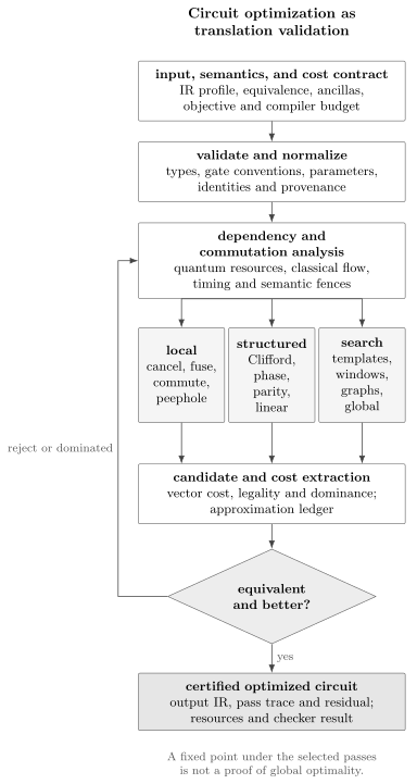
Optimization is a translation-validation loop. Candidate rewrites are accepted only when they satisfy the declared equivalence and improve the selected cost policy. Rejected or dominated candidates return to pass selection; accepted circuits retain a pass trace and certificate.

Expose the Dependency Structure

A textual gate list contains an arbitrary choice of order among operations that could run or move independently. Optimizers therefore construct a dependency directed acyclic graph

$$D_C = \bigl( V,\, E_q\cup E_c\cup E_t\cup E_f \bigr),$$

where vertices are operations and edges encode quantum-resource order, classical data flow, timing constraints, and semantic fences. Every legal schedule is a topological ordering that also satisfies the target capability contract.

Operations on disjoint subsystems commute. Operations sharing a subsystem may also commute, but this must follow from their semantics rather than their diagrammatic appearance. For unitary gates $A$ and $B$,

$$AB=BA \quad\Longleftrightarrow\quad [A,B]=0.$$

For Pauli strings, write a Pauli modulo phase as $P(\mathbf a,\mathbf b)$ with $X$ support $\mathbf a$ and $Z$ support $\mathbf b$. Then

$$\begin{aligned} P(\mathbf a,\mathbf b) P(\mathbf c,\mathbf d) &= (-1)^\omega P(\mathbf c,\mathbf d) P(\mathbf a,\mathbf b), \\ \omega &= \mathbf a\mathbin{\cdot}\mathbf d + \mathbf b\mathbin{\cdot}\mathbf c \pmod 2. \end{aligned}$$

The strings commute exactly when $\omega=0$. Their rotations then commute as well:

$$\begin{aligned} \omega=0 &\quad\Longrightarrow\quad R_P(\alpha)R_Q(\beta) \\ &= R_Q(\beta)R_P(\alpha). \end{aligned}$$

Gate-specific commutation rules are often cheaper to check. For $\operatorname{CNOT}_{c\to t}$,

$$\begin{aligned} \operatorname{CNOT}_{c\to t}R_{z,c}(\theta) &= R_{z,c}(\theta)\operatorname{CNOT}_{c\to t}, \\ \operatorname{CNOT}_{c\to t}R_{x,t}(\theta) &= R_{x,t}(\theta)\operatorname{CNOT}_{c\to t}. \end{aligned}$$

The analogous $R_{z,t}$ and $R_{x,c}$ moves are not generally valid. A rewrite engine should encode the positive rule and its side conditions, not infer a visual symmetry that the gate does not possess.

Barriers require a declared meaning. A semantic fence forbids movement because an external timing, calibration, or observation contract depends on the boundary. A display-only barrier may be ignored. Treating both spellings as the same object either blocks useful work or changes behavior.

Local Simplification and Canonicalization

The cheapest passes remove algebraic redundancy:

$$\begin{aligned} GG^\dagger &= I, \\ R_P(\alpha)R_P(\beta) &= R_P(\alpha+\beta), \\ R_P(0) &= I. \end{aligned}$$

This includes deleting identities, canceling adjacent self-inverse gates, fusing rotations about the same Pauli axis, normalizing angles, removing dead classical calculations, and canonicalizing equivalent gate spellings. A commutation pass can bring matching operations together before the local rule fires.

Angle normalization must respect the equivalence contract. With

$$R_P(\theta) = e^{-i\theta P/2},$$

one has

$$\begin{aligned} R_P(\theta+2\pi) &= -R_P(\theta), \\ R_P(\theta+4\pi) &= R_P(\theta). \end{aligned}$$

Reduction modulo $2\pi$ is valid up to global phase for an isolated unitary, but modulo $4\pi$ is needed for literal matrix equality. The sign can become a relative phase after adding a control. Canonicalization is therefore not semantics-free bookkeeping.

Local rules should also preserve parameter domains. The exact symbolic rule

$$\begin{aligned} & R_z(a\theta+b)R_z(c\theta+d) \\ &\qquad= R_z\bigl((a+c)\theta+b+d\bigr) \end{aligned}$$

holds for every allowed $\theta$. Replacing a rotation because its angle is small at one sampled parameter value is approximate specialization, not symbolic optimization.

Worked example: merge two parity rotations

Writing $C_{12}=\operatorname{CNOT}_{1\to2}$, the standard decomposition

$$\mathcal Z_{12}(\theta) = e^{-i\theta Z_1Z_2/2} = C_{12} R_{z,2}(\theta) C_{12}$$

can arise twice in succession. Expanding both blocks gives

$$\begin{aligned} \mathcal Z_{12}(\alpha) \mathcal Z_{12}(\beta) &= C_{12} R_z(\alpha) C_{12} \\ &\quad{}\times C_{12} R_z(\beta) C_{12} \\ &= C_{12} R_z(\alpha+\beta) C_{12} \\ &= \mathcal Z_{12}(\alpha+\beta). \end{aligned}$$

The middle CNOTs cancel and the rotations fuse. The result reduces four entanglers to two, or to zero when $\alpha+\beta$ is an allowed identity angle. This example also shows why pass order matters: expanding structured operations can expose a cancellation, while expanding too early can hide larger algebraic structure.

Peepholes, Templates, and Superoptimization

A peephole optimizer selects a small subcircuit $W$, computes or recognizes its semantics, and replaces it by a cheaper equivalent $W'$. Exact matrix comparison is practical only for small wire counts, but a window can also be classified by a Clifford tableau, binary linear map, phase polynomial, or another compact invariant.

Template methods begin with an identity

$$T = G_0G_1\cdots G_{m-1} \simeq I.$$

If commutation and pattern matching identify a costly product $A$ from this template inside the circuit, the relation $AB\simeq I$ implies

$$A \simeq B^\dagger.$$

Replacing $A$ by $B^\dagger$ is profitable when the chosen cost of $B$ is smaller and every side condition is satisfied. Templates can reach beyond adjacent cancellation while remaining interpretable and fast.

Window resynthesis searches more broadly. It may enumerate circuits up to a size bound, use meet-in-the-middle tables, invoke a canonical synthesizer, or apply numerical optimization to a parameterized ansatz. Superoptimization extends this idea by generating equivalence classes or candidate identities and searching them under a cost model. Because exhaustive search grows rapidly, practical systems restrict width, gate count, parameter form, or search time.

Rewrite direction needs a termination policy. If every accepted exact rule strictly decreases a well-founded lexicographic score, repeated rewriting terminates, though possibly at a poor local minimum. Bidirectional rules such as commutation can loop. Equality-saturation systems avoid committing to one direction by storing many equivalent forms and performing cost extraction later, but their equivalence graph can itself grow beyond practical limits.

Exploit Algebraic Structure

Local matrices are not the only useful semantics. Different circuit fragments admit different compact descriptions.

Fragment	Compact semantics	Typical optimization
CNOT network	invertible binary matrix	block resynthesis and Gaussian-style elimination
CNOT plus diagonal phases	linear map plus phase polynomial	parity-term fusion and resynthesis
Clifford circuit	symplectic map and phase data	tableau reduction and Clifford resynthesis
Pauli rotations	labeled Pauli strings and angles	commuting sets, phase gadgets, shared parity networks
reversible classical circuit	basis-state permutation or Boolean map	templates and reversible-logic resynthesis
general bounded-width window	dense unitary or channel	exact or approximate peephole search
ZX diagram	typed open graph with rewrite semantics	graph simplification and circuit extraction

The optimizer should move into a representation whose equality test and rewrite rules match the fragment, then return with a checked extraction procedure. No one representation makes every optimization easy.

Linear reversible blocks

A CNOT-only circuit acts on computational-basis strings as

$$|x\rangle \longmapsto |Ax\rangle, \qquad A\in GL(n,\mathbb F_2).$$

Each CNOT is an elementary row operation over $\mathbb F_2$. An optimizer can accumulate a maximal block into $A$ and resynthesize the map rather than preserve an inefficient historical sequence. On unrestricted connectivity, the worst-case CNOT count can be made $\Theta(n^2/\log n)$, asymptotically improving ordinary one-row-at-a-time elimination. Connectivity-constrained synthesis belongs with mapping and routing; the algebraic target $A$ should be retained for that later pass.

Phase polynomials

Let

$$\Phi(\alpha) = \operatorname{diag}(1,e^{i\alpha}).$$

A circuit over CNOT and these phase gates acts as

$$C|x\rangle = e^{if(x)} |Ax\rangle,$$

where $A\in GL(n,\mathbb F_2)$ and

$$f(x) = \sum_{j=1}^{m} \alpha_j\ell_j(x) \pmod{2\pi}.$$

Each $\ell_j:\mathbb F_2^n\to\mathbb F_2$ is a parity function, embedded as $0$ or $1$ in the phase. A CNOT updates the live parity labels; a phase gate adds its angle to the label currently carried by its wire. Terms with the same $\ell_j$ can be combined, and a coefficient equal to zero modulo $2\pi$ disappears.

This representation sees cancellations separated by long CNOT networks. It also distinguishes the final linear transformation $A$ from the phase function $f$, so either part can be resynthesized. Since

$$\Phi(\alpha) = e^{i\alpha/2}R_z(\alpha),$$

converting between phase-gate and $R_z$ conventions requires tracking global phase whenever the context is phase-sensitive.

For Clifford+$T$ circuits, coefficients are multiples of $\pi/4$. Odd coefficients represent non-Clifford phase terms, while even coefficients are Clifford phases. Reducing the number or layering of odd terms can lower $T$ count or $T$ depth. For important diagonal families, $T$-count reduction is related to decoding punctured Reed–Muller codes; more generally, common gate-count and depth optimization problems are NP-hard. Efficient heuristics and restricted exact algorithms are therefore central, not temporary substitutes for a known universal polynomial-time optimizer.

Clifford and Pauli structure

A Clifford circuit maps Paulis to Paulis under conjugation, so its action can be stored as a binary symplectic transformation plus phase data. Large Clifford windows can then be compared and resynthesized without constructing a $2^n\times2^n$ matrix. Stabilizer Formalism develops the tableau and symplectic representation.

Circuits dominated by Pauli rotations benefit from grouping commuting strings, combining identical rotations, and sharing parity-computation networks. A phase gadget represents a parity-dependent phase independently of one particular CNOT ladder. Keeping the gadget abstract allows a later extractor to trade entangler count against depth or connectivity.

ZX-calculus

The ZX-calculus translates circuits into open diagrams whose sound rewrite rules can expose nonlocal Clifford and phase structure. Graph transformations such as local complementation and pivoting can simplify a diagram before a new circuit is extracted. This can reveal cancellations hidden from fixed-width peepholes.

Three claims must remain separate:

• every applied graphical rewrite is sound in the declared fragment;
• the chosen rewrite strategy reaches a useful reduced diagram;
• circuit extraction succeeds and improves the selected circuit cost.

Soundness does not imply that a heuristic finds a global optimum, and a smaller diagram need not extract to a cheaper circuit under every gate alphabet. Completeness is also fragment-dependent. The certificate should record the rule set, scalar convention, extraction algorithm, and post- extraction cost.

Depth Reduction and Scheduling

For a dependency graph with operation duration $d(v)$, an abstract critical path is

$$D(C) = \max_{\pi\in\operatorname{Paths}(D_C)} \sum_{v\in\pi}d(v).$$

Taking $d(v)=1$ gives layer depth; assigning gate-class durations gives a weighted depth. An as-soon-as-possible schedule supplies an upper bound after resource conflicts are included, while an as-late-as-possible schedule reveals slack. Commutation can remove avoidable order edges, and resynthesis can change the graph itself.

Count and depth can move in opposite directions. Parallelizing parity computations may require more ancillas or CNOTs. Minimizing $T$ depth can leave $T$ count unchanged and increase Clifford work. A target-independent depth claim should therefore state:

• operation durations or the unit-layer convention;
• which operations conflict for resources;
• whether classical feedforward has zero or nonzero latency;
• whether connectivity and movement are included;
• whether ancillas may be introduced.

Physical placement, routing, crosstalk, calibrated durations, and controller timing can reverse an abstract schedule. Those refinements belong to their later canonical pages.

Pass Ordering and Fixed Points

Optimization passes generally do not commute:

$$\mathcal O_2\!\left(\mathcal O_1(C)\right) \neq \mathcal O_1\!\left(\mathcal O_2(C)\right).$$

Rotation fusion before finite-alphabet synthesis can approximate one angle instead of two. Decomposition can expose adjacent inverses. Local cleanup can make a larger resynthesis window recognizable. Routing can introduce SWAP or direction-correction gates that create new local cancellations. Conversely, premature decomposition can erase a high-level operation that a structure-aware pass would optimize better.

A robust pipeline commonly alternates:

1. validation and canonical normalization;
2. inexpensive local cleanup;
3. dependency and commutation analysis;
4. structure-specific block optimization;
5. bounded global or window search;
6. cleanup and cost extraction;
7. translation validation.

Repeating passes to a fixed point is useful only with a stop rule. Record the iteration bound, score history, timeout, random seed, and whether the final candidate is deterministic. A fixed point under one pass set means only that those passes found no accepted rewrite; it is not a proof of global optimality.

Parameterized and Approximate Circuits

Parameterized circuits require identities valid on the declared parameter domain. An optimizer may:

• combine affine angle expressions exactly;
• propagate known periodicities and constants;
• factor shared parameter expressions;
• use commutation conditions independent of parameter values;
• specialize only after parameters are bound.

Numerical sampling of several parameter values is not proof of a symbolic identity. Branch cuts in Euler angles, floating-point comparisons near multiples of $2\pi$, and assumptions such as $\theta\neq0$ should be explicit. For variational workloads, an approximate rewrite can also alter derivatives and the objective landscape even when sampled unitaries are close.

Approximate block replacement should return a residual in a composable metric. If unitary replacements satisfy

$$\left\| U_j-V_j \right\|_{\mathrm{op}} \leq \epsilon_j,$$

then a telescoping argument gives the conservative bound

$$\left\| U_m\cdots U_1 - V_m\cdots V_1 \right\|_{\mathrm{op}} \leq \sum_{j=1}^{m}\epsilon_j.$$

This bound may be loose, but it prevents an optimizer from spending the same global tolerance independently in every window. Gate Decomposition owns synthesis-error allocation and finite-alphabet approximation.

Measurements, Resets, and Classical Control

Dynamic operations break many unitary intuitions:

• measurement is not invertible, so it has no cancellation partner;
• reset discards input information and is not an inverse of preparation;
• moving a gate through measurement can change the measured observable;
• branch-local rewrites must preserve classical labels and branch conditions;
• dead-branch elimination needs a proof that the condition is unreachable;
• moving work across a feedback boundary can change latency and noise exposure.

For example, applying $X$ before a computational-basis measurement flips the outcome distribution. Moving it after measurement is equivalent only if the classical bit is also negated and no retained post-measurement quantum state requires the original action. This is an instrument rewrite with a classical relabeling, not ordinary gate commutation.

Compiler IRs should expose quantum and classical dependencies, measurement result ownership, reset postconditions, and semantic fences. Optimizing only a drawn unitary skeleton can silently invalidate an adaptive program.

Verification and Certificates

Optimization is unusually well suited to translation validation: verify the particular input–output pair produced by a pass, even when the optimizer itself is not formally proved correct.

For static unitary circuits on modest width, form the miter

$$M = U(C')^\dagger U(C).$$

Exact phase-insensitive equivalence requires $M=e^{i\phi}I$. Full matrices are exponential, so larger circuits need structure-aware methods: Clifford tableaux, phase polynomials, path sums, decision diagrams, tensor contraction, ZX reduction, symbolic algebra, or proof-assistant-verified rewrite rules. Each method has a scope and can return “unknown” without showing non-equivalence.

Use layered evidence:

1. prove each primitive rewrite once, including side conditions;
2. validate IR invariants before and after every pass;
3. check compact semantic invariants for structured fragments;
4. translation-validate the actual emitted circuit;
5. use full matrices only for bounded width;
6. run randomized state tests as diagnostics, not proofs;
7. retain an independently checkable certificate where practical.

A useful optimization record includes:

Field	Minimum content
input	circuit hash, IR version, gate definitions, parameter bindings
equivalence	unitary, phase-insensitive, subspace, channel, instrument, or approximate
resources	ancilla initialization and restoration, classical outputs, fences
objective	full cost vector, ordering policy, durations and connectivity assumptions
passes	ordered pass list, parameters, iterations, implementation versions
search	timeout, random seed, candidate budget, optimality claim if any
validation	checker, semantic representation, precision, residual, result
output	circuit hash, resource counts, depth model, provenance map

Formal verification does not certify the physical device. It certifies a relation between modeled artifacts. Calibration drift, crosstalk, leakage, controller faults, and model mismatch require separate experimental evidence.

Common Mistakes

• Reporting “gate-count reduction” without naming the gate alphabet and counted gate classes.
• Treating a lower count as a lower depth, duration, or logical cost.
• Canceling gates that are adjacent in text but separated by a classical, timing, or resource dependency.
• Commuting through a measurement or reset using a unitary identity alone.
• Reducing $R_P$ angles modulo $2\pi$ when literal phase matters.
• Using a floating-point near-zero test as an exact symbolic rewrite.
• Dropping or borrowing ancillas without preserving their state contract.
• Assuming a local fixed point is globally optimal.
• Comparing optimizer benchmarks with different decomposition, routing, timeout, or verification settings.
• Running an optimization pass without updating provenance and approximation budgets.
• Treating successful random simulation as an equivalence proof.
• Calling a hardware-noise score “fidelity” without a calibrated model and validation data.

Exercises

1. Fuse rotations with the correct period

Simplify $R_z(\alpha)R_z(\beta)$ and state when an angle may be reduced modulo $2\pi$ rather than $4\pi$.

Solution

The generators are identical, so their exponentials commute and combine:

$$R_z(\alpha)R_z(\beta) = R_z(\alpha+\beta).$$

Because $R_z(\theta+2\pi)=-R_z(\theta)$, reduction modulo $2\pi$ preserves the operation only up to global phase. It is valid when the equivalence contract quotients global phase and the block cannot later be controlled or placed in a phase-sensitive context. Literal matrix equality uses period $4\pi$.

2. Test Pauli commutation

Determine whether $P=X_1Y_2Z_4$ commutes with $Q=Z_1Y_2X_3$, and decide whether their rotations may be reordered.

Solution

On qubit $1$, $X$ and $Z$ anticommute. On qubit $2$, the two $Y$ operators commute. On qubit $3$, $P$ is identity, and on qubit $4$, $Q$ is identity. There is one anticommuting overlap, so

$$PQ=-QP.$$

The strings do not commute, and generic rotations $R_P(\alpha)$ and $R_Q(\beta)$ cannot be reordered. Special angles can produce accidental identities, but they require a separate parameter-aware proof.

3. Optimize two ZZ gadgets

Starting from the decomposed circuit for $\mathcal Z_{12}(\alpha)\mathcal Z_{12}(-\alpha)$, count the CNOTs before and after local optimization.

Solution

Each gadget initially contains two CNOTs, so the concatenation has four. The two middle CNOTs cancel. The remaining rotations fuse:

$$R_z(\alpha)R_z(-\alpha)=I.$$

The two outer CNOTs then become adjacent and cancel. The optimized circuit is the identity with zero CNOTs. The result is exact, including global phase, because $\mathcal Z_{12}(\alpha)\mathcal Z_{12}(-\alpha)=I$.

4. Extract a phase polynomial

On basis input $(x_1,x_2)$, perform in temporal order $\Phi_2(\beta)$, $\operatorname{CNOT}_{1\to2}$, $\Phi_2(\alpha)$, and $\operatorname{CNOT}_{1\to2}$. Find $A$ and $f(x)$.

Solution

The first phase contributes $\beta x_2$. After the first CNOT, wire $2$ carries $x_1\oplus x_2$, so the second phase contributes $\alpha(x_1\oplus x_2)$. The final CNOT restores the input bits. Hence

$$\begin{aligned} A &= I, \\ f(x) &= \beta x_2 + \alpha(x_1\oplus x_2) \pmod{2\pi}. \end{aligned}$$

Any later phase term on the same parity $x_1\oplus x_2$ can be fused by adding its coefficient modulo $2\pi$.

5. Use an identity template

Suppose an exact template factors as $T=AB=I$. Prove the replacement $A\mapsto B^\dagger$ and give one condition beyond gate count that can make it undesirable.

Solution

From $AB=I$, right multiplication by $B^\dagger$ gives

$$A=B^\dagger.$$

The rewrite is therefore exact when the matched gates satisfy every template side condition. Even if $B^\dagger$ uses fewer gates, it may have greater critical-path depth, more expensive gate classes, unsupported inverse gates, additional ancillas, or worse connectivity. Acceptance must use the declared cost and legality contract.

6. Compute weighted depth

A dependency graph has edges $a\to c$, $b\to c$, $c\to d$, and $b\to e$. Durations are

$$\begin{aligned} d(a)&=2,\quad d(b)=3,\quad d(c)=4, \\ d(d)&=1,\quad d(e)=5. \end{aligned}$$

Find the critical-path depth.

Solution

The maximal path weights are

$$\begin{aligned} a\to c\to d &: 2+4+1=7, \\ b\to c\to d &: 3+4+1=8, \\ b\to e &: 3+5=8. \end{aligned}$$

Thus $D(C)=8$. There are two critical paths. Removing only one of them does not necessarily reduce total depth.

7. Explain a pass-order advantage

Two adjacent rotations $R_z(\alpha)$ and $R_z(\beta)$ must be approximated over a finite gate alphabet. Why can fusion before synthesis outperform synthesis before fusion?

Solution

Fusion gives one exact symbolic target,

$$R_z(\alpha+\beta),$$

which needs one approximation and one allocated error budget. Synthesizing the two rotations separately produces two gate words, may spend two error allocations, and can hide the exact angle relation from a later local pass. The later pass might still cancel parts of the words, but it is not guaranteed to recover a near-optimal approximation of the combined angle. This is why high-level algebraic optimization should normally precede irreversible finite-alphabet lowering.

8. Preserve a measurement rewrite

A circuit applies $X$, measures $Z$, and returns the classical result. Can the $X$ be moved after measurement while preserving the declared output?

Solution

Not without changing the classical processing. For input $\rho$, applying $X$ before $Z$ measurement exchanges the probabilities of outcomes $0$ and $1$. Measurement first gives the unexchanged label. An equivalent rewrite may measure first and then return the complemented classical bit $y'=y\oplus1$.

If the post-measurement quantum state is retained, the optimizer must also check its required convention. The rewrite is an equivalence of instruments with relabeled classical output, not a commutation of two unitary gates.

9. Design an optimization certificate

What evidence is needed to support the claim “this pass reduced the circuit depth by $35\%$ without changing the computation”?

Solution

Record the exact input and output circuits or hashes; IR, operation, tensor, parameter, and phase conventions; the equivalence notion; ancilla, measurement, and output contracts; the pass sequence and versions; and the translation-validation method and result.

For the depth claim, record the old and new dependency graphs or reproducible schedules, gate durations, resource conflicts, connectivity assumptions, classical latency, and rounding convention. State whether $35\%$ refers to unit layers, weighted logical duration, or a target-native schedule. Without those details, neither the semantic nor the performance claim is auditable.

Research Status

Inverse cancellation, rotation fusion, Clifford/tableau methods, linear reversible synthesis, and phase-polynomial reasoning are established tools. Template, peephole, graph-rewrite, and verified-rewrite systems are also well-developed, but their achieved cost depends strongly on gate alphabet, benchmark family, pass order, and resource model.

Active work includes scalable equivalence checking, automatically discovered rewrite systems, equality saturation, topology-aware phase-polynomial extraction, measurement-assisted fault-tolerant optimization, machine-guided search, and multi-objective optimization across logical and physical layers. Recent learned systems have improved selected $T$-count benchmarks, but this is evidence for a method on those benchmarks, not a proof of universal superiority or global optimality. Hardness results for common gate-count and depth objectives explain why restricted exact solvers and heuristic search coexist.

Further Connections

• Quantum Software Stack places optimization in the full path from application intent to executable and evidence.
• Circuit Intermediate Representations defines the typed dependencies, semantic fences, gate profiles, and provenance that optimization must preserve.
• Gate Decomposition develops structure-aware synthesis, finite-alphabet approximation, and synthesis certificates.
• Resource Estimation Tools turns verified changes in count, depth, liveness, and temporal resource demand into layered architecture estimates and Pareto comparisons.
• Qubit Mapping and Routing places program qubits on constrained targets, legalizes nonlocal interactions, tracks changing identities, and verifies the final route.
• Error-Aware Compilation supplies dated, uncertainty-qualified physical objectives for choosing among semantically valid optimized circuits.
• Circuit Model fixes register order, dynamic-circuit semantics, and logical, compiled, and physical resource levels.
• Universal Gate Sets explains exact and approximate gate alphabets and why Clifford+$T$ cost matters.
• Stabilizer Formalism develops Pauli, Clifford, symplectic, and tableau machinery used by structured optimizers.
• Control, Readout, and Calibration explains why calibrated duration and error information can change a circuit-level ranking.
• Quantum Gates Formula Card and Quantum Gates Reference Table provide compact convention checks for rewrite rules.

References

1. D. Maslov, G. W. Dueck, D. M. Miller, and C. Negrevergne, “Quantum circuit simplification and level compaction,” IEEE Transactions on Computer-Aided Design of Integrated Circuits and Systems 27, 436–444 (2008), doi:10.1109/TCAD.2007.911334.
2. Y. Nam, N. J. Ross, Y. Su, A. M. Childs, and D. Maslov, “Automated optimization of large quantum circuits with continuous parameters,” npj Quantum Information 4, 23 (2018), doi:10.1038/s41534-018-0072-4.
3. K. N. Patel, I. L. Markov, and J. P. Hayes, “Efficient synthesis of linear reversible circuits,” Quantum Information and Computation 8, 282–294 (2008), arXiv:quant-ph/0302002.
4. M. Amy, D. Maslov, and M. Mosca, “Polynomial-time $T$-depth optimization of Clifford+$T$ circuits via matroid partitioning,” IEEE Transactions on Computer-Aided Design of Integrated Circuits and Systems 33, 1476–1489 (2014), doi:10.1109/TCAD.2014.2341953.
5. M. Amy and M. Mosca, “$T$-count optimization and Reed–Muller codes,” IEEE Transactions on Information Theory 65, 4771–4784 (2019), doi:10.1109/TIT.2019.2906374.
6. L. E. Heyfron and E. T. Campbell, “An efficient quantum compiler that reduces $T$ count,” Quantum Science and Technology 4, 015004 (2018), doi:10.1088/2058-9565/aad604.
7. R. Duncan, A. Kissinger, S. Perdrix, and J. van de Wetering, “Graph-theoretic simplification of quantum circuits with the ZX-calculus,” Quantum 4, 279 (2020), doi:10.22331/q-2020-06-04-279.
8. A. Kissinger and J. van de Wetering, “Reducing $T$-count with the ZX-calculus,” Physical Review A 102, 022406 (2020), doi:10.1103/PhysRevA.102.022406.
9. A. Cowtan, S. Dilkes, R. Duncan, W. Simmons, and S. Sivarajah, “Phase gadget synthesis for shallow circuits,” in Proceedings of QPL 2019, EPTCS 318, 213–228 (2020), doi:10.4204/EPTCS.318.13.
10. K. Hietala, R. Rand, S.-H. Hung, X. Wu, and M. Hicks, “A verified optimizer for Quantum circuits,” Proceedings of the ACM on Programming Languages 5, POPL, Article 37 (2021), doi:10.1145/3434318.
11. M. Xu et al., “Quartz: Superoptimization of quantum circuits,” in Proceedings of PLDI 2022, 625–640 (2022), doi:10.1145/3519939.3523433.
12. S. Yamashita and I. L. Markov, “Fast equivalence-checking for quantum circuits,” in Proceedings of NQCC 2010, 23–28 (2010), arXiv:0909.4119.
13. T. Peham, L. Burgholzer, and R. Wille, “Equivalence checking of quantum circuits with the ZX-calculus,” IEEE Journal on Emerging and Selected Topics in Circuits and Systems 12, 662–675 (2022), doi:10.1109/JETCAS.2022.3202204.
14. J. van de Wetering and M. Amy, “Optimising quantum circuits is generally hard,” arXiv:2310.05958, version 3 (2024), arXiv:2310.05958.
15. F. J. R. Ruiz et al., “Quantum circuit optimization with AlphaTensor,” Nature Machine Intelligence 7, 374–385 (2025), doi:10.1038/s42256-025-01001-1.
16. M. A. Nielsen and I. L. Chuang, Quantum Computation and Quantum Information, 10th anniversary ed., Cambridge University Press (2010), doi:10.1017/CBO9780511976667.