Resource Estimation Tools

Short Definition

A quantum resource-estimation tool translates a declared application, algorithm, compiler policy, fault-tolerance scheme, and hardware model into conditional predictions such as logical gate counts, peak logical qubits, code cycles, physical qubits, factory throughput, wall-clock time, and failure probability.

An estimate is therefore a function of a contract, not a property of an algorithm name:

$$\widehat{\mathbf R} = \mathcal E \left( I,A,C,F,H,\mathcal B;v \right).$$

Here $I$ is the problem instance and success criterion, $A$ the algorithm, $C$ the compilation policy, $F$ the fault-tolerant architecture, $H$ the hardware model, $\mathcal B$ the error and confidence budgets, and $v$ the versions of software, data, and model assumptions. The output $\widehat{\mathbf R}$ is usually a vector, not one number.

A tool can count its declared model exactly while the resulting physical prediction remains uncertain. For example, it may count every $T$ gate in a specific decomposition exactly but use a projected physical error rate, a fitted logical-error law, an idealized routing model, and a simplified magic-state scheduler. The exact count does not make those assumptions observations.

This page owns the end-to-end software workflow: estimator interfaces and intermediate representations, tool selection, scenario execution, uncertainty analysis, validation, and the reproducibility record. Resource Estimation owns the quantitative cost model connecting logical workload, error budgets, code distance, physical-qubit inventories, factory capacity, cycle time, scheduling, runtime, and architecture assumptions. The equations used here are applications of that model to tool-mediated workflows. Shor Algorithm and other algorithm pages own application-specific constructions and published estimates. Surface Code owns code geometry, syndrome extraction, distance, and threshold interpretation. The Threshold Theorem owns the asymptotic existence result, noise assumptions, and polylogarithmic overhead statement. Metrics for Quantum Hardware owns the operational meaning of device inputs. Claims, Hype, and Evidence Standards owns the broader distinction between an estimate, a simulation, an experiment, and a forecast.

The Quantum Algorithms and Complexity chapter guide owns abstract algorithm currencies and matched claim boundaries; this page begins when those quantities are translated through logical, fault-tolerant, hardware, uncertainty, and versioned estimation layers.

Four Different Questions

The phrase “resource estimate” is used for several objects that should not be silently substituted for one another.

Estimate layer	Typical outputs	What is fixed	What remains outside
asymptotic analysis	query complexity, gate or memory scaling	algorithm family and cost model	constants, compilation, hardware
logical estimate	live qubits, gate counts, depth, measurements	instance, precision, decomposition, logical gate set	error correction and physical timing
fault-tolerant estimate	code distance, logical cycles, factories, patch volume	logical program, QEC and logical ISA models	some control, fabrication, and operations costs
operational estimate	physical qubits, runtime, throughput, bandwidth, retries	a complete scenario and scheduler	unmodeled engineering and future drift

These layers answer different decisions. An asymptotic comparison can identify a promising algorithm family. A logical estimate can guide arithmetic and synthesis. A fault-tolerant estimate can compare code or factory choices. An operational estimate can test whether a full application fits a proposed machine and deadline.

The transition between layers is not a unit conversion. Every transition introduces choices:

• an oracle becomes a reversible implementation;
• a high-level rotation becomes a synthesized sequence;
• a logical gate becomes a code-specific protocol;
• a protocol becomes a routed and scheduled layout;
• a scheduled layout becomes physical operations with finite speed and reliability.

Reporting the final number without the intermediate artifacts makes it difficult to discover which choice dominates.

Freeze the Estimation Contract

Start with the decision the estimate is meant to support. “How many qubits does quantum chemistry need?” is not a contract. “Under a stated electronic- structure model, energy tolerance, success probability, algorithm, code, hardware scenario, and runtime objective, what non-dominated combinations of peak physical qubits and wall-clock time result?” is close to one.

Problem, answer, and success

Record:

• the problem instance, encoding, boundary conditions, and input data;
• the requested output, units, and error metric;
• whether the target is an additive, relative, distributional, or decision error;
• the required confidence or total success probability;
• state-preparation overlap, postselection, heralding, and retry policy;
• classical preprocessing, postprocessing, and verification;
• the classical baseline and the comparison date if advantage is discussed.

Input preparation can dominate an otherwise attractive subroutine. A phase- estimation cost is not an application cost until the initial-state overlap, Hamiltonian representation, target precision, repetition rule, and postprocessing are included.

Algorithm and compilation

Identify the algorithm revision and all cost-relevant parameters. Preserve symbolic counts for as long as possible. The contract should state:

• oracle and data-access assumptions;
• arithmetic representation and precision;
• approximation, truncation, and synthesis policies;
• allowed ancilla states and whether they must be returned clean;
• logical gate set and treatment of arbitrary rotations;
• measurements, resets, classical feedforward, and branching;
• connectivity, movement, layout, and scheduling policy;
• compiler commit, pass configuration, and optimization objective.

Two circuits implementing the same ideal unitary may have different live- qubit profiles, non-Clifford demand, measurement depth, or routing cost. A resource estimator must preserve the distinctions relevant to its target architecture.

Fault-tolerance and hardware

State the code family, logical instruction set, decoder assumptions, logical failure model, and non-Clifford resource mechanism. Hardware inputs require units, uncertainty, provenance, and an operating context:

• physical operation and measurement error parameters;
• leakage, loss, erasure, correlation, and crosstalk assumptions;
• gate, measurement, reset, movement, and communication times;
• connectivity and available parallelism;
• decoder throughput and classical reaction latency;
• fabrication yield, disabled resources, spares, and modular links;
• control, cryogenic, networking, and power costs if they enter the claim.

A projected parameter should be labeled projected. Replacing a measured two-qubit error with a roadmap target changes the scenario; it does not update the same estimate.

A Layered Data Flow

Trustworthy tooling preserves an inspectable artifact at every boundary:

$$\begin{gathered} \text{problem and success contract} \longrightarrow \text{algorithm and precision model} \\ \longrightarrow \text{logical program and call graph} \longrightarrow \text{fault-tolerant schedule} \\ \longrightarrow \text{physical architecture model} \longrightarrow \text{qualified resource vector}. \end{gathered}$$

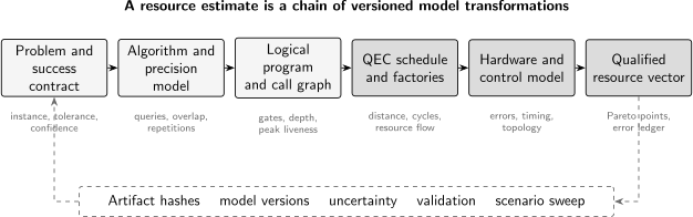
Each arrow is a model transformation with its own version, assumptions, and validation tests. The lower audit loop carries uncertainty and discrepancies back to the layer that produced them.

The intermediate records matter as much as the headline. A useful run emits the symbolic call graph, lowered logical counts, peak liveness trace, scheduled non-Clifford demand, selected code and factory parameters, physical timeline, and a ledger of all approximations.

Logical Counting and Call Graphs

For a hierarchical algorithm, let $m_b(I)$ be the number of calls to subroutine $b$ for instance $I$, and let $c_{b\to g}(\epsilon_b)$ be the cost of lowering that subroutine to primitive $g$ at local tolerance $\epsilon_b$. A symbolic logical count has the form

$$N_g \left( I,\boldsymbol\epsilon \right) = \sum_b m_b(I)\, c_{b\to g}(\epsilon_b).$$

This expression is more informative than a flattened integer. It exposes which subroutine dominates, permits precision sweeps, and allows a new decomposition to replace one term without rebuilding the analysis by hand. Hierarchical tools should also distinguish an analytic cost override from a count obtained by actually decomposing the program.

Counts are not depths

For gate type $g$, keep at least:

• total count $N_g$;
• dependency depth $D_g$;
• maximum simultaneous demand;
• the temporal demand trace when a consumable resource is involved.

A $T$ count determines total magic-state demand under one implementation. A $T$ depth lower-bounds the number of sequential injection layers. Neither by itself determines runtime because factories, routing, Pauli-frame updates, measurements, and classical reactions can stall the schedule. Magic State Distillation defines the factory’s acceptance, delivered-error, throughput, buffering, and correlation contracts; this page composes that model with the workload.

Allocated qubits are not live qubits

Sequential subroutines may reuse ancillas. The relevant peak is

$$Q_{\mathrm{peak}} = \max_t \left[ Q_{\mathrm{data}}(t) +Q_{\mathrm{work}}(t) +Q_{\mathrm{route}}(t) +Q_{\mathrm{factory}}(t) \right],$$

not the sum of every allocation in the source program. A tool therefore needs allocation and deallocation semantics, including whether a released ancilla is known to be in $\lvert0\rangle$, in an arbitrary state, or awaiting reset. Recursive calls and measurement-dependent branches require conservative or branch-weighted liveness rules stated explicitly.

The gate set is part of the result

“One rotation” is not comparable with “thirty $T$ gates.” Counts should name their level:

• source operations;
• high-level arithmetic or oracle calls;
• logical native instructions;
• Clifford+$T$, Clifford+Toffoli, or another fault-tolerant basis;
• physical pulses or measurement rounds.

Gate Decomposition owns exact and approximate synthesis semantics. The estimator should retain the decomposition policy and its precision rather than treating a gate label as a universal unit.

Error and Success Budgets

Error budgeting is not bookkeeping after the estimate. It changes rotation costs, phase-estimation duration, code distances, factory protocols, sampling, and retries.

Keep unlike errors separate

Approximation errors may compose through a norm bound such as

$$\epsilon_{\mathrm{app}} \leq \epsilon_{\mathrm{alg}} +\epsilon_{\mathrm{disc}} +\epsilon_{\mathrm{arith}} +\epsilon_{\mathrm{syn}}.$$

Stochastic failure events may be bounded by

$$\begin{aligned} P_{\mathrm{fail}} \leq{}& P_{\mathrm{logical}} +P_{\mathrm{factory}} +P_{\mathrm{readout}} \\ &+ P_{\mathrm{control}} +P_{\mathrm{post}}. \end{aligned}$$

These equations are examples of two different composition rules. A trace- distance tolerance, an energy bias, an average gate infidelity, and a logical failure probability are not automatically additive. Convert them only through a stated theorem or model.

If $N_R$ synthesized rotations receive local norm tolerances $\epsilon_r$, a simple sufficient rule is

$$\sum_{r=1}^{N_R}\epsilon_r \leq \epsilon_{\mathrm{syn}}.$$

Equal allocation, $\epsilon_r=\epsilon_{\mathrm{syn}}/N_R$, is easy to audit but rarely universally optimal. Since synthesis costs often grow roughly as $\log(1/\epsilon_r)$, a cost-aware allocator can spend more error on expensive or weakly weighted rotations while preserving the global bound.

Success probability multiplies total work

Suppose one complete run succeeds with probability $p_s$, including state preparation, postselection, algorithmic randomness, and verification. The number of independent runs needed for success with confidence at least $1-\delta$ is

$$R_\delta = \left\lceil \frac{\log\delta}{\log(1-p_s)} \right\rceil.$$

The expected number is $1/p_s$, but the expected value does not guarantee a deadline confidence. A complete estimate reports both the one-run resource vector and the repetition policy. If failed attempts are detected early, their average cost should be modeled separately instead of charging every attempt the full runtime.

For sampling an event probability with an additive tolerance $\eta$, a distribution-free Hoeffding bound gives the sufficient shot count

$$N \geq \frac{\log(2/\delta)}{2\eta^2}.$$

Sharper estimators may exploit variance or structure, but the assumed statistical method belongs in the contract.

Fault-Tolerant Lowering

A logical count becomes a physical estimate only after choosing a code, logical instruction set, layout, scheduler, and failure model.

Selecting distance

A common phenomenological fit below threshold is

$$p_{\mathrm L}(d) \approx A \left( \frac{p}{p_{\mathrm{th}}} \right)^{(d+1)/2},$$

where $p$ is a specified physical-noise parameter and $d$ is code distance. The prefactor $A$, threshold $p_{\mathrm{th}}$, exponent, and even the relevant definition of a logical location depend on the code, syndrome circuit, decoder, noise model, and observable. This is not a universal law.

Given $N_{\mathrm{loc}}$ protected locations and a logical-failure allocation $\epsilon_{\mathrm L}$, a conservative selection rule is to choose the smallest supported distance satisfying

$$N_{\mathrm{loc}}\, p_{\mathrm L}(d) \leq \epsilon_{\mathrm L}.$$

The location count depends on the schedule, while the schedule depends on distance-dependent operation time. Distance selection and scheduling may therefore require iteration.

Physical qubits are a system total

An architecture-level count should look schematically like

$$\begin{aligned} Q_{\mathrm{phys}} ={}& Q_{\mathrm{data}} +Q_{\mathrm{workspace}} +Q_{\mathrm{routing}} \\ &+ Q_{\mathrm{factories}} +Q_{\mathrm{control}} +Q_{\mathrm{spares}}. \end{aligned}$$

Multiplying the number of logical data qubits by a patch formula omits temporary ancillas, communication lanes, factories, defective sites, and classical support. Which terms are included must be visible beside the total.

The one-run wall time is likewise a schedule result:

$$T_{\mathrm{run}} = C_{\mathrm L}\tau_{\mathrm L}(d) +T_{\mathrm{feedforward}} +T_{\mathrm{I/O}} +T_{\mathrm{startup}}.$$

Here $C_{\mathrm L}$ is the number of scheduled logical ticks and $\tau_{\mathrm L}(d)$ their architecture-dependent duration. Queueing time is an operational service metric and should not be folded into intrinsic machine runtime unless the claim explicitly asks for time to result.

Factories are a flow constraint

Let a factory produce $m_F$ resource states every $\tau_F$, let the algorithm run for a provisional time $T_{\mathrm{alg}}$, and let total demand be $M$. Ignoring bursts and startup, the average-rate lower bound is

$$F_{\min} \geq \left\lceil \frac{M\tau_F} {m_F T_{\mathrm{alg}}} \right\rceil.$$

Average supply is not sufficient when demand is bursty. If $B_k$ is buffered inventory, $s_k$ supply, $c_k$ consumption, and $B_{\max}$ capacity during tick $k$, then

$$B_{k+1} = \min \left( B_{\max}, B_k+s_k-c_k \right), \qquad B_k\geq0.$$

A stockout stalls the computation unless independent work is available. Extra factories trade qubits and routing capacity for time. Fewer factories can lengthen the computation enough to require a larger code distance, which then changes both data and factory costs.

Routing and classical reaction are resources

Logical operands and resource states must meet under the architecture’s connectivity. Lattice surgery, teleportation, shuttling, photonic links, or modular entanglement each have different area, latency, success, and buffering costs. Adaptive algorithms also impose decoder and feedforward deadlines.

A count-only estimator can provide a lower bound. A physical headline should state whether movement, contention, distillation delivery, decoding, and classical control were scheduled or approximated.

Worked Example: Factory-Constrained Scheduling

Consider a deliberately simplified fault-tolerant scenario, not a hardware forecast. A compiled application has:

$$\begin{aligned} Q&=120 &&\text{live logical data and work qubits},\\ C_{\min}&=8.0\times10^7 &&\text{dependency-limited logical ticks},\\ M&=2.4\times10^8 &&\text{consumed resource states}. \end{aligned}$$

At a selected distance, assume one logical tick takes $\tau_{\mathrm L}=1\,\mu\mathrm{s}$ and one logical qubit occupies $n_{\mathrm L}=1250$ physical qubits. A factory occupies $q_F=5000$ physical qubits and emits one resource state every $\tau_F=10\,\mu\mathrm{s}$.

At the dependency limit,

$$T_{\min} = C_{\min}\tau_{\mathrm L} = 80\,\mathrm{s}.$$

The average-rate factory lower bound is

$$\begin{aligned} F_{\min} &= \left\lceil \frac{ (2.4\times10^8)(10\,\mu\mathrm{s}) }{ 80\,\mathrm{s} } \right\rceil \\ &=30. \end{aligned}$$

Ignoring routing, control, buffers, and spares, the selected point uses

$$\begin{aligned} Q_{\mathrm{data}} &= 120(1250) =150{,}000,\\ Q_{\mathrm{factory}} &= 30(5000) =150{,}000,\\ Q_{\mathrm{subtotal}} &= 300{,}000. \end{aligned}$$

Suppose the chosen code model predicts $p_{\mathrm L}=2.0\times10^{-13}$ per logical-qubit tick. A union-bound estimate for protected data and work is

$$\begin{aligned} P_{\mathrm{logical}} &\leq Q C_{\min}p_{\mathrm L}\\ &= (120)(8.0\times10^7) \times (2.0\times10^{-13})\\ &= 1.92\times10^{-3}. \end{aligned}$$

This fits a hypothetical allocation of $3\times10^{-3}$ before factories, routing, and other failures are added.

Now reduce the machine to ten factories. Producing all states requires at least

$$T_{\mathrm{supply}} = \frac{M\tau_F}{10} = 240\,\mathrm{s},$$

so supply, not circuit dependency, controls the schedule. Keeping the old distance would give

$$P_{\mathrm{logical}} \leq (120)(2.4\times10^8) \times (2.0\times10^{-13}) = 5.76\times10^{-3},$$

which exceeds the same logical allocation. The estimator must select a new distance, update $\tau_{\mathrm L}$ and $n_{\mathrm L}$, reschedule the factories, and test the budget again. The tempting claim “ten factories use 100,000 fewer qubits” is incomplete until this fixed point is recomputed.

Space–Time Tradeoffs and Pareto Frontiers

Resource estimation is naturally multiobjective. A result vector may include

$$\mathbf r = \left( Q_{\mathrm{peak}}, T_{\mathrm{run}}, V_{\mathrm{ST}}, P_{\mathrm{fail}}, B_{\mathrm{classical}}, E_{\mathrm{modeled}} \right),$$

where $V_{\mathrm{ST}}$ is space–time volume, $B_{\mathrm{classical}}$ is a classical bandwidth or memory requirement, and energy appears only when a defensible system model is present.

One configuration dominates another if it is no worse in every declared objective and strictly better in at least one. The non-dominated set is the Pareto frontier. Choosing one point from it requires an external preference: a qubit cap, deadline, power budget, reliability target, or cost function.

When allocation varies in time, a useful physical space–time measure is

$$V_{\mathrm{ST}} = \int_0^{T_{\mathrm{run}}} Q_{\mathrm{active}}(t)\,dt,$$

or its discrete code-cycle analogue. The shortcut $Q_{\mathrm{peak}}T_{\mathrm{run}}$ is an upper bound when resources can be released and reused. Every reported “qubit-hour” should say which convention was used.

Uncertainty and Scenario Analysis

A point estimate with six significant digits can conceal order-of-magnitude model uncertainty. Classify inputs before propagating them:

Input status	Example	Appropriate treatment
exact for the artifact	integer gate count in a hashed circuit	deterministic record
measured	gate time with confidence interval	statistical uncertainty
fitted	logical-error scaling from simulations	fit range and covariance
assumed	independent-noise or perfect-routing model	scenario label
projected	future physical error or yield target	dated sensitivity case

At minimum, publish conservative, reference, and optimistic scenarios without implying that they are calibrated probabilities. When probability distributions are justified, propagate them by sampling the full estimator, including discrete choices such as code distance and factory count.

For a smooth region, the logarithmic sensitivity of output $Y$ to input $x$ is

$$S_{Y,x} = \frac{\partial\log Y}{\partial\log x}.$$

This identifies leverage but can fail at integer boundaries. A small change in physical error may leave an estimate unchanged and then abruptly lower the selected distance by two. Report such transition points and the model branch, not only a local derivative.

Uncertainty also enters through algorithm and compiler choices. Comparing several decompositions, schedulers, and code models is often more informative than placing a narrow confidence interval around one pipeline.

Tool Families and Current Landscape

The following examples were checked against official project documentation on the review date. They illustrate distinct tool families; the list is not a ranking or a completeness claim, and APIs evolve.

Tool family	Current examples	Strongest use	Boundary to inspect
compiler counters	pass statistics in circuit frameworks	concrete counts at a selected IR	count meaning, basis, and liveness may be shallow
hierarchical algorithm models	Qualtran; PennyLane qp.estimator	symbolic decompositions, call graphs, gate and wire costs	analytic overrides and precision policies need validation
domain circuit generators	pyLIQTR	algorithm-derived circuits and Clifford+$T$ analysis, especially Hamiltonian workflows	domain assumptions and imported decompositions
fault-tolerant physical estimators	Microsoft Quantum Resource Estimator; Qualtran physical cost models	code, factory, physical-qubit, runtime, and tradeoff scenarios	built-in architecture and logical-error models
interchange formats	OpenQASM, QIR, QREF	moving programs or resource models between tools	shared syntax does not guarantee shared cost semantics
custom schedulers and system models	research or architecture-specific pipelines	routing, contention, factories, decoders, modules, operations	often least portable and most consequential

The Microsoft Quantum Resource Estimator currently uses a layered application, architecture, error-correction, factory, and error-budget model. Its official documentation lists Q#, Cirq, OpenQASM, QIR, logical counts, and custom applications as inputs and supports comparison of Pareto-optimal qubit–runtime points. A built-in result is still conditional on its selected models.

Qualtran represents algorithms as hierarchical “bloqs.” Its call-graph protocol can use explicit symbolic costs or decompositions, and architecture- independent counts can feed physical cost models. This is valuable for inspectability, but the project explicitly evolves its algorithm library as constructions improve.

pyLIQTR builds circuits from algorithmic workflows and produces Clifford+$T$ resource analyses. PennyLane’s current estimator namespace provides logical resource operators, decomposition controls, wire accounting, and gate counts. QREF aims to provide an open resource-estimation representation. These systems do not make identical promises; compare the exact input level, decomposition leaf set, ancilla semantics, and output schema before comparing numbers.

Choosing and Operating a Tool

Choose the narrowest tool that can answer the declared question while preserving an upgrade path.

Question	Minimum useful capability
Which subroutine dominates asymptotically?	symbolic call graph
What does this concrete logical circuit cost?	semantics-aware counter and liveness analysis
How does rotation precision affect $T$ count?	parameterized synthesis and error allocation
What physical machine fits a deadline?	QEC, factory, routing, timing, and failure models
Which architecture points are non-dominated?	constrained sweep and Pareto analysis
Is a headline reproducible?	versioned artifacts, assumptions, intermediate counts, tests

Before relying on a tool, ask:

1. What object does it accept, and at what abstraction level?
2. Which operations are leaves, and which are decomposed?
3. Are counts symbolic, exact for a concrete artifact, fitted, or heuristic?
4. How are clean and dirty ancillas allocated, released, and reused?
5. Are measurements, resets, branches, and classical reactions represented?
6. Which error metric and composition rule set precision?
7. Are routing, factories, buffers, and decoder latency scheduled?
8. Can hardware, QEC, and factory models be replaced?
9. Does the output include a provenance record and uncertainty ledger?
10. Can small instances be simulated or hand-counted independently?

A calculator that returns physical qubits from only a $T$ count and one error rate may be useful as a rough scenario. It is not an end-to-end architecture estimate unless the missing assumptions are stated and justified.

Reproducibility Record

The publishable object is an estimate bundle, not a screenshot. A machine-readable manifest can use a structure such as:

estimate:
  id: qre-example-2026-08-10
  claim: 'Peak physical qubits and runtime for the declared workload'
  evidence_class: 'model-based estimate'
problem:
  instance: 'versioned input identifier'
  output_tolerance: 1.0e-3
  confidence: 0.99
algorithm:
  name: 'algorithm and construction'
  source_commit: 'commit hash'
  parameters: {}
logical_program:
  ir_format: 'format and version'
  artifact_hash: 'sha256:...'
  gate_set: []
  decomposition_policy: 'named policy'
fault_tolerance:
  code_model: 'name, version, and fit range'
  factory_model: 'name and version'
  error_budget: {}
hardware:
  scenario: 'reference'
  parameters_with_units: {}
scheduler:
  routing_policy: 'named policy'
  feedforward_model: 'named policy'
software:
  packages: {}
  random_seeds: []
outputs:
  logical_counts: {}
  peak_physical_qubits: null
  runtime_seconds: null
  failure_bound: null
uncertainty:
  scenarios: []
  omitted_costs: []

Store the logical artifact, call graph, schedule summary, raw estimator output, plotting code, and environment lockfile beside the manifest. Include units in the data rather than only in a caption. Record warnings, unsupported operations, analytic overrides, cached costs, and any manual arithmetic.

The bundle should make it possible to rerun the original estimate and to swap one layer, such as the hardware model, without reconstructing the algorithm from prose.

Verification and Validation

Resource estimates need tests at several scales.

Subroutine checks

• hand-count identity, swap, add, compare, and controlled variants at small sizes;
• test symbolic formulas against explicit decompositions;
• simulate small circuits to check functional equivalence;
• verify that adjoints and uncomputation return promised ancillas;
• test precision limits and unsupported parameter values.

Accounting checks

• reconcile parent call counts with child totals;
• compare cumulative allocation with peak liveness;
• confirm gate-set labels after every lowering stage;
• check that schedule demand equals reported resource-state consumption;
• check buffer conservation and forbid negative inventory;
• include both branches or state the branch-weighting rule.

Physical-model checks

• reproduce code-distance and factory choices by an independent calculation;
• test fixed-model monotonicity where it should hold;
• verify units and time-scale conversions;
• perturb each major assumption and locate integer transitions;
• compare two tools only after aligning IR, decomposition, error budget, code, physical parameters, and omitted terms.

Cross-tool agreement is evidence only when the contracts match. Disagreement is diagnostically useful: compare intermediate gate counts first, then synthesis, liveness, schedule, distance, factory selection, and physical accounting. Comparing only final qubit totals usually hides the first divergent assumption.

For a published case study, rerun the original artifact at its pinned versions before updating any dependency. Then rerun with current models and report the change as a new estimate. Silent replacement destroys the historical record.

Common Mistakes

• Quoting asymptotic complexity as a machine requirement. Big-$O$ notation suppresses constants and lower layers.
• Calling a source gate count logical. The selected decomposition and precision may change it by orders of magnitude.
• Reporting total allocations as peak qubits. Sequential ancillas can be reused.
• Equating $T$ count with runtime. Dependency depth, factories, routing, and feedforward determine the schedule.
• Using average factory throughput only. Bursty demand can stall despite a favorable average.
• Multiplying logical qubits by one patch formula. Routing, factories, control, defects, and spares are omitted.
• Using one physical infidelity as a circuit failure rate. Error metrics, correlations, leakage, and QEC fits must be modeled consistently.
• Holding code distance fixed while changing runtime. Longer protection can consume the logical-error budget.
• Adding incompatible error quantities. Norm error, estimator bias, infidelity, and failure probability require justified conversions.
• Reporting defaults as facts. Built-in tool parameters are scenarios.
• Publishing only a screenshot or rounded headline. The artifact, versions, inputs, and intermediate records are the reproducible result.
• Treating an estimate as a forecast. A conditional architecture model does not predict when its assumptions will be realized.

Exercises

1. Identify the layer

A paper reports $O(n^3)$ Toffoli gates, another tool reports $4.2\times10^{10}$ logical $T$ gates for $n=2048$, and an architecture model reports $8\times10^6$ physical qubits. Classify the three statements and name one missing contract item for each.

Solution

The first is an asymptotic algorithm or logical-gate estimate; it needs the construction and hidden constants. The second is an instance-level logical estimate; it needs the gate basis, synthesis and decomposition policy, and usually a precision budget. The third is a fault-tolerant physical estimate; it needs at least the logical program, code and distance rule, hardware error and timing model, factories, routing, runtime objective, and failure budget. The numbers cannot be compared as though they were the same resource layer.

2. Peak versus cumulative ancillas

Two sequential subroutines share $40$ data qubits. The first needs $20$ ancillas and the second needs $70$, with all ancillas released cleanly between them. What are the cumulative ancillary allocations and the minimum peak live qubits implied by this information?

Solution

The source may allocate $20+70=90$ ancillary qubits cumulatively, but the ancilla sets can reuse physical storage. The minimum peak is

$$Q_{\mathrm{peak}} = 40+\max(20,70) = 110.$$

This assumes no overlap, no routing ancillas, and immediate reuse after a verified clean release.

3. Allocate synthesis error

A simple norm budget assigns $\epsilon_{\mathrm{syn}}=10^{-3}$ across $N_R=1000$ rotations equally. What local tolerance results? In a toy cost model of $3\log_2(1/\epsilon_r)$ $T$ gates per rotation, estimate the total $T$ count.

Solution

Equal allocation gives

$$\epsilon_r = \frac{10^{-3}}{1000} = 10^{-6}.$$

Since $\log_2(10^6)\simeq19.93$, the toy model gives approximately

$$N_T \simeq 1000(3)(19.93) \simeq 5.98\times10^4.$$

Rounding a synthesis length to an allowed integer sequence would give about $60{,}000$ $T$ gates. The coefficient is part of the toy model, not a universal synthesis law.

4. Select a code distance

Assume the illustrative fit

$$p_{\mathrm L}(d) = 0.1 \left(0.1\right)^{(d+1)/2}.$$

For $N_{\mathrm{loc}}=10^9$ protected locations and logical-failure budget $10^{-3}$, find the smallest odd distance satisfying the union-bound rule.

Solution

The per-location target is

$$p_{\mathrm L} \leq \frac{10^{-3}}{10^9} = 10^{-12}.$$

The model is

$$p_{\mathrm L}(d) = 10^{-(d+3)/2}.$$

Thus $(d+3)/2\geq12$, or $d\geq21$. The smallest allowed odd distance is $d=21$. This answer is conditional on the stated fit and location definition.

5. Count average-rate factories

An application consumes $M=6.0\times10^7$ resource states in $T_{\mathrm{alg}}=30\,\mathrm{s}$. Each factory emits one state every $15\,\mu\mathrm{s}$. What average-rate lower bound follows for the number of factories?

Solution

The bound is

$$\begin{aligned} F_{\min} &= \left\lceil \frac{ (6.0\times10^7)(15\times10^{-6}\,\mathrm{s}) }{ 30\,\mathrm{s} } \right\rceil \\ &= \lceil30\rceil =30. \end{aligned}$$

This does not prove that $30$ factories avoid stalls. Their startup, failure, buffering, delivery routes, and the temporal demand trace remain to be scheduled.

6. Budget repetitions

A complete run has success probability $p_s=0.20$. How many independent runs guarantee at least $99\%$ success under the model? Compare this with the expected number of runs.

Solution

Set $\delta=0.01$:

$$R_{0.01} = \left\lceil \frac{\log(0.01)}{\log(0.8)} \right\rceil = \lceil20.64\ldots\rceil =21.$$

The expected number is only $1/p_s=5$. The expectation and a $99\%$ deadline guarantee answer different questions, so a resource claim should state which one it uses.

7. Find the Pareto frontier

Three estimates satisfy the same failure budget:

Configuration	Physical qubits	Runtime
A	$200{,}000$	$100\,\mathrm{s}$
B	$120{,}000$	$180\,\mathrm{s}$
C	$250{,}000$	$150\,\mathrm{s}$

Which configurations are Pareto optimal with respect to fewer qubits and shorter time?

Solution

A and B are non-dominated: A is faster, while B uses fewer qubits. C is dominated by A because A uses both fewer qubits and less time. Choosing between A and B requires an external qubit cap, deadline, or cost function.

8. Diagnose a cross-tool disagreement

Two tools receive circuits described as “the same algorithm.” One reports twice the $T$ count and half the logical qubits of the other. Give a useful diagnostic order.

Solution

First compare instance and precision parameters, then the input IR and qubit ordering. Align the decomposition leaf set, rotation-synthesis rule, arithmetic construction, controlled and adjoint variants, and clean-versus-dirty ancilla policy. Compare hierarchical subroutine counts before flattened totals. Next inspect ancilla liveness and uncomputation.

Only after the logical artifacts agree should one compare QEC, scheduling, factories, and physical assumptions. The observed tradeoff may be legitimate: one construction can spend extra $T$ gates to save workspace.

9. Audit a headline estimate

A chart states that a useful application needs “one million qubits and one day.” List the minimum evidence needed before treating it as a decision-grade estimate.

Solution

Require the exact problem instance and success criterion; algorithm and input- access model; approximation and confidence budgets; logical program or symbolic call graph; gate set, counts, depth, measurements, and peak liveness; compiler and synthesis versions; QEC code, logical ISA, distance and decoder model; physical error and timing parameters with provenance; factory, routing, buffer, feedforward, yield, and retry assumptions; total failure accounting; uncertainty or scenario sweeps; intermediate outputs and validation tests; and the complete software environment or estimator manifest.

Finally determine whether “qubits” means logical or physical and whether “one day” is one-run intrinsic runtime, expected time to success, a confidence deadline, or time including queue and classical processing.

Research Status

Hierarchical gate counting, reversible-circuit analysis, surface-code space–time models, magic-state distillation accounting, and layered resource estimation are established methods. Tool support for symbolic costs, intermediate representations, physical scenarios, and Pareto exploration is substantial.

The field remains active because every layer is improving. Algorithmic constructions, rotation synthesis, arithmetic, error correction, lattice surgery, magic-state cultivation, biased-noise codes, modular architectures, decoder hardware, and physical platforms can each move a headline estimate by large factors. Interoperable resource formats and common benchmark suites are still developing.

Consequently, a resource estimate should be read as a versioned engineering model. Its most durable contribution is often the transparent pipeline and sensitivity map, not the final integer.

Further Connections

• Resource Estimation defines the logical, encoded, physical, timing, factory, error-budget, and spacetime quantities that estimation tools compute.
• Quantum Software Stack places estimation beside source programs, compilers, target models, runtime services, and provenance records.
• Circuit Intermediate Representations defines typed operations, capabilities, semantics, and pass history at the boundaries an estimator consumes.
• Gate Decomposition owns exact and approximate synthesis, gate-set changes, phase conventions, and local precision.
• Circuit Optimization develops semantics-preserving transformations and evidence for improvements in count, depth, liveness, and hardware-weighted cost.
• Surface Code develops the code geometry, repeated checks, logical operations, threshold contract, and architecture-level overhead used by many physical estimates.
• Threshold Theorem explains when recursive or distance-based suppression exists, how its overhead scales, and why a theorem threshold is not a universal estimator input.
• Lattice Surgery supplies the protected parity primitives, spacetime scheduling constraints, routing assumptions, and patch costs that a surface-code estimator must model.
• Metrics for Quantum Hardware defines the measured error, time, leakage, crosstalk, throughput, and logical metrics supplied to hardware scenarios.
• Algorithmic Benchmarking distinguishes measured algorithm execution from conditional fault-tolerant projections and supplies the task, acceptance, retry, and end-to-end cost boundary an estimate must preserve.
• Reporting Standards supplies the resource-estimate profile, manifest, provenance, scenario-uncertainty, artifact-version, and correction requirements for a published projection.
• Shor Algorithm provides a canonical example of how arithmetic, retries, logical resources, factories, code assumptions, and runtime tradeoffs change a cryptographic estimate.
• Quantum Phase Estimation connects precision, coherent evolution time, overlap, repetition, and application-level resource costs.
• Qubitization and Quantum Signal Processing supplies a concrete oracle-to-logical-gate ledger for block-encoded Hamiltonian simulation and spectral readout.
• Simulation of Quantum Chemistry supplies the molecular-model, encoding, state-preparation, eigensolver, measurement, and validation inputs that a chemistry resource estimate must preserve.
• Simulation of Quantum Materials supplies the cell, boundary, representation, state, observable, finite-size, workflow-multiplicity, and validation inputs that a materials estimate must preserve.
• Variational Quantum Algorithms accounts for objective, gradient, metric, adaptive-shot, optimizer, seed, and fresh-validation costs that a shallow-circuit headline can omit.
• VQE gives the energy-estimation, grouping, mitigation, restart, and validation ledger for a concrete hybrid eigensolver.
• Quantum Chemistry Case Studies compares executed small-molecule workflows with FeMoco, catalysis, and P450 fault-tolerant estimates under explicit chemistry-model boundaries.
• Negative Results and Limitations separates proved lower bounds from present-day overhead bottlenecks and identifies the assumptions that could change an estimate.
• Claims, Hype, and Evidence Standards gives the evidence contract for publishing estimates without turning assumptions into forecasts.

References

1. M. E. Beverland et al., “Assessing requirements to scale to practical quantum advantage,” arXiv:2211.07629 (2022), arXiv:2211.07629.
2. A. G. Fowler, M. Mariantoni, J. M. Martinis, and A. N. Cleland, “Surface codes: Towards practical large-scale quantum computation,” Physical Review A 86, 032324 (2012), doi:10.1103/PhysRevA.86.032324.
3. D. Litinski, “A game of surface codes: Large-scale quantum computing with lattice surgery,” Quantum 3, 128 (2019), doi:10.22331/q-2019-03-05-128.
4. C. Gidney and A. G. Fowler, “Efficient magic state factories with a catalyzed $|CCZ\rangle$ to $2|T\rangle$ transformation,” Quantum 3, 135 (2019), doi:10.22331/q-2019-04-30-135.
5. C. Gidney and M. Ekerå, “How to factor 2048 bit RSA integers in 8 hours using 20 million noisy qubits,” Quantum 5, 433 (2021), doi:10.22331/q-2021-04-15-433.
6. M. Reiher, N. Wiebe, K. M. Svore, D. Wecker, and M. Troyer, “Elucidating reaction mechanisms on quantum computers,” Proceedings of the National Academy of Sciences 114, 7555–7560 (2017), doi:10.1073/pnas.1619152114.
7. V. von Burg et al., “Quantum computing enhanced computational catalysis,” Physical Review Research 3, 033055 (2021), doi:10.1103/PhysRevResearch.3.033055.
8. N. J. Ross and P. Selinger, “Optimal ancilla-free Clifford+$T$ approximation of $z$-rotations,” Quantum Information and Computation 16, 901–953 (2016), arXiv:1403.2975.
9. M. P. Harrigan et al., “Expressing and analyzing quantum algorithms with Qualtran,” arXiv:2409.04643 (2024), arXiv:2409.04643.
10. Microsoft, “Introduction to the resource estimator,” Microsoft Learn, reviewed 2026-08-10, official documentation.
11. Google Quantum AI, “Qualtran,” and the Qualtran project, “The call graph protocol,” reviewed 2026-08-10, project overview, official documentation.
12. MIT Lincoln Laboratory and USC Information Sciences Institute, “pyLIQTR documentation,” reviewed 2026-08-10, official documentation.
13. PennyLane, “Quantum resource estimation,” reviewed 2026-08-10, official documentation.
14. PsiQuantum, “Quantum Resource Estimation Format,” reviewed 2026-08-10, official documentation.
15. A. W. Cross et al., “OpenQASM 3: A broader and deeper quantum assembly language,” ACM Transactions on Quantum Computing 3, article 12 (2022), doi:10.1145/3505636.
16. M. A. Nielsen and I. L. Chuang, Quantum Computation and Quantum Information, 10th anniversary ed., Cambridge University Press (2010), doi:10.1017/CBO9780511976667.