Simulation of Quantum Chemistry

Short Definition

Quantum simulation of chemistry is the end-to-end task of converting a declared molecular model into a finite fermionic or first-quantized operator, encoding that operator and its target state on a quantum processor, applying an eigensolver or dynamics algorithm, and translating measured data into a chemically defined quantity with an explicit uncertainty and resource ledger.

The phrase does not identify one algorithm. A chemistry workflow may use a variational eigensolver, phase estimation, qubitization, product formulas, real-time response, imaginary-time-inspired state preparation, or a quantum impurity solver embedded in a larger classical calculation. These routes consume different input interfaces and return different outputs.

Nor does a quantum processor remove chemical modeling choices. Geometry, nuclear treatment, relativistic terms, environment, one-particle basis, frozen core, active space, integral approximation, charge, spin, and state identity are fixed before a gate is applied. A circuit can solve its encoded Hamiltonian accurately while that Hamiltonian remains inadequate for the scientific question.

Canonical Scope

This page is the canonical home for the molecule-to-processor workflow:

• defining the chemical target and finite electronic model;
• translating one- and two-electron integrals into an executable operator;
• choosing second- or first-quantized representations;
• mapping fermionic modes to qubits and reducing exact symmetry sectors;
• connecting state preparation to VQE, phase estimation, dynamics, and response calculations;
• tracking factorization, simulation, synthesis, hardware, and sampling errors alongside basis and active-space errors;
• expanding orbital counts into queries, gates, qubits, shots, and physical resources;
• validating the encoded spectrum and the final chemical claim.

Molecular Hamiltonian owns the full electron–nuclear Coulomb operator and its reductions. Electronic Structure Overview owns basis sets, correlation models, and molecular method selection. Many-Particle Hamiltonians owns the general second-quantized operator derivation. VQE, Quantum Phase Estimation, and Qubitization and Quantum Signal Processing own their respective algorithmic guarantees. Quantum Chemistry Case Studies owns the evidence-centered comparison of experiments and resource estimates. Quantum Algorithms for Chemistry and Materials owns the compact cross-algorithm selection bridge after this page has fixed the molecular model and encoded task; this page retains the molecule-to-processor workflow and chemical validation.

The Computational Contract

A reproducible chemistry task begins with a specification such as

$$\mathfrak C = \left( \mathcal G, \hat H_{\mathrm{phys}}, \mathcal B, \mathcal A, \Gamma, \rho_{\mathrm{in}}, \mathcal O, \epsilon, \delta \right).$$

Here:

Symbol	Meaning	Representative choice
$\mathcal G$	geometry and nuclear data	fixed equilibrium geometry or reaction coordinate
$\hat H_{\mathrm{phys}}$	physical Hamiltonian model	nonrelativistic clamped nuclei with a named pseudopotential
$\mathcal B$	one-particle representation	Gaussian orbitals, plane waves, grid, or localized orbitals
$\mathcal A$	retained correlated space	all orbitals, frozen core, or a declared active space
$\Gamma$	target sector and state identity	electron number, spin, point-group irrep, and root
$\rho_{\mathrm{in}}$	prepared input	Hartree–Fock determinant or multireference trial state
$\mathcal O$	requested output	energy difference, density, force, spectrum, or correlation function
$\epsilon$	accepted numerical and model error	property-specific tolerance with an allocation by source
$\delta$	failure probability	confidence requirement for the complete workflow

The output contract matters as much as the Hamiltonian. Estimating one eigenvalue is not the same task as preparing its eigenstate. Preparing a state does not reveal all of its amplitudes. A reaction barrier requires several geometries and consistent state tracking. A force requires a derivative protocol and response terms, not only a total energy at one point.

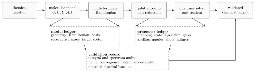
A quantum chemistry calculation is a chain of typed interfaces. The model ledger fixes what physical problem is encoded; the processor ledger records how it is represented and solved. Validation must reach back across both ledgers before a circuit result becomes a chemical claim.

From Molecular Model to Finite Hamiltonian

Fixed-geometry electronic problem

For a standard nonrelativistic, field-free, clamped-nuclei calculation in atomic units, the electronic Hamiltonian is

$$\begin{aligned} \hat H_{\mathrm e}(\mathbf R) ={}& -\frac12\sum_i\nabla_i^2 -\sum_{iA}\frac{Z_A}{r_{iA}} +\sum_{i<j}\frac{1}{r_{ij}} \\ &+ E_{\mathrm{NN}}(\mathbf R). \end{aligned}$$

This equation already encodes assumptions. The nuclei are parameters rather than quantum degrees of freedom, the interaction is instantaneous Coulomb, and relativistic, radiative, solvent, and external-field effects are absent unless added deliberately. The scalar nuclear repulsion $E_{\mathrm{NN}}$ may be stored inside the qubit Hamiltonian or restored classically. The convention must remain consistent when comparing geometries.

Choose $N$ orthonormal spin-orbitals $\{\phi_p\}$. With antisymmetrized two-electron integrals, the finite operator is

$$\begin{aligned} H_{\mathrm{orb}} ={}& E_{\mathrm{NN}} +\sum_{pq}h_{pq}a_p^\dagger a_q \\ &+ \frac14\sum_{pqrs} \langle pq\Vert rs\rangle a_p^\dagger a_q^\dagger a_s a_r. \end{aligned}$$

The finite Fock space has dimension $2^N$, while a fixed $\eta$-electron sector has dimension

$$\dim\mathcal H_{N,\eta} = \binom{N}{\eta}.$$

Quantum storage can represent amplitudes in this sector compactly, but that fact alone gives neither an efficient state-preparation algorithm nor an efficient route to every observable.

Integral conventions must be executable

Chemistry software also commonly exports unantisymmetrized two-electron integrals and writes

$$H_2 = \frac12 \sum_{pqrs} \langle pq\vert rs\rangle a_p^\dagger a_q^\dagger a_s a_r.$$

This is equivalent to the $1/4$ expression only when the integral definition, index order, spin convention, and antisymmetrization are matched. Spatial- orbital integrals with implicit spin labels are not the same data tensor as spin-orbital integrals. Before mapping to qubits, an implementation should test:

• Hermiticity of the one-body matrix;
• permutation and conjugation symmetries of the two-body tensor;
• agreement between direct matrix elements and the assembled Fock-space operator on a small sector;
• whether nuclear repulsion and frozen-core constants are included;
• the units and orbital ordering used by every file boundary.

A factor-of-two or index-permutation error can preserve a superficially reasonable spectrum while changing the chemistry.

Frozen cores and active spaces

If a set $C$ of spin-orbitals is constrained to remain occupied, normal ordering with respect to that determinant gives an active-space Hamiltonian

$$\begin{aligned} H_{\mathrm{act}} ={}&E_{\mathrm{core}} +\sum_{p,q\in A} h^{\mathrm{eff}}_{pq}a_p^\dagger a_q \\ &+ \frac14 \sum_{p,q,r,s\in A} \langle pq\Vert rs\rangle a_p^\dagger a_q^\dagger a_s a_r, \end{aligned}$$

where, for occupied spin-orbitals $i,j\in C$,

$$E_{\mathrm{core}} = E_{\mathrm{NN}} +\sum_{i\in C}h_{ii} +\frac12\sum_{i,j\in C} \langle ij\Vert ij\rangle,$$

and

$$h^{\mathrm{eff}}_{pq} = h_{pq} +\sum_{i\in C} \langle pi\Vert qi\rangle.$$

The active indices $p,q,r,s$ run only over $A$. This reduction is exact for the constrained frozen-core model, not for the original molecular Hamiltonian. Orbitals excluded from $A$ cannot acquire arbitrary correlated occupations. An active space must therefore be justified by occupations, entanglement or orbital diagnostics, state character, convergence tests, and the property being predicted.

Changing geometry can change which orbitals are chemically important. Potential-energy curves and reaction paths require a consistent orbital and state-tracking protocol; independently choosing the easiest active space at each point can manufacture discontinuities or favorable error cancellation.

Representation Choices

Second quantization

In an occupation encoding, one qubit records whether each spin-orbital is empty or occupied. Before exact symmetry reduction, $N$ spin-orbitals require $N$ qubits even when only $\eta\ll N$ electrons are present. The computational basis state

$$\lvert n_0n_1\cdots n_{N-1}\rangle, \qquad n_p\in\{0,1\},$$

represents a Slater determinant with the declared fermionic mode order. Second quantization makes determinant preparation and number-conserving excitation operators natural, and it is the standard language for many molecular-orbital algorithms.

First quantization

A first-quantized encoding stores the orbital or grid label of each of the $\eta$ electrons. A compact orbital encoding can use approximately

$$\eta\left\lceil\log_2N\right\rceil$$

data qubits before ancillas. The register must nevertheless represent an antisymmetric state and implement kinetic, potential, permutation, and data- access operations coherently. Plane-wave and real-space structures can make these operations favorable; arbitrary molecular-orbital problems may favor second quantization instead.

Question	Second quantization	First quantization
stored labels	one occupation bit per mode	one orbital or grid label per electron
data-qubit scale	$N$	roughly $\eta\log_2N$
antisymmetry	encoded by operator algebra and mode mapping	must be built into the state or algorithm
natural inputs	molecular orbitals and fermionic excitations	plane waves, grids, compact particle registers
common bottleneck	Pauli strings, measurements, PREPARE/SELECT	antisymmetric preparation, arithmetic, interaction oracles

The smaller data register is not automatically the cheaper algorithm. Ancillas, arithmetic width, oracle depth, normalization, state preparation, and fault-tolerant non-Clifford cost decide the comparison.

Fermions on Qubits

Jordan–Wigner convention

Using the site-wide convention that $\lvert0\rangle$ is empty and $\lvert1\rangle$ is occupied, the Jordan–Wigner map is

$$\begin{aligned} a_p &= \left(\prod_{j<p}Z_j\right) \frac{X_p+iY_p}{2}, \\ a_p^\dagger &= \left(\prod_{j<p}Z_j\right) \frac{X_p-iY_p}{2}. \end{aligned}$$

Consequently,

$$n_p = a_p^\dagger a_p = \frac{I-Z_p}{2}.$$

The $Z$ string records the parity of earlier modes and enforces the anticommutation relations. Jordan–Wigner Transformation owns the full proof and the consequences of changing the mode order.

After substitution and collection, the molecular Hamiltonian becomes

$$H_q = c_0I + \sum_{\ell=1}^{L}c_\ell P_\ell,$$

where each $P_\ell$ is a tensor product of Pauli operators. A dense generic two-body tensor has $O(N^4)$ entries, but integral symmetry, locality, screening, low-rank structure, and exact collection can materially change the number and cost of distinct Pauli terms.

Bravyi–Kitaev and parity encodings distribute occupation and parity information differently. They can shorten some strings or expose useful symmetries, but they do not change the spectrum of the correctly encoded fermionic operator. A benchmark must compare compiled circuits under the same mode order, hardware graph, state preparation, and observable protocol.

Exact symmetry reduction

The electronic Hamiltonian usually commutes with particle number, $S_z$, and selected spatial or discrete symmetries. In a qubit representation, suppose independent Pauli symmetries $S_j$ satisfy

$$[H_q,S_j]=0, \qquad S_j\lvert\psi\rangle=s_j\lvert\psi\rangle, \qquad s_j\in\{+1,-1\}.$$

A Clifford change of basis can map each $S_j$ to a single-qubit $Z$ operator. Fixing its known eigenvalue then removes that qubit from the target block. This tapering is exact only for the selected sector. The state-preparation circuit, observables, and every geometry in a comparison must use compatible symmetry labels.

A penalty such as

$$H_{\mu} = H_q + \mu \left( \hat N-\eta \right)^2$$

is different. It discourages the wrong particle-number sector but does not remove it exactly, and it can enlarge coefficient norms, measurement variance, or simulation normalization. Symmetry-preserving ansatzes and exact tapering are preferable when their assumptions hold.

Total spin deserves separate attention. Fixing $N_\alpha-N_\beta$ fixes $S_z$, not $S^2$. A trial state may therefore contain unwanted total-spin components even while particle number and spin projection are correct.

State Preparation Is Part of the Algorithm

A Hartree–Fock determinant maps to a computational-basis bitstring and is usually inexpensive to prepare after the orbital basis is fixed. Its overlap with a target eigenstate,

$$p_0 = \left| \langle E_0\vert\psi_{\mathrm{in}}\rangle \right|^2,$$

can nevertheless be poor for bond breaking, open shells, transition-metal complexes, conical intersections, and other multireference regimes.

If an ideal spectral algorithm samples the desired eigenvalue with probability $p_0$, the chance of seeing it at least once in $r$ independent runs is

$$1-(1-p_0)^r.$$

Reaching success probability at least $1-\delta$ requires

$$r \geq \frac{\log\delta}{\log(1-p_0)}.$$

For small $p_0$, this scales approximately as $\log(1/\delta)/p_0$. State preparation can therefore erase a favorable Hamiltonian-simulation query count.

Correlated inputs include short configuration-interaction expansions, multiconfigurational states, adiabatically prepared states, tensor-network states compiled into circuits, or states produced by a variational routine. Their classical preprocessing, amplitude loading, normalization, circuit depth, and certification all belong in the resource ledger. Quoting the cost of phase estimation while assuming an uncosted exact eigenstate is not an end-to-end estimate.

Choosing the Quantum Route

Variational energy estimation

For a parameterized state $\lvert\psi(\boldsymbol\theta)\rangle$, VQE estimates

$$E(\boldsymbol\theta) = c_0 + \sum_{\ell=1}^{L} c_\ell \langle P_\ell\rangle_{\boldsymbol\theta}$$

and uses a classical optimizer to reduce it. This replaces long coherent evolution with many state preparations, measurements, and adaptive quantum–classical iterations. The variational principle is rigorous for the ideal expectation of a normalized state, but finite sampling, optimizer selection, noise mitigation, and postselection alter the statistical claim.

If Pauli terms are measured independently with $m_\ell$ shots, their contribution to the estimator variance is

$$\operatorname{Var}(\widehat E) = \sum_\ell \frac{c_\ell^2v_\ell}{m_\ell}, \qquad v_\ell = \operatorname{Var}(P_\ell).$$

For fixed target variance $\epsilon_{\mathrm{stat}}^2$, the ideal continuous shot allocation obeys

$$m_\ell \propto |c_\ell|\sqrt{v_\ell},$$

with total

$$M_{\min} = \frac{ \left( \sum_\ell |c_\ell|\sqrt{v_\ell} \right)^2 }{ \epsilon_{\mathrm{stat}}^2 }.$$

Commuting-group measurements, basis rotations, low-rank measurement schemes, classical shadows, and covariance-aware allocation can change this ledger. Counting groups alone is insufficient: groups have different circuit depths, variances, covariances, and shot allocations. The VQE page owns ansatz design, optimization, variational error, mitigation, and independent validation.

Phase estimation of molecular energies

Let

$$U(t_0) = \exp\!\left[ -\frac{i}{\hbar} \left(H_q-E_{\mathrm{ref}}I\right)t_0 \right].$$

For an eigenstate $\lvert E_k\rangle$,

$$U(t_0)\lvert E_k\rangle = e^{-i(E_k-E_{\mathrm{ref}})t_0/\hbar} \lvert E_k\rangle.$$

Phase estimation resolves this phase modulo $2\pi$. If the allowed energy window is closed and has width $W$, choosing

$$t_0 < \frac{2\pi\hbar}{W}$$

keeps the phase map injective within that window after the offset convention is fixed. Equality is usable for a half-open interval with a fixed endpoint convention; practical implementations usually leave a guard margin. With $m$ binary phase bits, the grid scale in energy is approximately

$$\Delta E_{\mathrm{grid}} \sim \frac{2\pi\hbar}{2^m t_0}.$$

The longest controlled evolution and total interrogation time grow as $O(2^m t_0)$, hence as $O(\hbar/\Delta E)$ up to algorithm- and confidence- dependent factors. Reporting only the number of phase ancillas hides this coherent-time cost.

The output is a spectral sample weighted by the input overlaps. Phase estimation does not create the ground state from an arbitrary trial state, and it does not by itself identify which sampled root has the desired chemical character. Quantum Phase Estimation owns the exact finite-bit distribution, confidence amplification, iterative variants, Fourier conventions, and total controlled-power accounting.

Product formulas, LCU, and qubitization

Phase estimation requires controlled access to molecular time evolution or a related signal unitary. The implementation can use:

Method family	Chemistry-facing input	Important chemistry-dependent cost
Trotter–Suzuki	exponentials of fermionic or Pauli terms	ordering, commutators, basis rotations, routed Pauli strings
truncated Taylor or LCU	coefficient preparation and SELECT	coefficient one-norm, state preparation, amplification, arithmetic
qubitization and QSP	controlled block encoding and inverse	normalization $\alpha$, PREPARE/SELECT, phase synthesis, work registers
interaction picture	a split $H=A+B$ with one easy part	cost of the easy frame and integrated norm of the residual interaction

For an LCU decomposition

$$H_q = \sum_j w_jU_j,$$

a direct block encoding often has normalization

$$\lambda = \sum_j|w_j|.$$

The qubitized time parameter is $\lambda|t|/\hbar$, not merely $\|H_q\||t|/\hbar$. Orbital rotations, integral factorization, energy shifts, and decomposition strategy can change both $\lambda$ and the gate cost of one PREPARE/SELECT query. Hamiltonian Simulation owns method comparison, while Trotter–Suzuki Methods and Qubitization and Quantum Signal Processing own the executable constructions.

Dynamics and response

Chemistry is not only a ground-energy problem. Real-time simulation can target

$$C_{AB}(t) = \langle\psi_0\vert A(t)B(0) \vert\psi_0\rangle,$$

transition amplitudes, dipole response, charge migration, scattering, or nonadiabatic dynamics in an enlarged model. A frequency-domain spectrum may require a windowed transform of many time samples, so maximum evolution time, time spacing, window bias, and shot noise jointly set spectral resolution.

Forces, reduced density matrices, and response properties require additional observables. The Hellmann–Feynman term alone may be insufficient when the basis, orbitals, or variational parameters depend on geometry. Pulay and response contributions must be included according to the chosen electronic- structure model.

Factorization and Data Access

The two-electron tensor is structured. A generic low-rank representation can write its induced operator schematically as

$$H_2 \approx H_{1,\mathrm{corr}} + \frac12 \sum_{\ell=1}^{R} \left( \sum_{pq} W_{pq}^{(\ell)}a_p^\dagger a_q \right)^2,$$

where $H_{1,\mathrm{corr}}$ contains the one-body correction required by reordering. Diagonalizing each matrix $W^{(\ell)}$ turns a dense collection of quartic terms into orbital rotations and diagonal number interactions. Double factorization refines this structure by truncating eigencomponents within each factor.

Tensor hypercontraction uses a different approximation, schematically

$$(pq\vert rs) \approx \sum_{\mu\nu} X_{p\mu}X_{q\mu} Z_{\mu\nu} X_{r\nu}X_{s\nu},$$

for a real-orbital convention. Such factorizations can reduce storage, measurement settings, basis-rotation cost, or block-encoding complexity. They also introduce a threshold-dependent operator error. The report must include:

• the factorization family and rank-selection rule;
• the norm or observable used to certify truncation;
• coefficient precision and data-layout assumptions;
• the resulting Pauli count or block-encoding normalization;
• PREPARE, SELECT, QROM, arithmetic, and basis-rotation costs;
• validation against the unfactorized finite Hamiltonian on tractable cases.

An asymptotically compact tensor is not useful if loading its factors dominates the calculation. Conversely, treating every two-electron integral as an unstructured independent Pauli term can miss the principal source of modern resource reductions.

Worked Example: Minimal Hydrogen as an Encoding Audit

Consider $\mathrm H_2$ in a minimal spatial basis. Bonding and antibonding orbitals each carry two spin states, so the second-quantized model has four spin-orbitals. A direct occupation encoding therefore begins with four qubits, not two electrons’ worth of qubits.

Order the spin-orbitals as

$$g\alpha, \quad g\beta, \quad u\alpha, \quad u\beta.$$

In the two-electron, $M_S=0$, even spatial-symmetry singlet block, the paired determinants

$$\lvert g^2\rangle = \lvert1100\rangle, \qquad \lvert u^2\rangle = \lvert0011\rangle$$

span a two-dimensional invariant subspace for this minimal model. In that basis, write

$$H_{\mathrm{sub}} = \begin{pmatrix} A & B\\ B & D \end{pmatrix},$$

where real orbitals have been chosen. Identifying $\lvert g^2\rangle\leftrightarrow\lvert0_L\rangle$ and $\lvert u^2\rangle\leftrightarrow\lvert1_L\rangle$ gives

$$H_{\mathrm{sub}} = c_0I+c_xX+c_zZ,$$

with

$$c_0 = \frac{A+D}{2}, \qquad c_x=B, \qquad c_z = \frac{A-D}{2}.$$

The two eigenvalues are

$$E_\pm = c_0 \pm \sqrt{c_x^2+c_z^2}.$$

This reduction is an excellent audit case: construct the four-qubit Hamiltonian, project it into the declared symmetry block, and verify the same $E_\pm$ from the logical one-qubit form. It does not establish that a chemically converged hydrogen calculation generally needs one qubit. The result relies on a minimal basis, fixed particle number, selected spin and spatial symmetry, and a two-dimensional invariant block. Enlarging the basis or changing the target state changes the model.

The Layered Error Ledger

Let $E_{\mathrm{phys}}$ be the desired value for the intended physical system. Introduce a chain of exact values for successive approximations:

$$\begin{aligned} E_{\mathrm{phys}} &\longrightarrow E_{\mathrm{Ham}} \longrightarrow E_{\mathrm{basis}} \longrightarrow E_{\mathrm{act}} \\ &\longrightarrow E_{\mathrm{data}} \longrightarrow E_{\mathrm{alg}} \longrightarrow \widehat E. \end{aligned}$$

The difference telescopes exactly:

$$\begin{aligned} \widehat E-E_{\mathrm{phys}} ={}& (\widehat E-E_{\mathrm{alg}}) +(E_{\mathrm{alg}}-E_{\mathrm{data}}) \\ &+(E_{\mathrm{data}}-E_{\mathrm{act}}) +(E_{\mathrm{act}}-E_{\mathrm{basis}}) \\ &+(E_{\mathrm{basis}}-E_{\mathrm{Ham}}) +(E_{\mathrm{Ham}}-E_{\mathrm{phys}}). \end{aligned}$$

These terms can represent:

Difference	Representative sources
$E_{\mathrm{Ham}}-E_{\mathrm{phys}}$	nuclear model, relativity, environment, omitted interactions
$E_{\mathrm{basis}}-E_{\mathrm{Ham}}$	finite orbital or grid representation
$E_{\mathrm{act}}-E_{\mathrm{basis}}$	frozen core, active-space restriction, embedding
$E_{\mathrm{data}}-E_{\mathrm{act}}$	integral rounding, screening, low-rank factorization
$E_{\mathrm{alg}}-E_{\mathrm{data}}$	ansatz, optimization, finite-time simulation, phase resolution
$\widehat E-E_{\mathrm{alg}}$	synthesis, hardware, sampling, readout, mitigation, selection bias

The labels are diagnostic, not a promise that each component can be measured independently. Errors may correlate or cancel, and nonlinear mitigation can invalidate a naive probabilistic interpretation. The triangle inequality still supplies a conservative allocation when certified bounds are available.

The conventional $1\,\mathrm{kcal\,mol^{-1}}$ chemical-accuracy scale is approximately $1.5936\times10^{-3}E_{\mathrm h}$, but it is not a universal success criterion. Spectroscopic splittings, barrier heights, spin gaps, forces, and response properties have different tolerances. Sub-millihartree agreement with exact diagonalization of an inadequate active-space Hamiltonian is an algorithmic result, not automatically chemical accuracy.

For an energy difference

$$\Delta E = E_B-E_A,$$

consistent Hamiltonians, bases, active spaces, state identities, and statistical protocols are essential. Correlated errors may cancel; separately optimized approximations may not. Report uncertainty and covariance for the difference itself rather than adding two favorable absolute-error summaries.

Resource Accounting

An orbital count is only the first line of a resource estimate.

Logical resources

A second-quantized estimate should state:

• spin-orbital count and qubits before reduction;
• every frozen orbital, active electron, and active orbital;
• symmetry generators, chosen eigenvalues, and qubits tapered;
• state-preparation gates and success or overlap assumptions;
• Pauli terms or block-encoding normalization;
• logical Clifford, arbitrary rotation, Toffoli or $T$ counts;
• logical depth, connectivity assumptions, clean and dirty ancillas;
• controlled-operation overhead for phase estimation;
• measurement settings, state preparations, optimizer calls, and retries.

For qubitized phase estimation, a useful schematic is

$$C_{\mathrm{logical}} \sim N_{\mathrm{query}} C_{\mathrm{query}} +C_{\mathrm{state}} +C_{\mathrm{phase}} +C_{\mathrm{readout}},$$

where $C_{\mathrm{query}}$ expands PREPARE, SELECT, their inverses, reflection, controls, QROM, and arithmetic. A theorem-level query count with $C_{\mathrm{query}}=1$ is not a gate estimate.

For VQE, a corresponding wall-clock schematic is

$$T_{\mathrm{VQE}} \sim \sum_{k=1}^{N_{\mathrm{eval}}} \sum_{g=1}^{N_{\mathrm{groups}}} m_{kg} \left( t_{\mathrm{prepare},k} +t_{\mathrm{basis},g} +t_{\mathrm{readout}} \right),$$

plus compilation, queueing, calibration, classical optimization, and validation. Circuit depth and shot throughput can trade against one another.

Physical resources

Fault-tolerant projections must further declare the code, physical error model, cycle time, code distance, logical failure allocation, magic-state factories, routing, measurement latency, parallelism, physical qubits, and runtime. Those quantities are conditional engineering outputs, not delivery dates. Resource Estimation Tools owns the reproducible logical-to-physical workflow.

Classical work remains

The quantum stage commonly depends on classical geometry generation, orbital optimization, integral evaluation, localization, active-space selection, factorization, circuit generation, phase finding, decoding, optimization, and validation. A fair comparison counts the complete workflow on both sides and uses the strongest applicable classical baseline for the same Hamiltonian and observable.

Validation Strategy

Validation should proceed from the smallest interface outward.

Model and integral checks

1. Record geometry, charge, multiplicity, Hamiltonian, basis, frozen core, active space, orbital order, units, and constant-energy convention.
2. Check one- and two-electron tensor symmetries and particle-number conservation.
3. Compare active-space integrals and energies against an independent implementation or archived reference artifact.
4. Converge basis, active space, factorization threshold, and geometry for the requested property rather than only for one total energy.

Encoding checks

1. Build the fermionic matrix and qubit matrix for a tractable instance and compare spectra in the same symmetry sector.
2. Verify occupation, parity, and mode-order conventions on basis states.
3. Check every tapered symmetry eigenvalue and reconstruct selected observables before trusting the reduced circuit.
4. Confirm that coefficient rounding and factorization satisfy the declared operator or observable tolerance.

Algorithm and output checks

1. Compare noiseless circuits with exact diagonalization at small sizes.
2. Test limiting cases: vanishing interaction, separated fragments, known symmetries, and conserved quantities.
3. Refine Trotter steps, QSP degree, phase bits, shots, and optimizer budgets independently.
4. Validate a selected variational state with fresh measurements rather than the data used to select it.
5. Track state identity across geometries using overlaps, densities, symmetries, and transition properties.
6. Compare the final observable with a matched classical method and report where the comparison is exact, approximate, or unavailable.

Agreement with exact diagonalization tests the quantum algorithm for the same finite model. It does not test basis completeness or agreement with experiment. Agreement with experiment can hide cancellation among model errors. Both comparisons are useful when their scopes are stated.

Reporting Checklist

Layer	Required information
scientific target	molecule, geometry, charge, state, observable, tolerance, confidence
physical model	nuclear treatment, relativity, environment, external fields, energy zero
finite representation	basis or grid, orbitals, frozen core, active space, integral convention
encoding	first or second quantization, mode order, fermion map, symmetry sector, tapering
data approximation	screening, factorization, rank, coefficient precision, certified error
state	preparation circuit, classical input, overlap or fidelity evidence, retries
algorithm	VQE, QPE, product formula, QSP, dynamics, parameters, stopping rule
logical cost	queries, gates, depth, rotations, non-Clifford gates, ancillas, shots
physical cost	code and hardware assumptions, physical qubits, runtime, failure budget
validation	exact small cases, convergence, independent baseline, raw and mitigated results
claim	encoded-model result, chemical prediction, resource projection, or advantage statement

Common Mistakes

• Calling a molecular formula the complete problem specification.
• Reporting spatial orbitals as qubits without stating spin-orbital and symmetry conventions.
• Mixing ordinary and antisymmetrized two-electron integrals or changing index order silently.
• Treating a frozen-core or active-space result as exact for the original molecular Hamiltonian.
• Choosing an active space independently at every geometry without tracking orbitals and state character.
• Using a fermion-to-qubit map without declaring mode order and occupation convention.
• Tapering a symmetry qubit without proving that the input state and observables lie in the selected sector.
• Assuming fixed $S_z$ implies a pure total-spin state.
• Quoting a VQE circuit depth without state preparations, shots, optimizer evaluations, mitigation overhead, and independent validation.
• Quoting phase bits without longest controlled evolution, input overlap, aliasing window, and simulation cost.
• Comparing a qubitization query count with a routed product-formula gate count.
• Calling sub-millihartree encoded-model error “chemical accuracy” while model error is larger or untested.
• Inferring practical quantum advantage from exponential Hilbert-space dimension alone.

Research Status

Several ingredients are established: finite-basis electronic Hamiltonians, fermion-to-qubit mappings, exact symmetry projection, variational bounds, phase-estimation statistics, and rigorous Hamiltonian-simulation algorithms. Quantum circuits have executed complete workflows for small, classically tractable molecular models, and detailed fault-tolerant resource estimates exist for larger active spaces.

The practically best combination of orbital representation, active-space or embedding model, state preparation, tensor factorization, simulation algorithm, and hardware architecture remains active research. Resource totals can change by orders of magnitude when any of these interfaces changes. Broad claims of useful quantum advantage for chemistry are therefore not settled by asymptotic scaling or a single resource estimate. They require a scientifically adequate target, a dated strong classical baseline, validated end-to-end costs, and an accepted output at the stated uncertainty.

References

1. A. Szabo and N. S. Ostlund, Modern Quantum Chemistry: Introduction to Advanced Electronic Structure Theory, Dover (1996).
2. T. Helgaker, P. Jørgensen, and J. Olsen, Molecular Electronic-Structure Theory, Wiley (2000), doi:10.1002/9781119019572.
3. A. Aspuru-Guzik, A. D. Dutoi, P. J. Love, and M. Head-Gordon, “Simulated Quantum Computation of Molecular Energies,” Science 309, 1704–1707 (2005), doi:10.1126/science.1113479.
4. J. D. Whitfield, J. Biamonte, and A. Aspuru-Guzik, “Simulation of Electronic Structure Hamiltonians Using Quantum Computers,” Molecular Physics 109, 735–750 (2011), doi:10.1080/00268976.2011.552441.
5. J. T. Seeley, M. J. Richard, and P. J. Love, “The Bravyi–Kitaev Transformation for Quantum Computation of Electronic Structure,” Journal of Chemical Physics 137, 224109 (2012), doi:10.1063/1.4768229.
6. S. Bravyi, J. M. Gambetta, A. Mezzacapo, and K. Temme, “Tapering Off Qubits to Simulate Fermionic Hamiltonians,” arXiv:1701.08213 (2017), doi:10.48550/arXiv.1701.08213.
7. A. Peruzzo et al., “A Variational Eigenvalue Solver on a Photonic Quantum Processor,” Nature Communications 5, 4213 (2014), doi:10.1038/ncomms5213.
8. P. J. J. O’Malley et al., “Scalable Quantum Simulation of Molecular Energies,” Physical Review X 6, 031007 (2016), doi:10.1103/PhysRevX.6.031007.
9. A. Kandala et al., “Hardware-Efficient Variational Quantum Eigensolver for Small Molecules and Quantum Magnets,” Nature 549, 242–246 (2017), doi:10.1038/nature23879.
10. Y. Cao et al., “Quantum Chemistry in the Age of Quantum Computing,” Chemical Reviews 119, 10856–10915 (2019), doi:10.1021/acs.chemrev.8b00803.
11. S. McArdle, S. Endo, A. Aspuru-Guzik, S. C. Benjamin, and X. Yuan, “Quantum Computational Chemistry,” Reviews of Modern Physics 92, 015003 (2020), doi:10.1103/RevModPhys.92.015003.
12. D. Wecker, M. B. Hastings, and M. Troyer, “Progress Towards Practical Quantum Variational Algorithms,” Physical Review A 92, 042303 (2015), doi:10.1103/PhysRevA.92.042303.
13. R. Babbush et al., “Encoding Electronic Spectra in Quantum Circuits with Linear $T$ Complexity,” Physical Review X 8, 041015 (2018), doi:10.1103/PhysRevX.8.041015.
14. M. Motta et al., “Low Rank Representations for Quantum Simulation of Electronic Structure,” npj Quantum Information 7, 83 (2021), doi:10.1038/s41534-021-00416-z.
15. D. W. Berry, C. Gidney, M. Motta, J. R. McClean, and R. Babbush, “Qubitization of Arbitrary Basis Quantum Chemistry Leveraging Sparsity and Low Rank Factorization,” Quantum 3, 208 (2019), doi:10.22331/q-2019-12-02-208.
16. J. Lee et al., “Even More Efficient Quantum Computations of Chemistry Through Tensor Hypercontraction,” PRX Quantum 2, 030305 (2021), doi:10.1103/PRXQuantum.2.030305.
17. Y. Su, D. W. Berry, N. Wiebe, N. Rubin, and R. Babbush, “Fault-Tolerant Quantum Simulations of Chemistry in First Quantization,” PRX Quantum 2, 040332 (2021), doi:10.1103/PRXQuantum.2.040332.
18. W. J. Huggins et al., “Efficient and Noise Resilient Measurements for Quantum Chemistry on Near-Term Quantum Computers,” npj Quantum Information 7, 23 (2021), doi:10.1038/s41534-020-00341-7.
19. M. Reiher, N. Wiebe, K. M. Svore, D. Wecker, and M. Troyer, “Elucidating Reaction Mechanisms on Quantum Computers,” Proceedings of the National Academy of Sciences 114, 7555–7560 (2017), doi:10.1073/pnas.1619152114.
20. V. von Burg et al., “Quantum Computing Enhanced Computational Catalysis,” Physical Review Research 3, 033055 (2021), doi:10.1103/PhysRevResearch.3.033055.
21. Y. Alexeev et al., “A Perspective on Quantum Computing Applications in Quantum Chemistry Using 25–100 Logical Qubits,” Journal of Chemical Theory and Computation 21, 11335–11357 (2025), doi:10.1021/acs.jctc.5c01038.

Further Connections

• Electronic Structure Overview develops the molecular Hamiltonian, basis, correlation, state, and model-accuracy choices that precede encoding.
• Electronic Structure Methods Map provides the classical method-selection, convergence, diagnostic, and reproducibility workflow.
• Occupation-Number Representation explains determinant bitstrings and fixed-particle sectors.
• Jordan–Wigner Transformation derives the parity strings and occupation convention used here.
• Digital Quantum Simulation owns the general representation-to-circuit-to-output workflow.
• VQE develops the variational bound, ansatz and optimizer errors, Hamiltonian measurement, mitigation, and validation.
• Quantum Phase Estimation owns phase statistics, resolution, overlap, aliasing, and controlled-evolution costs.
• Qubitization and Quantum Signal Processing derives the block-encoding signal walk, QSP response, phase synthesis, and query expansion.
• Simulation of Quantum Materials develops the related periodic and effective-model workflow, including supercells, twist and finite-size data, thermal and spectral outputs, and material validation.
• Quantum Chemistry Case Studies compares what small hardware demonstrations and large fault-tolerant projections actually establish.
• Potential Energy Surfaces owns geometry-dependent surfaces, stationary points, state tracking, and uncertainty in chemical landscapes.

Exercises

1. Reconcile the two-electron conventions

Show that

$$\frac14\sum_{pqrs} \langle pq\Vert rs\rangle a_p^\dagger a_q^\dagger a_s a_r$$

equals

$$\frac12\sum_{pqrs} \langle pq\vert rs\rangle a_p^\dagger a_q^\dagger a_s a_r$$

when $\langle pq\Vert rs\rangle=\langle pq\vert rs\rangle- \langle pq\vert sr\rangle$ and the ordinary integrals use the same index convention.

Solution

Expand the antisymmetrized expression:

$$\begin{aligned} H_2 ={}& \frac14\sum_{pqrs} \langle pq\vert rs\rangle a_p^\dagger a_q^\dagger a_s a_r \\ &- \frac14\sum_{pqrs} \langle pq\vert sr\rangle a_p^\dagger a_q^\dagger a_s a_r. \end{aligned}$$

In the second sum, interchange the dummy labels $r$ and $s$:

$$-\frac14\sum_{pqrs} \langle pq\vert rs\rangle a_p^\dagger a_q^\dagger a_r a_s.$$

Fermionic anticommutation gives $a_ra_s=-a_sa_r$, so this term equals the first $1/4$ contribution. Their sum has prefactor $1/2$.

2. Map a hopping operator

For $p<q$, use the stated Jordan–Wigner convention to show that

$$a_p^\dagger a_q+a_q^\dagger a_p = \frac12 \left( X_pZ_{p+1}\cdots Z_{q-1}X_q + Y_pZ_{p+1}\cdots Z_{q-1}Y_q \right).$$

What happens for adjacent modes?

Solution

Substitute the creation and annihilation maps. The parity strings before $p$ cancel. Moving the remaining $Z_p$ through the endpoint ladder operators and adding the Hermitian conjugate cancels the mixed $XY$ and $YX$ terms, leaving the displayed $XX+YY$ combination with the intervening parity string.

For $q=p+1$, the product over intervening sites is empty, so

$$a_p^\dagger a_{p+1} +a_{p+1}^\dagger a_p = \frac12 \left( X_pX_{p+1}+Y_pY_{p+1} \right).$$

3. Count the relevant dimensions

A model has $N=20$ spin-orbitals and $\eta=6$ electrons. State the number of qubits in a direct second-quantized encoding and the dimension of the fixed- particle sector. Explain why neither number alone determines the circuit cost.

Solution

The direct occupation encoding uses 20 qubits. The fixed-particle sector has

$$\binom{20}{6} = 38760$$

basis determinants. The circuit cost also depends on symmetry reduction, state preparation, Hamiltonian structure, coefficient norms, simulation or measurement method, precision, hardware connectivity, and output protocol. The sector dimension measures representation size, not executable cost.

4. Derive the optimal independent shot allocation

Minimize $M=\sum_\ell m_\ell$ subject to

$$\sum_\ell\frac{c_\ell^2v_\ell}{m_\ell} = \epsilon_{\mathrm{stat}}^2.$$

Treat $m_\ell$ as positive real numbers.

Solution

With Lagrange multiplier $\lambda$,

$$\mathcal L = \sum_\ell m_\ell + \lambda \left( \sum_\ell\frac{c_\ell^2v_\ell}{m_\ell} -\epsilon_{\mathrm{stat}}^2 \right).$$

Stationarity gives

$$1 - \lambda\frac{c_\ell^2v_\ell}{m_\ell^2} =0,$$

so $m_\ell=\sqrt\lambda|c_\ell|\sqrt{v_\ell}$. Enforcing the constraint gives

$$\sqrt\lambda = \frac{ \sum_j|c_j|\sqrt{v_j} }{ \epsilon_{\mathrm{stat}}^2 },$$

and therefore

$$M_{\min} = \frac{ \left( \sum_j|c_j|\sqrt{v_j} \right)^2 }{ \epsilon_{\mathrm{stat}}^2 }.$$

Integer shots, unknown variances, grouping, and covariance modify the practical allocation.

5. Choose a phase-estimation window

Suppose the desired molecular eigenvalue is known to lie in a half-open interval of width $W=2E_{\mathrm h}$. Under the ideal endpoint convention, choose a base time that fills one $2\pi$ phase period. Approximately how many phase bits are required for grid spacing below $10^{-3}E_{\mathrm h}$?

Solution

Choose

$$t_0 = \frac{2\pi\hbar}{W} = \frac{\pi\hbar}{E_{\mathrm h}}.$$

Then the energy grid scale is $W/2^m$. Requiring

$$\frac{2E_{\mathrm h}}{2^m} < 10^{-3}E_{\mathrm h}$$

gives $2^m>2000$, so $m=11$ bits is the first integer choice. This idealized calculation uses a half-open energy window. A practical guard margin slightly reduces $t_0$; a complete confidence guarantee may also require extra bits or repetitions, and simulation error needs its own allocation.

6. Diagnose an active-space claim

A calculation reports an encoded-model energy error of $0.4\,\mathrm{m}E_{\mathrm h}$ and an estimated active-space truncation error of $8\,\mathrm{m}E_{\mathrm h}$. What claim is justified?

Solution

The quantum algorithm is accurate relative to the encoded active-space Hamiltonian at the stated $0.4\,\mathrm{m}E_{\mathrm h}$ scale. The total electronic-structure prediction is not accurate at that scale because the estimated active-space error is twenty times larger. The two errors should be reported separately; the smaller algorithmic number must not be relabeled as accuracy relative to the full basis, physical Hamiltonian, or experiment.

7. Solve the projected hydrogen model

For

$$H=c_0I+c_xX+c_zZ,$$

find the ground energy and give a normalized ground-state Bloch vector.

Solution

Let

$$\Omega = \sqrt{c_x^2+c_z^2}.$$

The eigenvalues are $c_0\pm\Omega$, so the ground energy is

$$E_0 = c_0-\Omega.$$

For $\Omega>0$, the ground-state density operator is

$$\rho_0 = \frac12 \left[ I - \frac{c_x}{\Omega}X - \frac{c_z}{\Omega}Z \right].$$

Thus its Bloch vector is $-(c_x,0,c_z)/\Omega$. If $c_x=c_z=0$, the block is degenerate and every normalized logical state is a ground state.

8. Design an encoding cross-check

You receive the same active-space Hamiltonian in Jordan–Wigner and Bravyi–Kitaev encodings. Design a validation test that does not assume the qubit matrices look term-by-term identical.

Solution

Fix the same fermionic mode order, particle number, spin projection, spatial symmetry, integral convention, and constant shift. Construct a small fermionic-sector matrix directly from creation and annihilation operators. For each qubit encoding:

1. map computational states or symmetry projectors to that fermionic sector;
2. restrict the qubit Hamiltonian to the matching block;
3. compare the complete block spectrum and selected matrix elements or observables with the direct fermionic matrix;
4. prepare corresponding determinant and correlated test states and compare expectation values.

Different Pauli strings are expected. Agreement of the represented operator in the declared sector is the invariant test.