Qubitization and Quantum Signal Processing

Qubitization turns a normalized encoding of a Hermitian operator into independent two-dimensional rotations, one for each eigenvalue. Quantum signal processing (QSP) interleaves that signal rotation with chosen phase rotations so that a matrix element of the resulting circuit realizes a bounded polynomial of the encoded eigenvalue. For Hamiltonian simulation, the polynomial approximates

$$f(x)=e^{-i\tau x}, \qquad \tau=\frac{\alpha t}{\hbar},$$

where $x=E/\alpha\in[-1,1]$ and $\alpha$ is the block-encoding normalization.

The resulting query complexity can be essentially linear in normalized time $\tau$ and nearly logarithmic in inverse error. That statement is conditional. It assumes coherent access to a suitable block encoding, its inverse and controlled variants; an admissible QSP polynomial; accurately synthesized phase angles; and a resource model that expands every oracle query into logical gates. A small query count does not make PREPARE, SELECT, arithmetic, data lookup, or fault tolerance inexpensive.

This page is the canonical home for the Hamiltonian-simulation signal chain: block encoding, qubitization, invariant signal planes, admissible QSP polynomials, phase conventions, coherent evolution and phase estimation, validation, error budgets, and fault-tolerant resource expansion. Algorithmic Primitives owns the short reusable definitions of block encoding and polynomial signal transformation.

Block Encodings and QSVT owns the general projected-unitary and block-encoding calculus and QSVT of rectangular or non-Hermitian maps; the Hamiltonian-specific signal walk, admissible evolution polynomials, phase conventions and synthesis, validation, and fault-tolerant resource expansion remain here.

Hamiltonian Simulation owns the simulation-facing task, access-instance, norm, error, output, and method-selection contract. Hamiltonian Simulation Algorithms owns matched-access theorem comparison across product-formula, sparse-oracle, quantum-walk, LCU, qubitization, and interaction-picture families.

The Executable Contract

Let $H=H^\dagger$ act on an $n$-qubit system register. A complete qubitization instance specifies

$$\mathfrak Q_H = \left( H, \alpha, a, \delta_{\mathrm{BE}}, U_H, \Pi, \mathcal C, t, \epsilon, \mathcal M \right).$$

Here:

• $\alpha$ is the energy normalization;
• $a$ is the number of block-encoding ancillas;
• $\delta_{\mathrm{BE}}$ is the block-encoding error in energy units;
• $U_H$ is the signal oracle and $\Pi$ selects its encoded block;
• $\mathcal C$ describes inverse and controlled access and the gate expansion;
• $t$ is the physical evolution time;
• $\epsilon$ is an error tolerance in a declared norm or output;
• $\mathcal M$ is the requested operation or scientific measurement.

The target may be the full unitary $e^{-iHt/\hbar}$, a controlled version of it, an evolved state, a correlation-function circuit, or an energy estimate. These outputs have different global-phase, control, preparation, and measurement requirements.

Block-encoding convention

Let

$$\Pi = \lvert0^a\rangle\langle0^a\rvert\otimes I.$$

A unitary $U_H$ is an $(\alpha,a,\delta_{\mathrm{BE}})$ block encoding of $H$ when

$$\left\| H- \alpha \left( \langle0^a\rvert\otimes I \right) U_H \left( \lvert0^a\rangle\otimes I \right) \right\|_{\mathrm{op}} \leq \delta_{\mathrm{BE}},$$

or, equivalently on the enlarged space,

$$\left\| \Pi \left(I_A\otimes H\right) \Pi - \alpha\Pi U_H\Pi \right\|_{\mathrm{op}} \leq \delta_{\mathrm{BE}}.$$

Here $I_A$ is the identity on the $a$-qubit ancilla register. This form makes the Hilbert spaces explicit: $H$ itself is not subtracted directly from an operator acting on ancilla plus system.

Because a compression of a unitary has norm at most one,

$$\alpha \geq \|H\|_{\mathrm{op}}-\delta_{\mathrm{BE}}.$$

The ratio $\alpha/\|H\|$ measures normalization overhead. It is part of the algorithm, not a disposable constant.

Exact signal convention used below

To expose the geometry, first assume

$$\delta_{\mathrm{BE}}=0, \qquad U_H=U_H^\dagger, \qquad U_H^2=I.$$

Thus $U_H$ is a Hermitian involution whose selected block is $H/\alpha$. Many LCU encodings have this form. A general block encoding need not be Hermitian or involutory. Standard constructions can hermitianize or qubitize more general encodings by adding controls, an ancilla, and calls to $U_H$ and $U_H^\dagger$. Those constant-factor changes must be reflected in the actual query and gate ledger; they should not be erased by reusing the special-case derivation verbatim.

Linear-Combination Encoding

Suppose

$$H = \sum_{\ell=0}^{L-1}h_\ell P_\ell,$$

where $h_\ell\in\mathbb R$ and each $P_\ell$ is a Hermitian unitary, as for a Pauli string. Define

$$\lambda = \sum_{\ell=0}^{L-1}|h_\ell|.$$

The coefficient-state oracle PREPARE acts as

$$\operatorname{PREPARE}\lvert0^a\rangle = \lvert G\rangle = \sum_{\ell=0}^{L-1} \sqrt{\frac{|h_\ell|}{\lambda}} \lvert\ell\rangle.$$

The multiplexed operator SELECT is

$$\operatorname{SELECT} = \sum_{\ell=0}^{L-1} \lvert\ell\rangle\langle\ell\rvert \otimes \operatorname{sgn}(h_\ell)P_\ell.$$

It follows directly that

$$\begin{aligned} &\left( \langle G\rvert\otimes I \right) \operatorname{SELECT} \left( \lvert G\rangle\otimes I \right) \\ &\qquad= \sum_\ell \frac{|h_\ell|}{\lambda} \operatorname{sgn}(h_\ell)P_\ell = \frac{H}{\lambda}. \end{aligned}$$

In an all-zero ancilla convention,

$$U_H = \left( \operatorname{PREPARE}^\dagger\otimes I \right) \operatorname{SELECT} \left( \operatorname{PREPARE}\otimes I \right)$$

is an exact $(\lambda,a,0)$ block encoding. If every selected $P_\ell$ is a Hermitian involution, then SELECT and $U_H$ are also Hermitian involutions.

This construction explains both the power and the cost of the interface. Qubitization sees the compact parameters $\lambda$ and “one query.” The machine must prepare an amplitude distribution, look up or compute an index, apply a selected unitary, uncompute work registers, and often control the entire operation.

Normalization is representation dependent

The same physical Hamiltonian can have several LCU decompositions with different coefficient one-norms. Low-rank factorizations, basis choices, symmetry reductions, coefficient truncation, and tensor factorizations can reduce the oracle cost or $\lambda$, but may introduce approximation error. The relevant optimization target is not $\lambda$ alone:

$$\text{total cost} \sim d(\lambda t/\hbar,\epsilon) \times C_{\mathrm{query}}(\text{encoding}).$$

A decomposition with smaller normalization can lose if its PREPARE and SELECT circuits are much more expensive.

The Qubitized Invariant Plane

Define the reflection about the encoded subspace and the walk operator

$$R=2\Pi-I, \qquad W=RU_H.$$

Let

$$H\lvert E\rangle=E\lvert E\rangle, \qquad x_E=\frac{E}{\alpha}.$$

Lift the eigenstate into the encoded subspace:

$$\lvert g_E\rangle = \lvert0^a\rangle\lvert E\rangle.$$

Since $\Pi U_H\Pi=H/\alpha$,

$$\Pi U_H\lvert g_E\rangle = x_E\lvert g_E\rangle.$$

For $|x_E|<1$, define the normalized orthogonal state

$$\lvert b_E\rangle = \frac{ U_H\lvert g_E\rangle-x_E\lvert g_E\rangle }{ \sqrt{1-x_E^2} }.$$

It obeys

$$\Pi\lvert b_E\rangle=0, \qquad \langle g_E\vert b_E\rangle=0.$$

Write $s_E=\sqrt{1-x_E^2}$. The involution property gives

$$\begin{aligned} U_H\lvert g_E\rangle &= x_E\lvert g_E\rangle+s_E\lvert b_E\rangle, \\ U_H\lvert b_E\rangle &= s_E\lvert g_E\rangle-x_E\lvert b_E\rangle. \end{aligned}$$

Because $R$ is $+1$ on $\lvert g_E\rangle$ and $-1$ on $\lvert b_E\rangle$, the walk restricted to

$$\mathcal K_E = \operatorname{span} \left\{ \lvert g_E\rangle, \lvert b_E\rangle \right\}$$

has matrix

$$W\big|_{\mathcal K_E} = \begin{pmatrix} x_E & s_E\\ -s_E & x_E \end{pmatrix}.$$

Set

$$\theta_E=\arccos x_E, \qquad \theta_E\in[0,\pi].$$

Then $W$ is a planar rotation with eigenvalues

$$e^{\pm i\theta_E}.$$

One convenient pair of walk eigenstates is

$$\lvert w_{E,\pm}\rangle = \frac{ \lvert g_E\rangle \pm i\lvert b_E\rangle }{\sqrt2},$$

with

$$W\lvert w_{E,\pm}\rangle = e^{\pm i\theta_E} \lvert w_{E,\pm}\rangle.$$

This is qubitization: each eigenvalue $E$ of a large Hamiltonian becomes the rotation angle of an effective qubit. At $x_E=\pm1$, the orthogonal vector is undefined because the invariant plane collapses to one dimension; the phase relation continues by continuity with $\theta_E=0$ or $\pi$.

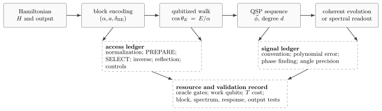
The Hamiltonian reaches QSP only through a normalized, executable block encoding. Qubitization maps $E/\alpha$ to a two-dimensional walk phase, and a degree-$d$ phase sequence implements the selected polynomial response. Normalization, oracle expansion, approximation, phase synthesis, and output costs remain attached to the result.

Convention warning

Some constructions use $U_HR$ instead of $RU_H$, choose $R=I-2\Pi$, or encode $x_E$ as $\sin\theta_E$ rather than $\cos\theta_E$. These conventions are equivalent after appropriate basis, sign, and phase changes, but their QSP phase lists are not interchangeable. A reproducible implementation must state the signal matrix, multiplication order, reflection sign, and phase-rotation convention.

Quantum Signal Processing

The invariant plane reduces the operator problem to controlled manipulation of one real signal $x\in[-1,1]$. A common abstract signal matrix is

$$S(x) = \begin{pmatrix} x & i\sqrt{1-x^2}\\ i\sqrt{1-x^2} & x \end{pmatrix}.$$

For a real phase list

$$\boldsymbol\phi = (\phi_0,\phi_1,\ldots,\phi_d),$$

define

$$V_{\boldsymbol\phi}(x) = e^{i\phi_0Z} \prod_{j=1}^{d} \left[ S(x)e^{i\phi_jZ} \right].$$

The order of the product is part of the convention. Each matrix element of $V_{\boldsymbol\phi}(x)$ is a polynomial in $x$ and $\sqrt{1-x^2}$ of degree at most $d$. In a standard form,

$$V_{\boldsymbol\phi}(x) = \begin{pmatrix} P(x) & iQ(x)\sqrt{1-x^2}\\ iQ^*(x)\sqrt{1-x^2} & P^*(x) \end{pmatrix}.$$

Unitarity imposes

$$|P(x)|^2 + (1-x^2)|Q(x)|^2 = 1$$

for real $x\in[-1,1]$. The degree and parity obey

$$\deg P\leq d, \qquad P(-x)=(-1)^dP(x),$$

with the complementary polynomial having the corresponding opposite parity. The exact reality and reciprocity conditions depend on the QSP convention.

Why arbitrary polynomial coefficients are not enough

A proposed polynomial is not implementable merely because its degree is small. It must satisfy:

1. the parity required by the sequence length;
2. boundedness or a unitary completion on $[-1,1]$;
3. the convention’s reality and endpoint conditions;
4. a numerically realizable phase factorization;
5. sufficient coefficient and angle precision.

If a target lacks definite parity, it can often be decomposed into even and odd parts and combined coherently, or implemented in an equivalent generalized QSP convention. Hamiltonian evolution is a canonical example:

$$e^{-i\tau x} = \cos(\tau x)-i\sin(\tau x),$$

where the real part is even and the imaginary part is odd.

Chebyshev interpretation

Write

$$x=\cos\theta.$$

Then

$$T_k(x)=\cos(k\theta),$$

so repeated signal rotations naturally generate Chebyshev modes. This is the link between single-qubit phase sequences and polynomial approximation on an entire Hamiltonian spectrum. QSP does not estimate $x$ and classically compute $f(x)$; it transforms all occupied spectral components coherently.

Hamiltonian Evolution as a Polynomial

The target normalized response is

$$f_\tau(x)=e^{-i\tau x}, \qquad \tau=\frac{\alpha t}{\hbar}.$$

Using $x=\cos\theta$, the Jacobi–Anger expansion gives

$$e^{-i\tau\cos\theta} = J_0(\tau) + 2\sum_{k=1}^{\infty} (-i)^kJ_k(\tau)\cos(k\theta),$$

or equivalently

$$e^{-i\tau x} = J_0(\tau) + 2\sum_{k=1}^{\infty} (-i)^kJ_k(\tau)T_k(x).$$

Here $J_k$ is a Bessel function of the first kind. Truncating at degree $d$ gives a uniform error bounded by the Bessel tail,

$$\epsilon_{\mathrm{poly}} \leq 2\sum_{k=d+1}^{\infty}|J_k(\tau)|.$$

The coefficients decay rapidly once $k$ exceeds the effective bandwidth set by $|\tau|$. This is why the degree grows approximately linearly with normalized time and only mildly with inverse precision.

Query-optimal degree

For $\tau>0$ and $0<\epsilon<1$, the optimal joint scaling can be written

$$d = O\!\left[ \tau + \frac{ \log(1/\epsilon) }{ \log\!\left( e+\log(1/\epsilon)/\tau \right) } \right].$$

A simpler but weaker summary is

$$d = O\!\left( \tau+\log(1/\epsilon) \right).$$

The first expression captures two limits:

• for long evolution at fixed precision, $d=O(\tau)$;
• for very high precision at modest $\tau$, the precision contribution is approximately $O(\log(1/\epsilon)/\log\log(1/\epsilon))$.

Under the standard block-encoding query model, matching lower bounds make the joint dependence query optimal up to constants and convention details. This does not contradict no-fast-forwarding: generic black-box Hamiltonians still require a number of queries linear in $\alpha|t|/\hbar$.

What one query means

A degree-$d$ QSP sequence uses $O(d)$ calls to its signal operation, with the exact count depending on parity, completion, and whether the sequence alternates $W$ and $W^\dagger$. It also uses $d+1$ phase rotations. Query optimality therefore says nothing yet about the elementary-gate cost of one walk call.

Worked Example: Two Pauli Terms

Consider

$$H=aX+bZ, \qquad a,b\in\mathbb R.$$

An LCU encoding has

$$\lambda=|a|+|b|,$$

coefficient state

$$\lvert G\rangle = \sqrt{\frac{|a|}{\lambda}}\lvert0\rangle + \sqrt{\frac{|b|}{\lambda}}\lvert1\rangle,$$

and

$$\operatorname{SELECT} = \lvert0\rangle\langle0\rvert \otimes\operatorname{sgn}(a)X + \lvert1\rangle\langle1\rvert \otimes\operatorname{sgn}(b)Z.$$

The compression is $H/\lambda$. The physical eigenvalues are

$$E_\pm=\pm\Omega, \qquad \Omega=\sqrt{a^2+b^2},$$

and the qubitized walk phases obey

$$\cos\theta_\pm = \frac{E_\pm}{\lambda} = \pm\frac{\Omega}{\lambda}.$$

QSP targets

$$e^{-i\tau(E_\pm/\lambda)} = e^{-iE_\pm t/\hbar}, \qquad \tau=\frac{\lambda t}{\hbar}.$$

If $a$ and $b$ are both nonzero, then

$$\lambda>\Omega=\|H\|.$$

For $a=b\ne0$,

$$\frac{\lambda}{\|H\|} = \sqrt2.$$

The walk therefore processes a normalized time $\sqrt2$ larger than the minimum spectral scale would suggest. If one coefficient vanishes, the ratio becomes one and a direct Pauli rotation is already exact. Qubitization remains valid in that limit, but it is not the sensible implementation.

Direct Spectral Readout from the Walk

QSP is not the only use of the qubitized walk. Controlled phase estimation on $W$ can estimate $\theta_E$ directly, then recover

$$E=\alpha\cos\theta_E.$$

The lifted state is

$$\lvert g_E\rangle = \frac{ \lvert w_{E,+}\rangle + \lvert w_{E,-}\rangle }{\sqrt2}.$$

Phase estimation can therefore return either branch $+\theta_E$ or $-\theta_E$. Both give the same energy after applying cosine. For a small phase error $\delta\theta$,

$$\delta E \approx -\alpha\sin\theta_E\,\delta\theta,$$

and hence

$$|\delta E| \leq \alpha|\delta\theta| +O(\delta\theta^2).$$

Direct walk-based phase estimation avoids first compiling a long-time exponential, but it still requires a trial-state overlap with the desired eigenstate, controlled walk powers, phase-unwrapping conventions, and enough coherent queries to resolve the energy. The block normalization again sets the natural energy scale.

Approximate Encodings and Robustness

Suppose the selected block corresponds to an effective Hamiltonian $\widetilde H$ with

$$\|H-\widetilde H\| \leq \delta_{\mathrm{BE}}.$$

Duhamel’s formula gives

$$\left\| e^{-iHt/\hbar} - e^{-i\widetilde Ht/\hbar} \right\| \leq \frac{|t|}{\hbar} \delta_{\mathrm{BE}}.$$

This contribution is separate from polynomial approximation. If the realized signal query $\widetilde W$ satisfies

$$\|W-\widetilde W\|\leq\eta_W,$$

then a degree-$d$ sequence has the coarse telescoping bound

$$\epsilon_W \leq d\eta_W.$$

Likewise, if the $j$th phase rotation has operator error $\eta_{\phi,j}$,

$$\epsilon_\phi \leq \sum_{j=0}^{d}\eta_{\phi,j}.$$

A conservative ideal-to-real ledger is therefore

$$\begin{aligned} \epsilon_{\mathrm{coh}} \leq{}& \frac{|t|}{\hbar}\delta_{\mathrm{BE}} +\epsilon_{\mathrm{poly}} +d\eta_W \\ &+ \sum_{j=0}^{d}\eta_{\phi,j} +\epsilon_{\mathrm{ctrl}} +\epsilon_{\mathrm{compile}}. \end{aligned}$$

This is a worst-case budget, not a prediction that coherent errors add incoherently or with the same sign. Model reduction, state preparation, fault-tolerant logical failure, and measurement statistics must be added at their own interfaces.

Allocating precision

For a target coherent error $\epsilon$, one possible allocation is

$$\frac{|t|}{\hbar}\delta_{\mathrm{BE}} \leq \frac{\epsilon}{4}, \qquad \epsilon_{\mathrm{poly}} \leq \frac{\epsilon}{4},$$

and

$$d\eta_W \leq \frac{\epsilon}{4}, \qquad \sum_{j=0}^{d}\eta_{\phi,j} \leq \frac{\epsilon}{4}.$$

Equal allocation is not generally cost optimal. If PREPARE precision is expensive while axial rotations are cheap, the best budget can be highly uneven. Resource optimization should minimize physical cost subject to the total error constraint.

Phase Finding Is Part of the Algorithm

Polynomial design and phase finding are distinct classical tasks:

1. choose or compute an admissible polynomial approximating the target;
2. complete it to a unitary QSP response;
3. factor that response into phases $\boldsymbol\phi$;
4. verify the phases in the exact circuit convention to be used;
5. round or synthesize them to the allocated precision.

High-degree phase recovery can be numerically delicate. Root-based methods may require extended precision; optimization, Prony-like, fixed-point, and structured-factorization methods have improved the stable range. A claimed degree is not yet an executable circuit if no phase list has been generated and checked.

For a computed list, reconstruct the realized response on a dense spectral grid and, when a rigorous guarantee is required, supplement sampling with an interval or coefficient-based error certificate. Grid agreement alone can miss a narrow excursion between points.

Phase precision and non-Clifford cost

If $d+1$ arbitrary axial rotations each receive tolerance of order $\epsilon_\phi/(d+1)$, a representative fault-tolerant synthesis cost is

$$N_T^{(\phi)} = O\!\left[ d\log\!\left( \frac{d}{\epsilon_\phi} \right) \right],$$

up to synthesis method and gate-set constants. This can be smaller than the oracle cost, but it is not zero. Phase-gradient states, repeat-until-success methods, catalysis, or native logical rotations change the ledger and must be named.

Expanding Queries into Fault-Tolerant Resources

For the LCU construction,

$$C_{U_H} = C_{\mathrm{PREPARE}} +C_{\mathrm{SELECT}} +C_{\mathrm{PREPARE}^\dagger}.$$

One walk call also requires the reflection $R$. A degree-$d$ implementation therefore has a schematic logical cost

$$C_{\mathrm{QSP}} \approx d\left( C_{U_H}+C_R \right) +C_{\mathrm{phase}} +C_{\mathrm{control}} +C_{\mathrm{boundary}}.$$

The exact constants depend on whether the sequence uses $W$, $W^\dagger$, alternating phase conventions, parity completion, and postselection or oblivious amplification.

PREPARE

PREPARE may require:

• QROM or arithmetic for coefficient data;
• alias sampling or inequality tests;
• reversible normalization and square-root approximations;
• work registers that must be uncomputed;
• precision sufficient to meet $\delta_{\mathrm{BE}}$.

Its qubit and Toffoli costs can dominate. Treating an arbitrary coefficient state as one elementary gate is an oracle-model statement, not a physical resource estimate.

SELECT

SELECT may require:

• multiplexed Pauli strings or fermionic operations;
• address decoding and swaps;
• basis rotations and parity networks;
• reversible evaluation of sparse indices;
• additional controls for phase estimation.

Symmetry, low-rank factorization, unary iteration, and data layout can change both normalization and gate cost. The best encoding is therefore application and architecture dependent.

Reflection and controls

The reflection

$$R=2\Pi-I$$

is a multi-register phase conditioned on all block ancillas being zero. Its cost depends on available clean or dirty ancillas and the fault-tolerant gate set. If the QSP simulator will be controlled, the global phase convention and every oracle control must be implemented consistently; a phase that is global for the uncontrolled unitary becomes relative between control branches.

Ancilla accounting

QSP and qubitization need only a small number of signal-processing ancillas beyond the block encoding. This does not mean the complete algorithm uses a constant number of ancillas. PREPARE, SELECT, QROM, arithmetic, phase estimation, error correction, and magic-state factories can require many more.

Energy Shifts and Rescaling

For a known scalar $c$,

$$H=\left(H-cI\right)+cI$$

and

$$e^{-iHt/\hbar} = e^{-ict/\hbar} e^{-i(H-cI)t/\hbar}.$$

If shifting the identity reduces the available block normalization from $\alpha$ to $\alpha(c)$, it can reduce QSP degree. The scalar phase can be discarded for an uncontrolled channel, but must be restored for controlled evolution, interferometry, and absolute phase estimation.

The optimization should minimize the implemented cost

$$d\!\left( \frac{\alpha(c)|t|}{\hbar}, \epsilon \right) C_{\mathrm{query}}(c),$$

not merely the spectral radius of $H-cI$. An LCU decomposition may respond to the identity shift differently from an abstract optimal block encoding.

Comparison with Product Formulas

Product formulas and qubitization consume different access primitives.

Feature	Trotter–Suzuki	Qubitization and QSP
required access	exponentials of Hamiltonian terms	coherent block encoding, inverse, reflection, and controls
main structural parameter	nested commutators, locality, ordering	normalization $\alpha$ and query implementation cost
precision dependence	polynomial for fixed order	near-logarithmic query contribution
ancillas	often few	few signal ancillas, potentially many oracle work qubits
natural setting	local/native terms, moderate precision	fault-tolerant coherent access, high precision
chief practical risk	many term rotations and routed depth	expensive PREPARE/SELECT and controlled oracle expansion

Qubitization is compelling when a favorable block encoding is already known, its queries compile efficiently, and high coherent accuracy is valuable. Product formulas can win when local exponentials are native, commutators are sparse, precision is moderate, or coherent data access is expensive. The comparison must use the same Hamiltonian truncation, output, tolerance, architecture, and failure probability.

Trotter–Suzuki Methods develops the product-formula side of this comparison.

Validation Workflow

Qubitization has several independently testable interfaces.

Validate the block

On small instances or structured test vectors, check

$$\alpha \left( \langle0^a\rvert\otimes I \right) U_H \left( \lvert0^a\rangle\otimes I \right) \approx H.$$

Also verify:

• normalization of PREPARE and its inverse;
• unitarity and, when assumed, Hermiticity of SELECT;
• coefficient signs and fixed-point precision;
• garbage-register cleanup;
• controlled and uncontrolled versions in the same convention.

Validate the walk spectrum

For exact diagonalizable examples, compare each eigenvalue pair of $W$ with

$$e^{\pm i\arccos(E/\alpha)}.$$

Test interior eigenvalues and endpoints near $E=\pm\alpha$. Check that the encoded eigenstate lies in the predicted invariant subspace and that leakage arises only from the declared approximate encoding or implementation error.

Validate the QSP response

For the generated phase list:

1. reconstruct $V_{\boldsymbol\phi}(x)$ numerically;
2. compare the selected response with $e^{-i\tau x}$ over $[-1,1]$;
3. verify parity, unitarity, and complementary-polynomial identities;
4. repeat after rounding phases to their compiled precision;
5. compare the complete circuit against exact evolution on small systems.

Validate the output

A small full-unitary error is useful but not a complete scientific validation. Check the requested state, observable, correlation function, or energy against an exact solver, tensor network, perturbative limit, conserved quantity, or other trusted baseline. State preparation and readout uncertainty belong in the same final claim.

Reporting Checklist

Item	Required information
target	Hamiltonian, units, time, input state, and requested output
encoding	$\alpha$, ancilla count, block error, PREPARE, SELECT, data layout, and coefficient precision
convention	projector, reflection sign, walk order, signal matrix, phase-rotation definition, and global phase
polynomial	target function, interval, degree, parity construction, approximation method, and certified error
phases	phase-finding method, arithmetic precision, angle list or reproducible artifact, and post-rounding error
queries	counts of $U_H$, $U_H^\dagger$, reflections, controls, PREPARE, SELECT, and any amplification
logical resources	Clifford, non-Clifford, depth, work qubits, QROM, and controlled-query costs
physical resources	code distance, logical failure budget, factories, physical qubits, runtime, and architecture
validation	block tests, walk spectrum, QSP response, exact small instances, and output-level baseline

Common Mistakes

• Quoting $O(\alpha t+\log(1/\epsilon))$ without defining $\alpha$ or the block-encoding query.
• Treating PREPARE or QRAM access as free because it appears once in an oracle diagram.
• Assuming every block encoding is already a Hermitian involution.
• Mixing $RU_H$ with $U_HR$, or sine and cosine signal conventions, while reusing the same phase list.
• Calling any polynomial approximation a valid QSP response without checking parity, boundedness, and unitary completion.
• Reporting the polynomial degree before generating and validating phases.
• Ignoring phase-rounding and signal-query errors that accumulate with degree.
• Counting only the constant number of signal ancillas while omitting oracle, arithmetic, phase-estimation, and error-correction work qubits.
• Dropping an energy-shift phase in a controlled simulation.
• Treating walk phase estimation as deterministic on $\lvert0^a\rangle\lvert E\rangle$; both $\pm\theta_E$ branches are present.
• Comparing abstract block-encoding queries with routed product-formula gates.
• Inferring an application advantage before including state preparation, measurement, retries, and a matched classical baseline.

Knowledge Status

The invariant-subspace construction, QSP polynomial characterization, Hamiltonian-simulation algorithms, and query lower bounds are established results under their stated oracle models. The distinction between query and gate complexity is not a caveat to those theorems; it is part of applying them to a physical architecture.

Encoding design, phase-factor generation at extreme degree, compiler-aware oracle optimization, low-rank chemistry constructions, rotation synthesis, and end-to-end fault-tolerant comparison remain active engineering and research areas. Resource improvements for one basis, data structure, or logical architecture should not be transferred to another without rebuilding the ledger.

References

1. G. H. Low, T. J. Yoder, and I. L. Chuang, “Methodology of Resonant Equiangular Composite Quantum Gates,” Physical Review X 6, 041067 (2016), doi:10.1103/PhysRevX.6.041067.
2. G. H. Low and I. L. Chuang, “Optimal Hamiltonian Simulation by Quantum Signal Processing,” Physical Review Letters 118, 010501 (2017), doi:10.1103/PhysRevLett.118.010501.
3. G. H. Low and I. L. Chuang, “Hamiltonian Simulation by Qubitization,” Quantum 3, 163 (2019), doi:10.22331/q-2019-07-12-163.
4. A. Gilyén, Y. Su, G. H. Low, and N. Wiebe, “Quantum Singular Value Transformation and Beyond: Exponential Improvements for Quantum Matrix Arithmetics,” in Proceedings of the 51st Annual ACM SIGACT Symposium on Theory of Computing, 193–204 (2019), doi:10.1145/3313276.3316366.
5. J. Haah, “Product Decomposition of Periodic Functions in Quantum Signal Processing,” Quantum 3, 190 (2019), doi:10.22331/q-2019-10-07-190.
6. Y. Dong, X. Meng, K. B. Whaley, and L. Lin, “Efficient Phase-Factor Evaluation in Quantum Signal Processing,” Physical Review A 103, 042419 (2021), doi:10.1103/PhysRevA.103.042419.
7. L. Ying, “Stable Factorization for Phase Factors of Quantum Signal Processing,” Quantum 6, 842 (2022), doi:10.22331/q-2022-10-20-842.
8. J. M. Martyn, Z. M. Rossi, A. K. Tan, and I. L. Chuang, “Grand Unification of Quantum Algorithms,” PRX Quantum 2, 040203 (2021), doi:10.1103/PRXQuantum.2.040203.
9. D. W. Berry, A. M. Childs, R. Cleve, R. Kothari, and R. D. Somma, “Simulating Hamiltonian Dynamics with a Truncated Taylor Series,” Physical Review Letters 114, 090502 (2015), doi:10.1103/PhysRevLett.114.090502.
10. D. W. Berry, A. M. Childs, and R. Kothari, “Hamiltonian Simulation with Nearly Optimal Dependence on All Parameters,” in 2015 IEEE 56th Annual Symposium on Foundations of Computer Science, 792–809 (2015), doi:10.1109/FOCS.2015.54.
11. D. W. Berry, C. Gidney, M. Motta, J. R. McClean, and R. Babbush, “Qubitization of Arbitrary Basis Quantum Chemistry Leveraging Sparsity and Low Rank Factorization,” Quantum 3, 208 (2019), doi:10.22331/q-2019-12-02-208.
12. R. Babbush et al., “Encoding Electronic Spectra in Quantum Circuits with Linear $T$ Complexity,” Physical Review X 8, 041015 (2018), doi:10.1103/PhysRevX.8.041015.
13. D. Camps, L. Lin, R. Van Beeumen, and C. Yang, “Explicit Quantum Circuits for Block Encodings of Certain Sparse Matrices,” SIAM Journal on Matrix Analysis and Applications 45, 801–827 (2024), doi:10.1137/22M1484298.
14. L. Lin, “Lecture Notes on Quantum Algorithms for Scientific Computation,” arXiv:2201.08309 (2022), doi:10.48550/arXiv.2201.08309.
15. A. M. Childs, “On the Relationship Between Continuous- and Discrete-Time Quantum Walk,” Communications in Mathematical Physics 294, 581–603 (2010), doi:10.1007/s00220-009-0930-1.

Further Connections

• Hamiltonian Simulation defines block-encoding access, normalized time, generic error propagation, and comparisons with other simulation families.
• Algorithmic Primitives gives the compact reusable language for block encoding, QSP, QSVT, phase estimation, amplification, and postselection.
• Digital Quantum Simulation places the signal-processing primitive inside representation, state preparation, compilation, execution, and readout.
• Quantum Phase Estimation owns finite-resolution phase statistics, controlled powers, overlap, aliasing, and total interrogation time.
• Universal Gate Sets explains why arbitrary QSP phase rotations require approximation in a fault-tolerant gate alphabet.
• Resource Estimation Tools expands logical circuits into architecture-dependent physical resources.
• Quantum Error-Correction Resource Estimation owns code distance, logical failure, magic-state factories, physical qubits, and runtime assumptions.
• Simulation of Quantum Chemistry explains how orbital representations and integral factorizations determine chemistry block encodings, normalizations, input states, and output claims.
• Simulation of Quantum Materials explains how periodic bases, downfolded interactions, translation structure, extensive precision, input states, and material observables determine block-encoding costs and claims.
• Quantum Chemistry Case Studies examines how Hamiltonian representation and oracle construction shape concrete chemistry estimates.

Exercises

1. Verify the LCU block

For

$$H=\sum_\ell h_\ell P_\ell,$$

use the PREPARE and SELECT definitions on this page to prove that the selected block is $H/\lambda$.

Solution

Insert the coefficient state on both sides of SELECT:

$$\begin{aligned} &\left( \langle G\rvert\otimes I \right) \operatorname{SELECT} \left( \lvert G\rangle\otimes I \right) \\ &= \sum_{j,k,\ell} \sqrt{\frac{|h_j|}{\lambda}} \sqrt{\frac{|h_k|}{\lambda}} \langle j\vert\ell\rangle \langle\ell\vert k\rangle \operatorname{sgn}(h_\ell)P_\ell \\ &= \sum_\ell \frac{|h_\ell|}{\lambda} \operatorname{sgn}(h_\ell)P_\ell = \frac{H}{\lambda}. \end{aligned}$$

Conjugating SELECT by PREPARE moves $\lvert G\rangle$ to the all-zero ancilla state without changing the compressed operator.

2. Derive the invariant-plane matrix

Starting from

$$U_H\lvert g\rangle=x\lvert g\rangle+s\lvert b\rangle, \qquad s=\sqrt{1-x^2},$$

and $U_H^2=I$, derive the action of $U_H$ on $\lvert b\rangle$ and the matrix of $W=RU_H$.

Solution

By definition,

$$s\lvert b\rangle = U_H\lvert g\rangle-x\lvert g\rangle.$$

Apply $U_H$ and use $U_H^2=I$:

$$\begin{aligned} sU_H\lvert b\rangle &= \lvert g\rangle-xU_H\lvert g\rangle \\ &= (1-x^2)\lvert g\rangle-xs\lvert b\rangle. \end{aligned}$$

Thus

$$U_H\lvert b\rangle = s\lvert g\rangle-x\lvert b\rangle.$$

Since $R\lvert g\rangle=\lvert g\rangle$ and $R\lvert b\rangle=-\lvert b\rangle$,

$$W = \begin{pmatrix} x&s\\ -s&x \end{pmatrix}$$

in the ordered basis $(\lvert g\rangle,\lvert b\rangle)$.

3. Recover energy from a walk phase

Suppose phase estimation returns $\widetilde\theta$ with $|\widetilde\theta-\theta_E|\leq\delta_\theta$. Bound the resulting energy error for $\widetilde E=\alpha\cos\widetilde\theta$.

Solution

The mean-value theorem gives

$$|\widetilde E-E| = \alpha |\cos\widetilde\theta-\cos\theta_E| \leq \alpha\delta_\theta,$$

because $|\sin\theta|\leq1$. Locally,

$$\widetilde E-E = -\alpha\sin\theta_E (\widetilde\theta-\theta_E) +O(\delta_\theta^2).$$

The local sensitivity is smaller near $E=\pm\alpha$, but phase-branch and finite-resolution issues must still be handled.

4. Propagate block-encoding error

An approximate block encoding represents $\widetilde H$ with $\|H-\widetilde H\|\leq\delta$. Show that choosing

$$\delta\leq\frac{\hbar\epsilon}{4|t|}$$

allocates at most $\epsilon/4$ to the induced evolution error.

Solution

Duhamel’s formula and unitary invariance give

$$\left\| e^{-iHt/\hbar} -e^{-i\widetilde Ht/\hbar} \right\| \leq \frac{|t|}{\hbar} \|H-\widetilde H\|.$$

Substituting the proposed bound on $\delta$ yields

$$\frac{|t|}{\hbar}\delta \leq \frac{\epsilon}{4}.$$

5. Account for phase-rotation precision

A degree-$d$ sequence has $d+1$ phase rotations. If each realized rotation is within operator norm $\eta$ of its ideal value, give a sufficient per-rotation tolerance for a total phase-synthesis budget $\epsilon_\phi$.

Solution

A telescoping product bound gives

$$\epsilon_\phi \leq (d+1)\eta.$$

It is therefore sufficient to choose

$$\eta \leq \frac{\epsilon_\phi}{d+1}.$$

This uniform allocation is convenient, not necessarily cost optimal. Some angles may synthesize exactly or more cheaply than others.

6. Optimize a scalar shift

Explain why minimizing $\|H-cI\|$ need not minimize the fault-tolerant cost of qubitization. What must be compared instead?

Solution

The available block normalization $\alpha(c)$ need not equal $\|H-cI\|$. It depends on the chosen decomposition and data structure. The identity shift can also change PREPARE, SELECT, arithmetic, and phase-correction costs. The relevant comparison is therefore something like

$$d\!\left( \frac{\alpha(c)|t|}{\hbar}, \epsilon \right) C_{\mathrm{query}}(c) +C_{\mathrm{phase\ correction}}(c),$$

with the scalar phase restored whenever the simulation is controlled or used interferometrically.

7. Audit an ancilla claim

A paper says that qubitization uses “only two ancilla qubits.” List the registers that must be checked before interpreting this as an end-to-end qubit count.

Solution

The quoted number may count only additional signal-processing ancillas. An end-to-end audit must also include:

1. the Hamiltonian block-encoding index register;
2. PREPARE and SELECT work registers;
3. QROM address, data, alias-sampling, and arithmetic registers;
4. phase-estimation controls, if used;
5. uncomputation and routing ancillas;
6. logical encoding overhead;
7. magic-state factories and routing space in the physical architecture.

The appropriate total depends on the specific oracle and fault-tolerance design.

8. Compare access models

A local Hamiltonian has cheap native term exponentials but an LCU block encoding with large $\lambda$ and expensive QROM. Explain why the asymptotic precision advantage of QSP does not by itself determine the best method.

Solution

QSP uses roughly

$$d=d(\lambda|t|/\hbar,\epsilon)$$

coherent signal queries, each of which expands into PREPARE, SELECT, reflection, uncomputation, controls, and phase rotations. A product formula uses term exponentials whose count depends on commutators, locality, order, and the target output. For moderate precision, small commutator coefficients and cheap native exponentials can outweigh QSP’s superior asymptotic dependence on $\epsilon$. A fair comparison compiles both methods to the same architecture and includes state preparation, output extraction, and the same error budget.