Open-System Simulation

Short Definition

Open-system quantum simulation is the controlled reproduction of a target nonunitary quantum process on a programmable or purpose-built quantum device. The target may be a quantum channel, a time-dependent Lindblad generator, a microscopic system–environment model, or a monitored stochastic process. A credible simulation specifies which degrees of freedom are retained, how the environment is represented, which observables are estimated, and how target dissipation is separated from uncontrolled simulator noise.

The word open does not by itself identify a mathematical model. Markovian dynamics, a finite memory kernel, a structured quantum bath, classical stochastic driving, and postselected non-Hermitian evolution are different targets. They need different implementations and support different claims.

Canonical Scope

This page is the canonical home for the simulation workflow:

• converting a specified open process into executable quantum operations;
• choosing among channel dilation, Liouvillian simulation, trajectories, collision models, and engineered reservoirs;
• accounting for ancillas, resets, bath modes, trajectories, and shots;
• validating physicality, dynamics, steady states, and observables; and
• bounding target-model, compilation, hardware, and statistical errors.

The underlying theory remains canonical elsewhere:

• Kraus representations and Stinespring representations explain quantum channels and their dilations;
• the Lindblad–GKSL equation develops Markovian generators;
• collision models develop repeated-interaction dynamics and memory mechanisms;
• unravelings and quantum-jump trajectories develop conditional stochastic descriptions; and
• reservoir engineering develops dissipation as a control resource.

Here those objects are treated as simulation specifications. The question is not merely whether a map is mathematically valid, but whether a device implements it with controlled cost and error over the claimed regime.

Why Open-System Simulation Is Distinct

A closed-system simulator approximates a unitary operator. An open-system simulator must reproduce a map on density operators,

$$\rho(0) \longmapsto \rho(t) = \Phi_{t:0}[\rho(0)],$$

usually while exposing or discarding additional degrees of freedom. This creates several obligations absent from ordinary Hamiltonian simulation.

Physicality is part of the target

For an initially uncorrelated system and environment, every finite-time reduced map must be completely positive and trace preserving (CPTP). A numerical approximation that preserves trace but produces a negative Choi eigenvalue is not simply imprecise; it may fail to describe a physical channel.

Irreversibility consumes resources

Unitary gates do not erase information. A digital implementation of damping therefore stores entropy in ancillas, measurements, resets, classical records, or uncontrolled environmental modes. The location of that information is a resource-accounting question.

The simulator is already open

Every laboratory device has its own relaxation, dephasing, leakage, drift, and measurement errors. Those processes do not automatically implement the target environment. Useful target loss and parasitic hardware loss may have the same qualitative signature while differing in rate, locality, temperature, correlations, and dependence on control settings.

Output remains an observable, not a density matrix

An $n$-qubit density matrix contains $4^n-1$ real parameters. Efficient state evolution does not imply efficient full-state readout. A simulation claim must therefore name an observable family or operational task whose measurement cost is included.

Specify the Simulation Contract

Before choosing an algorithm or platform, record the following objects.

Retained system

Specify the Hilbert space $\mathcal H_S$, any truncations, and the subsystem called the environment. A bosonic mode treated explicitly in one calculation may be part of an effective bath in another. This partition changes both the state and the meaning of memory.

Initial condition

The usual reduced-map statement assumes

$$\rho_{SE}(0) = \rho_S(0)\otimes\tau_E.$$

If the system and environment are initially correlated, a single CPTP map on all possible system inputs need not exist. The preparation procedure or assignment map must then be part of the specification; see initial correlations.

Dynamical representation

State exactly one primary target:

1. a channel $\Phi_{t:0}$ at one or more times;
2. a time-local generator $\mathcal L_t$;
3. a system–environment Hamiltonian $H_{SE}(t)$ and bath state;
4. a process with memory across interventions; or
5. a monitored instrument with classical outcome records.

These descriptions can be related under assumptions, but they are not interchangeable data structures. Matching $\Phi_{t:0}$ at a few times does not prove that the implemented process has the intended multitime correlations.

Controls and interventions

Declare Hamiltonian drives, measurements, feedback, resets, and the times at which an experimenter may intervene. For a driven Markovian model,

$$\frac{d\rho}{dt} = \mathcal L_t(\rho) = -\frac{i}{\hbar}[H(t),\rho] + \sum_\mu \mathcal D[L_\mu(t)]\rho,$$

with

$$\mathcal D[L]\rho = L\rho L^\dagger - \frac12\{L^\dagger L,\rho\}.$$

The assumptions behind a driven master equation are discussed in Driven Open Systems.

Observables and time window

Name the requested quantities,

$$f_j(t) = \operatorname{Tr}[O_j\rho(t)], \qquad 0\le t\le T,$$

or a steady-state, first-passage, correlation, or response quantity. The norm, resolution, and desired confidence interval belong in the contract.

Error metric

For a state-specific claim, trace distance may be enough. For a uniform channel claim, use a stabilized norm such as

$$\epsilon_\diamond(t) = \left\| \widetilde\Phi_{t:0}-\Phi_{t:0} \right\|_\diamond.$$

The diamond norm includes an arbitrary reference system and therefore controls the channel on entangled inputs. Report the convention explicitly: some authors place a factor of $1/2$ in the operational channel distance.

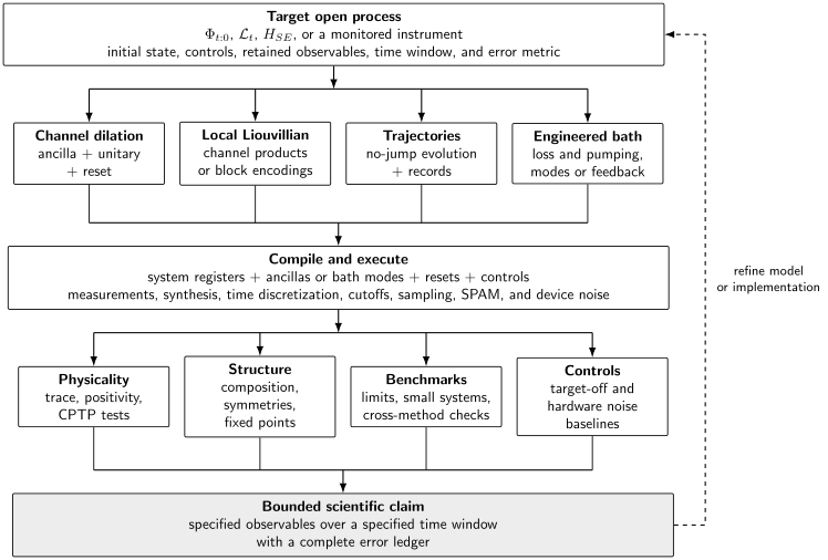
An open-system simulator is an evidence pipeline. The representation controls which resources carry entropy and memory; validation must test both the target process and the distinction between engineered and parasitic noise.

Choose an Implementation Route

No route dominates for every target. The correct choice depends on whether the goal is finite-time channel action, long-time steady behavior, monitored records, or microscopic bath physics.

Route	Natural target	Main resources	Characteristic limitation
Channel dilation	A known CPTP map or short-time channel	Ancillas, controlled unitaries, discard or reset	Dilation synthesis and repeated reset cost
Local Liouvillian composition	Local Markovian dynamics	Channel primitives, time steps, gates	Product and synthesis error
Quantum trajectories	Sparse jumps and conditional records	Repetitions, mid-circuit measurements or classical sampling	Trajectory variance and rare events
Collision model	Repeated interactions and designed memory	Fresh, correlated, or recycled ancillas	Ancilla supply and memory architecture
Engineered reservoir	Native dissipation or steady-state preparation	Lossy modes, pumping, feedback, calibration	Model inflexibility and parasitic processes
Explicit bath	Structured or non-Markovian environment	Bath modes, bosonic cutoffs, longer coherence	Bath discretization and finite recurrence

Hybrid schemes are common. A processor may digitally compile coherent terms, use native reset for jumps, and retain a small quantum memory representing the most important bath modes.

Channel Dilation

Let one simulation step be the channel

$$\mathcal E(\rho) = \sum_{a=0}^{r-1} K_a\rho K_a^\dagger, \qquad \sum_aK_a^\dagger K_a=I.$$

The Kraus rank $r$ is the rank of the channel’s Choi matrix. An isometric dilation acts as

$$V\lvert\psi\rangle_S\lvert0\rangle_E = \sum_{a=0}^{r-1} K_a\lvert\psi\rangle_S\lvert a\rangle_E.$$

Extending $V$ to a unitary $U$ on system plus environment gives

$$\mathcal E(\rho) = \operatorname{Tr}_E \left[ U(\rho\otimes\lvert0\rangle\langle0\rvert)U^\dagger \right].$$

At least $\lceil\log_2 r\rceil$ environment qubits are needed for a minimal pure-state dilation of a rank-$r$ finite-dimensional channel. A circuit may use more ancillas to reduce gate depth or simplify control.

Reset determines memory

To apply a memoryless channel repeatedly, the environment register must be discarded and replaced by the declared state after every step:

$$\rho_{j+1} = \mathcal E_j(\rho_j).$$

Reusing an entangled ancilla without reset generally changes later steps. The result is a correlated process, not another implementation of the original Markovian channel. Reuse can be valuable, but then the retained ancilla is a memory register and belongs in the model.

Dilation is not automatically efficient

Stinespring’s theorem proves existence, not a favorable circuit size. A dense channel on $n$ qubits can have Kraus rank as large as $4^n$, and a generic dilation unitary has exponential description complexity. Efficient simulation requires additional structure such as locality, sparsity, compact Kraus operators, a useful oracle, or native physical interactions.

Infinitesimal Channels from a Lindblad Generator

For a time-independent Lindblad generator with Hamiltonian $H$ and jump operators $L_\mu$, a short step $\delta t$ has the formal Kraus expansion

$$K_0 = I - \left( \frac{i}{\hbar}H + \frac12\sum_\mu L_\mu^\dagger L_\mu \right)\delta t +O(\delta t^2),$$

and

$$K_\mu = \sqrt{\delta t}\,L_\mu +O(\delta t^{3/2}).$$

Then

$$\sum_aK_a\rho K_a^\dagger = \rho+\delta t\,\mathcal L(\rho) +O(\delta t^2).$$

These truncated expressions are an asymptotic derivation, not an exact channel specification. At finite $\delta t$, simply dropping the remainder can violate trace preservation or positivity. A circuit needs an exactly CPTP completion, an exact primitive channel, or a quantitative bound on the implemented map.

One jump primitive

Suppose a jump operator has the form

$$L=\sqrt\gamma\,A, \qquad A^\dagger A\le I.$$

For small $p=\gamma\delta t$, one can seek a dilation whose ancilla-$1$ amplitude is $\sqrt p\,A\lvert\psi\rangle$. The complementary branch must be constructed so that

$$K_0^\dagger K_0+K_1^\dagger K_1=I$$

exactly. The Hamiltonian part and different dissipators can then be composed, provided the product error is included.

Compose Local Liouvillians

For a $k$-local Markovian model,

$$\mathcal L(t) = \sum_{\alpha=1}^{M}\mathcal L_\alpha(t),$$

each term acts on only a bounded number of neighboring subsystems. A first order channel product for a time-independent generator is

$$e^{t\mathcal L} \approx \left( e^{\delta t\mathcal L_M} \cdots e^{\delta t\mathcal L_1} \right)^m, \qquad \delta t=\frac tm.$$

Every exponential $e^{\delta t\mathcal L_\alpha}$ is CPTP when $\mathcal L_\alpha$ is itself a valid Lindblad generator. Thus the product is CPTP even before the time-step limit, although it approximates the target generator only up to noncommutativity errors.

Formally, the leading local error contains Liouvillian commutators,

$$e^{\delta t(\mathcal A+\mathcal B)} - e^{\delta t\mathcal B}e^{\delta t\mathcal A} = \frac{\delta t^2}{2}[\mathcal A,\mathcal B] +O(\delta t^3).$$

Norm bounds require care because superoperators need not be normal and their norms can scale with system size. Locality-sensitive estimates can be much tighter than a bound obtained by summing all global commutators.

The coherent analogue is developed in Trotter–Suzuki Methods. For open dynamics, the primitive factors must also remain physical channels.

What efficient-simulation theorems say

Under locality and boundedness assumptions, time-dependent local Liouvillian dynamics can be approximated by polynomial-size quantum circuits. More specialized algorithms achieve favorable precision dependence when the Hamiltonian and jump operators are supplied through sparse or linear-combination access models.

These are conditional complexity results. They do not imply that an arbitrary dense Lindblad matrix, supplied entry by entry, is efficiently simulable. State preparation, oracle construction, observable measurement, and fault-tolerant synthesis can dominate an application-level resource estimate.

Quantum-Trajectory Simulation

A Lindblad equation can be unraveled into stochastic pure-state trajectories. For quantum jumps, define the non-Hermitian effective Hamiltonian

$$H_{\mathrm{eff}} = H - \frac{i\hbar}{2} \sum_\mu L_\mu^\dagger L_\mu.$$

Between jumps, an unnormalized state evolves under $H_{\mathrm{eff}}$. During a short interval, jump $\mu$ occurs with probability

$$p_\mu = \delta t\, \langle\psi\rvert L_\mu^\dagger L_\mu\lvert\psi\rangle +O(\delta t^2),$$

after which

$$\lvert\psi\rangle \longmapsto \frac{L_\mu\lvert\psi\rangle} {\sqrt{\langle L_\mu^\dagger L_\mu\rangle}}.$$

The density operator is recovered as an ensemble average,

$$\rho(t) = \mathbb E \left[ \lvert\psi_\xi(t)\rangle \langle\psi_\xi(t)\rvert \right].$$

Two meanings of a trajectory experiment

1. A quantum device can implement a monitored dilation, measure the ancilla, and retain the outcome record. Each run is then a physical conditional trajectory.
2. A hybrid algorithm can sample jump times classically while a quantum processor implements conditional state evolution.

Both reproduce ensemble observables when their sampling law is correct. Only the first automatically claims the monitored record of a specified physical unraveling. Different measurements of the same environment produce different trajectory ensembles while leaving the unconditional master equation unchanged.

Sampling cost

For a trajectory estimator $X_\xi$ of an observable, the sample mean over $N_{\mathrm{traj}}$ independent runs has standard error

$$\operatorname{SE}(\overline X) = \sqrt{ \frac{\operatorname{Var}(X_\xi)} {N_{\mathrm{traj}}} }.$$

Rare jumps, first-passage events, and dynamical large deviations can require far more trajectories than ordinary local expectation values. Report both the number of trajectories and the measurement shots used within each trajectory.

Collision Models and Memory Registers

A collision model represents the environment by ancillas $E_1,E_2,\ldots$. For fresh independent ancillas in state $\tau_E$,

$$\rho_{j+1} = \operatorname{Tr}_{E_j} \left[ U_j(\rho_j\otimes\tau_E)U_j^\dagger \right].$$

This is a discrete Markovian process when each incoming ancilla is independent of the system and previous carriers. Memory can be introduced deliberately by:

• correlating the incoming ancillas;
• allowing ancilla–ancilla interactions;
• recycling a finite memory register;
• delaying measurements and feedforward; or
• retaining explicit bosonic or pseudomode degrees of freedom.

The memory depth is then a physical and computational parameter. A small memory register can compactly represent some structured environments, but no fixed register reproduces every long-memory bath over arbitrary times.

Multitime validation

Two implementations may agree on every one-time state $\rho(t_j)$ for one preparation and still respond differently to an intervention at an intermediate time. A non-Markovian simulation should therefore validate multitime statistics or intervention responses whenever those are part of the scientific claim. One-time state agreement alone does not identify a process with memory.

See What Non-Markovian Means for distinctions among memory, information backflow, and CP divisibility.

Explicit and Engineered Environments

Instead of compiling reduced channels, one may simulate a larger closed or weakly open model,

$$H_{SE} = H_S+H_E+H_{SE}^{\mathrm{int}},$$

and trace or ignore the explicit environment at readout.

Structured bosonic baths

A common target is

$$H_E = \sum_k\hbar\omega_k b_k^\dagger b_k, \qquad H_{SE}^{\mathrm{int}} = S\otimes \sum_k g_k(b_k+b_k^\dagger).$$

The continuum environment is characterized by a spectral density such as

$$J(\omega) = \pi\sum_k|g_k|^2\delta(\omega-\omega_k).$$

A finite simulator replaces that continuum by a finite set of modes or a mapped chain. It must control:

• frequency discretization and bandwidth;
• bosonic occupation cutoffs;
• preparation of thermal or squeezed bath states;
• finite-size recurrences;
• residual damping of the simulator modes; and
• the time interval before discretization artifacts return.

The spin–boson model, spectral densities, reaction-coordinate mappings, and pseudomode methods provide the theory behind these choices.

Reservoir engineering

An analog simulator may realize selected jump operators through optical pumping, lossy auxiliary modes, sympathetic cooling, controlled particle loss, or measurement and feedback. The target can be transient dynamics or an attractive steady state.

Native dissipation can greatly reduce circuit depth, but it shifts effort into calibration. One must show that the effective jump operators, rates, and bath state match the reduced model over the working range. Adiabatic elimination, rotating-wave, weak-coupling, and Markov approximations are part of the error ledger, not invisible hardware details.

Driven and Periodic Open Systems

For a time-dependent generator, the propagator is time ordered:

$$\Phi_{t:0} = \mathcal T \exp\left( \int_0^t\mathcal L_s\,ds \right).$$

Sampling $\mathcal L_t$ only at step boundaries introduces a control discretization error in addition to ordinary channel synthesis error. A midpoint or higher-order rule can improve time dependence without changing the spatial decomposition.

For a periodic generator $\mathcal L_{t+T}=\mathcal L_t$, the one-period map is

$$\mathcal F = \Phi_{T:0}.$$

A periodic steady regime satisfies

$$\mathcal F(\rho_F)=\rho_F, \qquad \rho_F(t+T)=\rho_F(t).$$

Validating only stroboscopic states can miss micromotion within each period. If intraperiod observables matter, they must be sampled and compared as part of the contract.

Worked Benchmark: Amplitude Damping

Amplitude damping is a useful exact benchmark because its finite-time channel, dilation, semigroup law, observables, and steady state are all known.

Target generator

Let $\lvert e\rangle$ decay to $\lvert g\rangle$ at rate $\gamma$,

$$\frac{d\rho}{dt} = \gamma \left( \sigma_-\rho\sigma_+ - \frac12\{\sigma_+\sigma_-,\rho\} \right),$$

where

$$\sigma_- = \lvert g\rangle\langle e\rvert.$$

Define

$$\eta(t)=e^{-\gamma t}.$$

The exact solution obeys

$$\rho_{ee}(t) = \eta(t)\rho_{ee}(0), \qquad \rho_{eg}(t) = \sqrt{\eta(t)}\rho_{eg}(0).$$

Exact finite-time channel

The Kraus operators are

$$K_0(t) = \lvert g\rangle\langle g\rvert + \sqrt{\eta(t)} \lvert e\rangle\langle e\rvert,$$ $$K_1(t) = \sqrt{1-\eta(t)} \lvert g\rangle\langle e\rvert.$$

They satisfy

$$K_0^\dagger K_0+K_1^\dagger K_1=I.$$

Thus the channel is CPTP for $0\le\eta\le1$. It also has the semigroup composition law

$$\mathcal E_{\eta_2} \circ \mathcal E_{\eta_1} = \mathcal E_{\eta_1\eta_2}.$$

One-ancilla dilation

Prepare an environment qubit in $\lvert0\rangle_E$ and implement a unitary whose relevant action is

$$\lvert g\rangle_S\lvert0\rangle_E \longmapsto \lvert g\rangle_S\lvert0\rangle_E,$$ $$\lvert e\rangle_S\lvert0\rangle_E \longmapsto \sqrt\eta\, \lvert e\rangle_S\lvert0\rangle_E + \sqrt{1-\eta}\, \lvert g\rangle_S\lvert1\rangle_E.$$

Tracing out the ancilla gives the target channel. Measuring the ancilla instead produces a jump record: outcome $1$ identifies a decay in the ideal dilation.

For a step $\delta t$, choose

$$\eta_\delta=e^{-\gamma\delta t}.$$

Resetting the ancilla after every step and applying the exact channel $m$ times gives

$$\eta_\delta^m = e^{-\gamma m\delta t} = e^{-\gamma t}.$$

For this isolated dissipator there is no time-discretization error at the channel level. Errors arise from dilation synthesis, ancilla preparation and reset, gates, measurements, and any additional Hamiltonian term that must be composed.

Observable checks

Using

$$Z = \lvert g\rangle\langle g\rvert - \lvert e\rangle\langle e\rvert,$$

the Bloch coordinates satisfy

$$x(t)=\sqrt\eta\,x(0), \qquad y(t)=\sqrt\eta\,y(0),$$ $$z(t) = 1-\eta+\eta z(0).$$

An implementation should recover:

• the identity map at $\gamma t=0$;
• the fixed point $\lvert g\rangle\langle g\rvert$;
• exponential excited-state decay;
• half-rate decay of coherence in the exponent;
• the semigroup composition law; and
• equality between the ancilla jump frequency and lost excited population.

Separate target decay from device decay

Suppose the hardware itself has amplitude-damping rate $\gamma_{\mathrm{hw}}$. In the simplest commuting approximation, an intended rate $\gamma_{\mathrm{tar}}$ may appear as

$$\gamma_{\mathrm{obs}} \approx \gamma_{\mathrm{tar}} + \gamma_{\mathrm{hw}}.$$

Agreement with a decaying exponential is therefore insufficient. Run a target-off control, vary the programmed rate, test input-state dependence, and propagate calibration uncertainty. For noncommuting noise or driven systems, rates need not add, so a composed channel model is required.

Steady States and Dissipative Preparation

A stationary state satisfies

$$\mathcal L(\rho_{\mathrm{ss}})=0.$$

If the stationary state is unique and attractive, dissipative evolution can prepare it without resolving an energy-minimization problem. For a target pure state $\lvert\psi_*\rangle$, a common design principle is

$$L_\mu\lvert\psi_*\rangle=0$$

for every jump operator, together with conditions excluding unwanted dark states.

Liouvillian gap

Let the Liouvillian eigenvalues satisfy $\lambda_0=0$ and $\operatorname{Re}\lambda_j\le0$. A commonly quoted asymptotic rate is

$$\Delta_{\mathcal L} = -\max_{j\ne0}\operatorname{Re}\lambda_j.$$

A small gap signals slow asymptotic relaxation. The gap alone need not bound all finite-time behavior tightly: non-normal generators, Jordan blocks, metastable manifolds, small stationary weights, and observable-dependent overlaps can create long transients. State-preparation costs should therefore be supported by measured or bounded mixing behavior, not only by one spectral number.

Residual test

For a reconstructed or classically represented candidate state, compute

$$r_{\mathrm{ss}} = \left\| \mathcal L(\widetilde\rho_{\mathrm{ss}}) \right\|_1.$$

A small residual is necessary but may not imply closeness when the generator is ill-conditioned or has nearly stationary modes. Combine it with uniqueness, gap or mixing information, direct observables, and initialization dependence.

Error Ledger

A useful decomposition is

$$\epsilon_{\mathrm{tot}} \lesssim \epsilon_{\mathrm{model}} + \epsilon_{\mathrm{bath}} + \epsilon_{\mathrm{time}} + \epsilon_{\mathrm{synth}} + \epsilon_{\mathrm{device}} + \epsilon_{\mathrm{SPAM}} + \epsilon_{\mathrm{stat}}.$$

This is an accounting scaffold, not an automatic theorem. Correlated errors may require a composed bound rather than a simple sum.

Model-reduction error

This includes Born, Markov, secular, rotating-wave, adiabatic-elimination, and weak-coupling approximations. A perfect simulation of an invalid reduced model does not validate the intended physical system.

Bath representation error

Explicit environments introduce mode discretization, bandwidth, occupation cutoffs, finite memory, and recurrence errors. Collision models introduce finite step size and finite memory depth.

Temporal decomposition error

Product formulas, sampled controls, and truncated short-time channels differ from the target propagator. Check convergence by decreasing $\delta t$ while holding other resources fixed as far as possible.

Channel-synthesis error

The compiled unitary, reset, measurement, or native dissipator may not realize the desired Kraus operators. This error should be stated in a channel or observable metric, not only as individual gate infidelities.

Device and SPAM error

Uncontrolled decoherence, crosstalk, leakage, drift, ancilla reset error, state preparation, and measurement bias all affect the result. Target dissipation must not be silently relabeled as error, nor device dissipation relabeled as the target.

Statistical error

Shot noise, trajectory variance, postselection probability, and calibration uncertainty must be propagated to the final observable. Error bars should state whether they are standard errors, confidence intervals, posterior intervals, or bounds.

From Channel Error to Observable Error

Suppose

$$\left\| \widetilde\Phi-\Phi \right\|_\diamond \le\epsilon.$$

Then for every input state, including one entangled with an untouched reference,

$$\left\| (\widetilde\Phi\otimes\mathcal I)(\rho) - (\Phi\otimes\mathcal I)(\rho) \right\|_1 \le\epsilon.$$

For a bounded observable $O$,

$$\left| \operatorname{Tr} \left[ O(\widetilde\rho-\rho) \right] \right| \le \|O\|_\infty\epsilon.$$

This uniform implication is one reason channel norms are useful. In practice, a much smaller state- or observable-specific error may suffice, but that weaker claim must be stated explicitly.

Resource Accounting

At minimum, report the following.

Resource	Questions to answer
System registers	How many qubits, qudits, or bosonic modes represent the retained system?
Environment registers	What Kraus rank, bath size, memory depth, or bosonic cutoff is used?
Resets and measurements	How many mid-circuit resets, measurements, and feedforward operations occur?
Time discretization	How many channel steps or Liouvillian product factors are applied?
Circuit cost	What are the logical depth, two-body gate count, and connectivity overhead?
Analog controls	Which dissipative rates, spectra, detunings, and auxiliary losses require calibration?
Sampling	How many trajectories, records, shots, and accepted postselections are required?
Classical work	What compilation, trajectory sampling, fitting, and benchmark calculation is performed?
Fault tolerance	What logical error budget and nonunitary primitive cost are assumed?

The ancilla width alone is not an adequate open-system resource measure. One ancilla reused with high-fidelity reset may be more demanding than several ancillas measured once, and postselection can turn a shallow circuit into an exponentially costly estimator.

Verification and Validation

No single test establishes trust. Use independent checks that probe different failure modes.

Physicality checks

For a reconstructed small channel, verify:

$$J(\Phi)\ge0, \qquad \operatorname{Tr}_{\mathrm{out}}J(\Phi) = I_{\mathrm{in}},$$

under a declared Choi convention. Positivity on a handful of test states is not a complete-positivity test. Full process tomography scales exponentially, so large systems need local, randomized, or model-specific alternatives.

Composition checks

For a time-homogeneous semigroup, test

$$\Phi_{t+s} = \Phi_t\circ\Phi_s$$

within uncertainty. Failure may indicate calibration drift, memory, finite reset fidelity, or an invalid semigroup target. Passing this test on selected states is evidence, not a proof of global divisibility.

Limiting cases

Check zero coupling, zero time, vanishing drive, infinite- or zero-temperature limits where meaningful, commuting generators, and exactly solvable small instances. A simulator that misses a controlled limit is not rescued by agreement in a harder regime.

Conservation and balance laws

Open dynamics may conserve trace and selected charges even while dissipating energy. Thermal models may satisfy detailed-balance or stationary-state relations. Measure those properties when they are part of the target, while remembering that many valid driven or nonequilibrium generators do not obey equilibrium detailed balance.

Cross-method comparison

Compare overlapping regimes with exact diagonalization, direct master-equation integration, tensor networks, trajectories, hierarchical equations, or a second hardware route. Agreement among implementations with shared assumptions does not test those assumptions, so include a benchmark based on different approximations when possible.

The existing guides to solving Lindblad equations and simulating quantum channels give reproducibility contracts for small classical benchmarks.

Target-off controls

Run the same coherent schedule with engineered dissipation disabled, and run the dissipative primitive with coherent interactions disabled where possible. Interleave calibrations to resolve drift. A parameter sweep is more diagnostic than one nominal operating point.

Trajectory consistency

When outcome records are available, compare:

• ensemble-averaged states with unconditional evolution;
• observed jump rates with conditional-state predictions;
• waiting-time distributions with the target hazard;
• record-conditioned observables with the declared unraveling; and
• results after coarse-graining or ignoring the record.

Common Mistakes

Calling hardware noise the simulated bath

Uncontrolled noise is not a programmable environment merely because it makes the state mixed. The target requires calibrated operators, rates, correlations, and parameter dependence.

Treating a non-Hermitian Hamiltonian as a trace-preserving process

$H_{\mathrm{eff}}$ describes a no-jump branch before normalization. By itself it omits recycling terms and outcome probabilities. It cannot replace the full unconditional channel unless the claim is explicitly conditional or postselected.

Resetting away intended memory

Fresh independent ancillas enforce a memoryless repeated channel. They cannot reproduce a target whose later evolution depends on earlier interventions unless an explicit memory carrier is retained.

Reusing an ancilla and still claiming Markovianity

Ancilla reuse can correlate steps. The resulting process must be analyzed as a larger system or a memory model, even if each system–ancilla gate is identical.

Assuming trace preservation implies complete positivity

A trace-preserving superoperator can be nonpositive or positive but not completely positive. Check the Choi matrix or use an exactly physical construction.

Using an infinitesimal Kraus expansion at finite step without repair

The $O(\delta t^2)$ terms matter for exact normalization and positivity. A finite circuit needs a CPTP completion and a step-size study.

Ignoring the cost of discarded information

Ancilla reset, measurement, cooling, bath refresh, and postselection are physical resources. Counting only coherent two-qubit gates can invert the comparison between methods.

Claiming efficient full-state output

Efficient dynamics does not remove exponential tomography cost. State which observables, correlations, or decisions are extracted and count their shots.

Inferring non-Markovianity from a nonexponential curve

Time-dependent Markovian rates, inhomogeneous ensembles, coherent oscillation, or calibration drift can produce nonexponential behavior. Use a definition and an intervention-sensitive diagnostic appropriate to the claim.

Reporting Checklist

A mature open-system simulation report should state:

• retained system, environment partition, and initial correlations;
• target channel, generator, microscopic bath, or instrument;
• all rates, controls, bath states, and time dependence;
• implementation route and exact compiled primitives;
• ancilla, reset, bath-mode, cutoff, and memory resources;
• observables, time window, metric, and confidence level;
• convergence with time step, cutoff, memory depth, or circuit precision;
• target-off and calibration controls for hardware noise;
• physicality, limiting-case, and small-system checks;
• trajectory and postselection sample sizes where applicable;
• complete error ledger and uncertainty propagation; and
• the precise boundary of the scientific claim.

Key Results

1. Every finite-dimensional CPTP channel has a unitary dilation, but the dilation need not be efficient to synthesize.
2. Fresh-ancilla reset implements a repeated memoryless channel; ancilla reuse generally creates memory.
3. Local bounded Liouvillian dynamics is efficiently circuit-simulable under standard structural assumptions, not for arbitrary dense input models.
4. Quantum trajectories trade density-operator storage for stochastic sampling and can expose monitored records.
5. Engineered reservoirs can prepare steady states or realize native dissipation, but calibration and model reduction become central errors.
6. Explicit baths require convergence in mode density, bandwidth, cutoff, and pre-recurrence time.
7. Target dissipation and simulator noise must be identified through controls, not by qualitative resemblance.
8. Trust attaches to specified observables and time windows supported by a complete resource and error ledger.

Research Status

The mathematical foundations of channels, Lindblad generators, dilations, and trajectory unravelings are standard. Efficient simulation theorems for local or structured Markovian dynamics are also established under explicit access assumptions.

Research remains active on fault-tolerant algorithms with practical constants, near-term implementations with reset and mid-circuit measurement, compact representations of non-Markovian environments, dissipative many-body phases, rare-event sampling, and verification beyond classically tractable scales. Recent trapped-ion experiments have demonstrated programmable structured spin–boson environments, but broad quantum advantage for open-system dynamics remains model-, observable-, and error-budget-dependent rather than settled.

References

1. V. Gorini, A. Kossakowski, and E. C. G. Sudarshan, “Completely Positive Dynamical Semigroups of $N$-Level Systems,” Journal of Mathematical Physics 17, 821 (1976), doi:10.1063/1.522979.
2. G. Lindblad, “On the Generators of Quantum Dynamical Semigroups,” Communications in Mathematical Physics 48, 119 (1976), doi:10.1007/BF01608499.
3. S. Lloyd and L. Viola, “Engineering Quantum Dynamics,” Physical Review A 65, 010101(R) (2001), doi:10.1103/PhysRevA.65.010101.
4. F. Verstraete, M. M. Wolf, and J. I. Cirac, “Quantum Computation and Quantum-State Engineering Driven by Dissipation,” Nature Physics 5, 633 (2009), doi:10.1038/nphys1342.
5. H. Weimer et al., “A Rydberg Quantum Simulator,” Nature Physics 6, 382 (2010), doi:10.1038/nphys1614.
6. M. Kliesch, T. Barthel, C. Gogolin, M. J. Kastoryano, and J. Eisert, “Dissipative Quantum Church–Turing Theorem,” Physical Review Letters 107, 120501 (2011), doi:10.1103/PhysRevLett.107.120501.
7. J. T. Barreiro et al., “An Open-System Quantum Simulator with Trapped Ions,” Nature 470, 486 (2011), doi:10.1038/nature09801.
8. P. Schindler et al., “Quantum Simulation of Dynamical Maps with Trapped Ions,” Nature Physics 9, 361 (2013), doi:10.1038/nphys2630.
9. R. Sweke, I. Sinayskiy, D. Bernard, and F. Petruccione, “Universal Simulation of Markovian Open Quantum Systems,” Physical Review A 91, 062308 (2015), doi:10.1103/PhysRevA.91.062308, with erratum Physical Review A 95, 069904 (2017), doi:10.1103/PhysRevA.95.069904.
10. B. Dive, F. Mintert, and D. Burgarth, “Quantum Simulations of Dissipative Dynamics: Time Dependence Instead of Size,” Physical Review A 92, 032111 (2015), doi:10.1103/PhysRevA.92.032111.
11. R. Di Candia et al., “Quantum Simulation of Dissipative Processes without Reservoir Engineering,” Scientific Reports 5, 9981 (2015), doi:10.1038/srep09981.
12. R. Cleve and C. Wang, “Efficient Quantum Algorithms for Simulating Lindblad Evolution,” in ICALP 2017, article 17, doi:10.4230/LIPIcs.ICALP.2017.17.
13. A. W. Schlimgen et al., “Quantum Simulation of Open Quantum Systems Using a Unitary Decomposition of Operators,” Physical Review Letters 127, 270503 (2021), doi:10.1103/PhysRevLett.127.270503.
14. F. Ciccarello, S. Lorenzo, V. Giovannetti, and G. M. Palma, “Quantum Collision Models: Open System Dynamics from Repeated Interactions,” Physics Reports 954, 1 (2022), doi:10.1016/j.physrep.2022.01.001.
15. K. Sun et al., “Quantum Simulation of Spin-Boson Models with Structured Bath,” Nature Communications 16, 4042 (2025), doi:10.1038/s41467-025-59296-y.

Further Connections

• Digital Quantum Simulation
• Analog Quantum Simulation
• Hybrid Quantum Simulation
• Noise Simulation
• Algorithmic Benchmarking
• Reporting Standards

Exercises

Exercise 1: Amplitude-damping channel

For the Kraus operators in the worked benchmark, verify trace preservation, derive the action on a general qubit density matrix, and prove the composition law $\mathcal E_{\eta_2}\circ\mathcal E_{\eta_1}=\mathcal E_{\eta_1\eta_2}$.

Solution

In the ordered basis $(\lvert g\rangle,\lvert e\rangle)$,

$$K_0 = \begin{pmatrix} 1&0\\ 0&\sqrt\eta \end{pmatrix}, \qquad K_1 = \begin{pmatrix} 0&\sqrt{1-\eta}\\ 0&0 \end{pmatrix}.$$

Therefore

$$K_0^\dagger K_0+K_1^\dagger K_1 = \begin{pmatrix} 1&0\\ 0&\eta+1-\eta \end{pmatrix} =I.$$

For

$$\rho = \begin{pmatrix} \rho_{gg}&\rho_{ge}\\ \rho_{eg}&\rho_{ee} \end{pmatrix},$$

the channel gives

$$\mathcal E_\eta(\rho) = \begin{pmatrix} \rho_{gg}+(1-\eta)\rho_{ee} & \sqrt\eta\,\rho_{ge} \\ \sqrt\eta\,\rho_{eg} & \eta\rho_{ee} \end{pmatrix}.$$

Applying a second channel multiplies the excited population by $\eta_2$ and each coherence by $\sqrt{\eta_2}$. The total factors are $\eta_1\eta_2$ and $\sqrt{\eta_1\eta_2}$, respectively, which is exactly $\mathcal E_{\eta_1\eta_2}$.

Exercise 2: Infinitesimal Kraus map

Let $H=0$ and use one jump operator $L$. Starting from

$$K_0=I-\frac12L^\dagger L\,\delta t, \qquad K_1=\sqrt{\delta t}\,L,$$

show that the induced map equals $\rho+\delta t\,\mathcal D[L]\rho$ through first order. At what order does the displayed pair fail exact trace preservation?

Solution

Expanding the no-jump branch gives

$$K_0\rho K_0^\dagger = \rho - \frac{\delta t}{2} \{L^\dagger L,\rho\} +O(\delta t^2).$$

The jump branch is

$$K_1\rho K_1^\dagger = \delta t\,L\rho L^\dagger.$$

Adding them yields

$$\rho + \delta t \left( L\rho L^\dagger - \frac12\{L^\dagger L,\rho\} \right) +O(\delta t^2).$$

However,

$$K_0^\dagger K_0+K_1^\dagger K_1 = I + \frac{\delta t^2}{4} (L^\dagger L)^2,$$

so the truncated pair fails exact trace preservation at order $\delta t^2$. An executable finite-step channel must repair or bound that remainder.

Exercise 3: Reset versus memory

A system qubit and environment qubit undergo a controlled-NOT with the system as control. The environment begins in $\lvert0\rangle$. Show that tracing and resetting the environment after each collision fully dephases the system on the first step. Then show that reusing the same unreset environment for a second identical collision restores the initial joint product state.

Solution

For

$$\lvert\psi\rangle_S = \alpha\lvert0\rangle+\beta\lvert1\rangle,$$

the first controlled-NOT produces

$$\alpha\lvert0,0\rangle + \beta\lvert1,1\rangle.$$

Tracing out the environment removes the off-diagonal system terms, giving

$$|\alpha|^2\lvert0\rangle\langle0\rvert + |\beta|^2\lvert1\rangle\langle1\rvert.$$

If the environment is discarded and reset, every later collision applies the same dephasing channel. If it is retained, a second controlled-NOT maps $\lvert0,0\rangle$ to itself and $\lvert1,1\rangle$ to $\lvert1,0\rangle$. The joint state becomes

$$(\alpha\lvert0\rangle+\beta\lvert1\rangle)_S \otimes\lvert0\rangle_E.$$

The coherence returns. Reuse has created memory and the two-step reduced process is not repeated dephasing.

Exercise 4: Observable guarantee

Suppose two channels differ by at most $\epsilon$ in diamond norm under the convention used on this page. Prove that the expectation values of any observable $O$ differ by at most $\epsilon\|O\|_\infty$, even when the input is entangled with a reference.

Solution

Let

$$\Delta\rho = (\widetilde\Phi\otimes\mathcal I)(\rho_{SR}) - (\Phi\otimes\mathcal I)(\rho_{SR}).$$

By the definition of the diamond norm,

$$\|\Delta\rho\|_1\le\epsilon.$$

Hölder’s inequality gives

$$\left| \operatorname{Tr}[(O\otimes I_R)\Delta\rho] \right| \le \|O\otimes I_R\|_\infty \|\Delta\rho\|_1.$$

Since $\|O\otimes I_R\|_\infty=\|O\|_\infty$, the desired bound follows.

Exercise 5: Trajectory sample size

A single-trajectory estimator lies in $[-1,1]$ and has variance $0.36$. How many independent trajectories are needed for a standard error no larger than $0.01$? Give also a distribution-free sufficient count for a two-sided $95\%$ confidence interval of half-width $0.01$ using Hoeffding’s inequality.

Solution

The standard error condition is

$$\sqrt{\frac{0.36}{N}}\le0.01,$$

so

$$N\ge\frac{0.36}{10^{-4}}=3600.$$

For variables in an interval of width $2$, Hoeffding’s inequality gives

$$\Pr(|\overline X-\mathbb EX|\ge a) \le 2\exp\left(-\frac{Na^2}{2}\right).$$

Setting $a=0.01$ and the right side to $0.05$ gives

$$N \ge \frac{2\ln(40)}{0.01^2} \approx73778.$$

The distribution-free guarantee is much more conservative because it does not use the measured variance or an asymptotic normal approximation.

Exercise 6: Product error for commuting dissipators

Let $\mathcal L=\mathcal A+\mathcal B$. Show that if $[\mathcal A,\mathcal B]=0$, the first-order product $e^{\delta t\mathcal B}e^{\delta t\mathcal A}$ is exact for every step. Give a physical example using independent amplitude damping on two different qubits.

Solution

For commuting superoperators, the exponential identity gives

$$e^{\delta t(\mathcal A+\mathcal B)} = e^{\delta t\mathcal B} e^{\delta t\mathcal A}.$$

Raising both sides to the $m$th power therefore yields the exact propagator at $t=m\delta t$.

Let $\mathcal A$ be amplitude damping on qubit $1$ and $\mathcal B$ amplitude damping on qubit $2$. In tensor notation,

$$\mathcal A=\mathcal D_1\otimes\mathcal I_2, \qquad \mathcal B=\mathcal I_1\otimes\mathcal D_2.$$

They act on different tensor factors and commute. The product of their exact single-qubit damping channels exactly implements simultaneous independent damping.

Exercise 7: A steady-state caution

Suppose a Liouvillian has two stationary density operators $\rho_1$ and $\rho_2$. Show that every convex mixture $p\rho_1+(1-p)\rho_2$ has zero residual. Explain why a small residual cannot by itself certify preparation of $\rho_1$.

Solution

Linearity gives

$$\mathcal L[p\rho_1+(1-p)\rho_2] = p\mathcal L(\rho_1) + (1-p)\mathcal L(\rho_2) =0.$$

Thus the entire line segment of mixtures has exactly zero residual. A residual test establishes approximate stationarity, not identity with a selected stationary state. Certification of $\rho_1$ additionally needs uniqueness or sector information and observables that distinguish it from other stationary states.

Exercise 8: Design a target-off control

You wish to simulate local loss in a driven three-qubit chain. The hardware has unknown native relaxation and readout bias. Propose a minimal set of controls that separates programmed loss, native relaxation, coherent-model error, and readout bias.

Solution

A defensible minimal set includes:

1. prepare basis states and measure immediately to estimate the readout confusion matrix;
2. idle each prepared basis state for the same wall-clock durations as the simulation to estimate native relaxation without coherent drive;
3. run the coherent schedule with programmed loss disabled to expose coherent compilation error plus native device noise;
4. run the loss primitive with coherent couplings disabled to calibrate its rate, locality, and crosstalk;
5. sweep at least three programmed loss strengths, including zero, and fit a composed channel model rather than assuming additive rates; and
6. compare small-time derivatives and selected full time traces with a classically integrated three-qubit model that includes the calibrated SPAM and native channels.

Interleaving these runs helps distinguish parameter dependence from drift. Uncertainty in the calibration maps must be propagated into the final observable intervals.