Resource Estimation

A fault-tolerant quantum resource estimate is a conditional map from a logical workload and a declared machine model to the resources needed to run that workload with a specified probability of success. Its output is a ledger, not a single number:

$$\mathbf R_{\mathrm{phys}} = \mathcal M \left( \mathbf R_{\mathrm{log}}, \mathcal C, \mathcal F, \mathcal H, \mathcal B \right).$$

Here $\mathbf R_{\mathrm{log}}$ describes the compiled logical computation, $\mathcal C$ the quantum error-correcting code, $\mathcal F$ the fault-tolerant instruction set and schedule, $\mathcal H$ the hardware and classical-control model, and $\mathcal B$ the accuracy and confidence budgets. A useful output reports at least peak physical qubits, execution time, spacetime volume, and the modeled failure probability. It should also retain intermediate quantities such as logical width, non-Clifford demand, code distance, factory count, and code-cycle count.

This definition makes the central warning precise: a resource count is not a property of an algorithm name. Two estimates for “Shor’s algorithm” can both be internally correct while differing by orders of magnitude because they choose different instances, arithmetic circuits, logical gate sets, error budgets, codes, factory designs, physical error rates, or cycle times. Those differences are scientific content, not bookkeeping noise.

Canonical Scope

This page owns the resource model: the meanings and equations that connect logical qubits, gate counts and depths, error allocation, code distance, physical-qubit inventories, magic-state supply, scheduling, cycle time, and runtime. It also explains which architecture assumptions are required before those conversions are meaningful.

Resource Estimation Tools owns the software workflow: representations and call graphs, tool families, scenario execution, uncertainty analysis, validation, provenance, and the reproducibility record. Surface Code owns that code’s geometry and logical-error behavior; Magic-State Distillation owns distillation protocols; and Lattice Surgery owns protected parity operations and patch motion. This page consumes those models without duplicating their derivations.

Quantum Error Correction and Fault Tolerance supplies the frozen workload, architecture, performance target, and total-failure allocation before physical conversion; this page retains the logical-to-physical resource model, distance choice, factories, routing, runtime, spacetime volume, scenarios, and sensitivity.

What Must Be Estimated

The word resource hides several mathematically different objects. A mature estimate keeps them separate.

Quantity	Typical unit	What it answers
Count	gates, measurements, states	How much work is requested?
Depth	logical layers, reaction steps	How much of that work is sequential?
Capacity	logical or physical qubits	How much hardware is live at once?
Throughput	states per cycle, syndromes per second	Can a producer keep up with demand?
Latency	cycles or seconds	How long does a dependency take to resolve?
Reliability	failure probability per run	How often does the declared output pass?
Spacetime	qubit-cycles or qubit-seconds	How much protected hardware-time is consumed?

Counts are extensive, depths encode causal structure, and capacities are maxima. They cannot be interchanged. In particular, $T$ count alone does not determine runtime: many $T$ gates may be parallel, or a small $T$ count may sit on a long adaptive critical path. Conversely, $T$ depth is not sufficient without knowing how many magic states each layer consumes and whether they can be routed to their destinations.

A convenient four-layer ledger is:

1. Algorithmic resources: oracle calls, simulation time, precision, repetitions, and asymptotic scaling.
2. Logical resources: live logical qubits, gates by type, measurements, resets, approximation error, and the dependency graph after compilation.
3. Fault-tolerant resources: encoded operations, code distances, patch or block occupancy, state factories, routing, and error-correction rounds.
4. Physical and operational resources: physical qubits or modes, control channels, decoder throughput, wall-clock time, power or cryogenic limits, and expected reruns.

Each layer needs an explicit interface. Multiplying an asymptotic gate count by “qubits per logical qubit” skips most of the estimation problem.

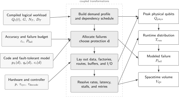
A resource estimate is a coupled dependency graph. The error budget selects protection; the scheduled demand selects factories and buffers; architecture constraints select routing and operation times. These choices jointly determine physical qubits, runtime, spacetime volume, and modeled failure.

Freeze the Estimation Contract

Before counting anything, state what success means. A minimal contract specifies:

• the problem instance and input distribution;
• the required numerical accuracy and confidence;
• whether cost is per attempt, per accepted sample, or per successful answer;
• the algorithm and all classical preprocessing and postprocessing;
• the allowed logical instruction set and synthesis policy;
• the code, decoder, fault-tolerant primitives, and layout;
• physical error, timing, leakage, loss, and correlation assumptions;
• the total failure budget and how it is allocated; and
• which outputs are peaks, averages, upper bounds, fitted projections, or simulated expectations.

Suppose one run succeeds with probability $P_{\mathrm{run}}$ and accepted runs require an average of $N_{\mathrm{rep}}$ algorithmic repetitions. If the whole job is restarted after a detected failure, the expected delivered cost is not the one-shot cost $C_{\mathrm{shot}}$ but approximately

$$\mathbb E[C_{\mathrm{delivered}}] = \frac{N_{\mathrm{rep}}C_{\mathrm{shot}}} {P_{\mathrm{run}}P_{\mathrm{accept}}}.$$

This simple denominator is often omitted. It matters whenever state preparation, postselection, heralded links, factory acceptance, or algorithmic sampling has nonunit success probability.

Logical Workload

Width and liveness

Let $q_\ell(t)$ be the number of logical qubits live at logical time $t$. The logical width relevant to hardware capacity is

$$Q_\ell^{\mathrm{peak}} = \max_t q_\ell(t),$$

not the number of named registers in source code and not necessarily the number of qubits in the problem Hamiltonian. Reversible arithmetic introduces ancillas; uncomputation releases them; measurement and reset may permit reuse. A compiler must therefore perform a liveness analysis or supply an equivalent schedule.

The width ledger should distinguish data, work, output, routing, and temporarily injected logical qubits:

$$Q_\ell^{\mathrm{peak}} = Q_{\mathrm{data}} +Q_{\mathrm{work}} +Q_{\mathrm{route}} +Q_{\mathrm{inject}} +Q_{\mathrm{I/O}}.$$

The terms need not peak simultaneously. Adding their independent maxima is a safe upper bound, but a time-resolved schedule can be substantially smaller.

Gate counts and dependency depth

For a declared logical gate alphabet $\mathcal G$, record a count vector

$$\mathbf N_{\mathcal G} = \left( N_{1q},N_{2q},N_{\mathrm{meas}},N_{\mathrm{reset}}, N_T,N_{CCZ},\ldots \right).$$

The alphabet matters. A Toffoli may be left as a native logical primitive, decomposed into Clifford+$T$, or supplied by a $|CCZ\rangle$ factory. Arbitrary rotations may be synthesized into $T$ gates, implemented by repeat-until- success gadgets, or realized through a code-specific analog primitive. Counts from different alphabets are not comparable until they are lowered to a common contract.

The compiled circuit is more faithfully represented by a directed acyclic graph $G=(V,E)$ than by a flat count. Each vertex is an operation with a duration and resource demand; edges carry quantum, classical, or feed-forward dependencies. A weighted critical path gives the idealized logical schedule length:

$$D_{\mathrm{crit}} = \max_{\pi\in\mathrm{paths}(G)} \sum_{v\in\pi} w(v).$$

This quantity changes after routing, factory allocation, measurement latencies, and classical reactions are inserted. It is therefore an input to, not the final answer from, the physical scheduler.

T count, T depth, and demand profile

In many surface-code architectures Clifford operations are relatively cheap while non-Clifford gates consume distilled resource states. Three summaries are useful:

$$N_T, \qquad D_T, \qquad \lambda_T(t).$$

$N_T$ is total demand, $D_T$ is the minimum number of causally sequential $T$ layers under a stated commutation and scheduling policy, and $\lambda_T(t)$ is the time-resolved number of states requested per scheduling interval. The first controls total production, the second lower-bounds reaction-limited time, and the third controls factory and buffer capacity.

A circuit with $(N_T,D_T)=(10^9,10^6)$ may request about $10^3$ simultaneous states in a typical active layer. Another circuit with the same pair may have bursty layers that request $10^6$ states followed by long Clifford regions. Only the demand profile distinguishes them.

Accuracy and Failure Budgets

Separate approximation from failure

Not every contribution to inaccuracy is a probability. It is useful to keep algorithmic and synthesis approximation errors separate from stochastic failure events:

$$\varepsilon_{\mathrm{tot}} \le \varepsilon_{\mathrm{alg}} +\varepsilon_{\mathrm{synth}} +\varepsilon_{\mathrm{model}} +\varepsilon_{\mathrm{stat}},$$ $$P_{\mathrm{fail}} \le P_{\mathrm{log}} +P_{\mathrm{dist}} +P_{\mathrm{inject}} +P_{\mathrm{read}} +P_{\mathrm{control}}.$$

The first line may use a norm, energy error, trace distance, or estimator bias, depending on the application. The second line is a conservative union bound over failure events. Adding the two lines is only justified after the application has supplied a common operational metric.

Allocate before solving for protection

For operation classes $i$ with counts $N_i$ and modeled logical failure per operation $p_i^{(L)}$, a first-order union bound gives

$$P_{\mathrm{log}} \le \sum_i N_i p_i^{(L)}.$$

Choose nonnegative allocations $\epsilon_i$ satisfying

$$\sum_i\epsilon_i \le \epsilon_{\mathrm{log}}, \qquad N_i p_i^{(L)} \le \epsilon_i.$$

Equal failure probability per operation is simple but seldom optimal. Memory, parity measurements, injections, distillation blocks, and long-range links can have different costs and logical-error laws. Resource minimization is an allocation problem:

$$\min_{\{d_i\}} R(\{d_i\}) \quad\text{subject to}\quad \sum_i N_i p_i^{(L)}(d_i) \le \epsilon_{\mathrm{log}}.$$

The integer variables $d_i$ make the result piecewise constant. Small changes in the target error may do nothing, then abruptly force a larger distance, another factory level, or an additional module.

Correlations and coherent errors

The union bound does not require independent failures, but the fitted $p_i^{(L)}$ model usually does depend on a noise class and decoder. A logical Pauli error rate fitted under independent depolarizing noise cannot simply be reused for coherent drift, leakage, erasure, spatial correlation, or burst noise. Common Noise Models explains these distinctions; Decoders explains why inference performance is part of the logical channel.

When coherent overrotations accumulate, amplitude-like bounds can scale as $N\theta$ while randomized stochastic contributions scale differently. A resource model must say whether twirling, randomized compiling, calibration, or a worst-case norm bound is assumed. Substituting average gate infidelity into a stochastic threshold fit is not generally valid.

Choosing Code Distance

A fitted suppression law

Below threshold, a common phenomenological model for a distance-$d$ surface code is

$$p_L(d,p) = A \left( \frac{p}{p_{\mathrm{th}}} \right)^{(d+1)/2},$$

where $p$ is a declared physical error parameter, $p_{\mathrm{th}}$ the threshold of the same circuit, noise, and decoder model, and $A$ a fitted prefactor. This is an architecture-specific empirical law, not the threshold theorem and not a universal identity.

If $N$ protected opportunities share a budget $\epsilon_L$, the sufficient condition $Np_L\le\epsilon_L$ yields

$$d \ge 2\, \frac{\ln(AN/\epsilon_L)} {\ln(p_{\mathrm{th}}/p)} -1.$$

The result must be rounded upward to a supported distance, often the next odd integer. The estimate should report the unrounded value, the chosen distance, and the fit’s calibration domain. Extrapolating a low-distance fit through many orders of magnitude can dominate the uncertainty of the entire result.

Distance is not always one number

A uniform distance is easy to communicate, but a machine may use different distances for data memory, lattice-surgery measurements, factories, output states, or network links. Asymmetric codes may use different $X$ and $Z$ distances. Bosonic inner codes may change the effective noise seen by an outer code. Quantum LDPC codes can replace a planar patch’s $O(d^2)$ geometric ledger with a different rate, check, connectivity, and decoder contract.

Thus the general object is a protection vector

$$\mathbf d = \left( d_{\mathrm{data}}, d_{\mathrm{op}}, d_{\mathrm{factory}}, d_{\mathrm{link}}, \ldots \right),$$

or, more generally, a list of code blocks and concatenation levels. The distance alone is insufficient without specifying what failure event it protects and for how many rounds.

Physical-Qubit Ledger

A credible peak inventory is additive at the architecture level:

$$Q_{\mathrm{phys}} = Q_{\mathrm{data}} +Q_{\mathrm{factory}} +Q_{\mathrm{route}} +Q_{\mathrm{buffer}} +Q_{\mathrm{I/O}} +Q_{\mathrm{spare}}.$$

The first term includes encoded data and work qubits. The remaining terms are not optional “overhead” in a runnable design: factories occupy hardware, states wait in buffers, patches or modules need communication space, and fabrication yield or disabled components may require spares.

For a patch-based surface-code model, write the physical footprint of patch class $a$ as

$$q_a(d) = \alpha_a d^2 +\beta_a d +\gamma_a.$$

Then a time-dependent layout has

$$Q_{\mathrm{phys}}(t) = \sum_a n_a(t)q_a(d_a) +Q_{\mathrm{fixed}}(t).$$

The familiar estimate “about $2d^2$ physical qubits per logical qubit” is one possible leading-order convention for a particular rotated layout and ancilla accounting. It is not a universal conversion factor. Boundaries, surgery lanes, unused tiles, measurement ancillas, defect margins, wiring constraints, and patch packing alter the coefficient.

For modular or photonic architectures, “physical qubit” may itself be a poor capacity unit. The ledger may need matter qubits per module, communication qubits, optical modes, sources, detectors, switches, link attempts, and buffering time. Report the native bottleneck quantities before collapsing them into a headline equivalent-qubit count.

Yield and availability

If a required component is independently usable with probability $y$, the mean number of fabricated components needed to obtain $Q$ usable components is $Q/y$. That mean does not set a high-confidence provision. For a fabricated capacity $Q_{\mathrm{fab}}$ and random usable count $X$, a yield-aware design instead chooses

$$\Pr(X\ge Q_{\mathrm{req}}) \ge 1-\epsilon_{\mathrm{yield}}.$$

Spatially correlated defects invalidate a binomial model. Whether defective sites can be routed around, and what that does to code distance and cycle time, belongs in the architecture assumptions.

Cycle Time and Operation Time

A physical gate time, a syndrome-extraction round, a code cycle, and a logical reaction time are different quantities. Let $\tau_{\mathrm{cyc}}$ denote the time for one complete repeated-error- correction round under a stated schedule. It includes the slowest required gate, measurement, reset, feed-forward, and synchronization stages, not just a representative two-qubit gate.

If logical operation $i$ occupies $c_i(\mathbf d)$ code cycles, its nominal duration is

$$t_i = c_i(\mathbf d)\tau_{\mathrm{cyc}}.$$

For lattice surgery, protected parity measurements commonly require a number of rounds proportional to distance, followed by decoding and any conditional frame update. A more complete reaction duration is

$$t_{\mathrm{react}} = c_{\mathrm{meas}}\tau_{\mathrm{cyc}} +\tau_{\mathrm{decode}} +\tau_{\mathrm{comm}} +\tau_{\mathrm{control}}.$$

Pauli-frame updates may be tracked in software without an immediate physical gate, but a later non-Clifford choice can depend on the decoded result. At that point classical latency lies on the quantum critical path. Decoder throughput must also keep pace with syndrome production; low average latency is not enough if queues grow without bound.

Magic-State Factories

Quality, rate, footprint, and acceptance

A factory model needs at least four outputs:

$$\left( p_{\mathrm{out}}, b, \tau_F, q_F \right),$$

where $p_{\mathrm{out}}$ is the output error, $b$ the number of usable states per accepted batch, $\tau_F$ the batch period, and $q_F$ the physical footprint. If the batch is accepted with probability $a$, the mean production rate of one factory is

$$\mu_F = \frac{ab}{\tau_F}.$$

The distillation error budget requires, for example,

$$N_T p_{\mathrm{out}} \le \epsilon_{\mathrm{dist}},$$

with additional terms for injection, storage, transport, and correlated factory failures. A protocol’s algebraic suppression order alone does not specify these quantities; circuit-level faults, code distance, acceptance, and layout must be included.

Supply must match a scheduled demand

For $M$ identical factories, the average-rate condition

$$M\mu_F \ge \overline{\lambda_T}$$

is necessary for a steady workload but not sufficient for a bursty one. Let $S_k$ be states supplied and $C_k$ states consumed during scheduling interval $k$. A buffer of capacity $B_{\max}$ evolves as

$$B_{k+1} = \min \left[ B_{\max}, B_k+S_k-C_k \right],$$

subject to $B_k+S_k\ge C_k$ whenever the data path is not allowed to stall. State aging, storage errors, and routing occupancy can limit how large $B_{\max}$ should be.

Factories therefore create a space–time tradeoff. More factories consume qubits and may reduce runtime; fewer factories save area but can serialize the non-Clifford path. Factory failures add randomness, so a high-confidence schedule may need spare capacity, a buffer, or a quantified stall probability. Sizing from mean throughput alone silently assumes away this tail risk.

Multiple resource-state species

An architecture may consume $|T\rangle$, $|CCZ\rangle$, arbitrary-angle states, Bell pairs, or encoded resource states at different fidelities. Then the supply problem is vector-valued:

$$\boldsymbol\lambda(t) = \left( \lambda_T(t), \lambda_{CCZ}(t), \lambda_{\theta}(t), \lambda_{\mathrm{Bell}}(t), \ldots \right).$$

Conversions between species have loss, latency, and footprint. A single “magic-state count” can hide the dominant factory or network bottleneck.

Runtime and Scheduling

Lower bounds

Several independent bottlenecks give useful runtime lower bounds. If the scheduled protected circuit has duration $D_{\mathrm{sched}}$ in its base time unit, $M$ factories each supply at rate $\mu_F$, and the workload needs $N_T$ states, then

$$T_{\mathrm{run}} \ge \max \left( D_{\mathrm{sched}}\tau_{\mathrm{unit}}, \frac{N_T}{M\mu_F}, T_{\mathrm{classical}}, T_{\mathrm{I/O}} \right).$$

This maximum is a diagnostic, not a complete scheduler. Routing conflicts, factory bursts, shared ancillas, module links, measurement dependencies, and maintenance windows couple the terms. A feasible schedule must assign every operation an interval and every occupied resource a location without violating dependencies or capacity.

Throughput-limited and reaction-limited regimes

Two limiting cases are especially useful:

• In a throughput-limited regime, non-Clifford states or entangled links are consumed as quickly as they can be produced. Adding factories or links reduces runtime until another bottleneck takes over.
• In a reaction-limited regime, the critical path repeatedly waits for a logical measurement, decoding, classical communication, and a conditional operation. Extra factories do not remove that serial latency.

The distinction explains why $T$ count can predict runtime well for one architecture while $T$ depth or classical reaction depth predicts it for another.

Expected runtime

If one scheduled attempt takes $T_{\mathrm{shot}}$, succeeds with probability $P_{\mathrm{run}}$, and independent restarts are allowed, then

$$\mathbb E[T_{\mathrm{success}}] = \frac{T_{\mathrm{shot}}}{P_{\mathrm{run}}}.$$

The time to achieve confidence $1-\delta$ may be more relevant than the mean. For independent attempts with success probability $P_{\mathrm{run}}$, the smallest number of attempts satisfying that confidence is

$$n_{\delta} = \left\lceil \frac{\ln\delta} {\ln(1-P_{\mathrm{run}})} \right\rceil.$$

Report both when the distribution has operational significance.

Spacetime Volume

Peak qubits and runtime are projections of a time-dependent occupancy. Its integral is the physical spacetime volume

$$V_{Q t} = \int_0^{T_{\mathrm{run}}} Q_{\mathrm{active}}(t)\,dt.$$

For a code-cycle schedule,

$$V_{Q c} = \sum_k Q_k\Delta c_k$$

is measured in physical-qubit-cycles. Logical block-cycles, patch-cycles, or tile-cycles are useful intermediate units only when their conversion is declared.

Spacetime volume captures a real tradeoff: doubling hardware to halve time can leave $V_{Qt}$ approximately unchanged. It is also a rough exposure measure for local stochastic faults. It is not a complete cost function, because control electronics, energy, fabrication, network use, and idle hardware need not scale with active qubit-seconds.

Architecture Assumptions

No physical estimate is meaningful without an architecture sheet. At minimum it should specify the following.

Code and logical operations

• code family, boundary conditions, supported distances, and decoder;
• logical gate set and realization of each primitive;
• syndrome-extraction circuit and number of rounds per operation;
• whether distance changes, gauge fixing, transversal gates, surgery, or teleportation are allowed; and
• distillation protocols, injection model, factory placement, and buffers.

Hardware and noise

• native operations, connectivity, parallelism, and conflict rules;
• gate, measurement, reset, transport, and entanglement-generation times;
• error channels, leakage, erasure or loss, crosstalk, drift, and correlations;
• calibration and maintenance assumptions; and
• fabrication yield, disabled-component tolerance, and spare policy.

Classical system

• syndrome bandwidth and where data are aggregated;
• decoder accuracy, throughput, latency distribution, and backlog policy;
• controller and interconnect latency;
• conditional-branch and Pauli-frame handling; and
• memory, compute, and power provision for the classical path.

Facility and modularity

• module capacity, link topology, Bell-pair rate and fidelity;
• purification, heralding, retry, and timeout policies;
• cryogenic wiring, optical switching, or control-channel constraints; and
• which components can operate concurrently.

These assumptions should be machine-readable where possible, but prose is still needed to state exclusions. “All-to-all connectivity” might mean native two-qubit gates, teleportation through a shared bus, or a compiler abstraction whose physical cost has not yet been modeled.

Worked Example: Distance, Factories, and Runtime

Consider a deliberately simplified logical workload with

$$Q_\ell^{\mathrm{peak}}=100, \qquad N_{\mathrm{opp}}=10^{10}, \qquad N_T=10^8, \qquad D_T=2\times10^6.$$

Allocate $\epsilon_{\mathrm{log}}=10^{-2}$ to protected logical opportunities. Suppose a calibrated model uses

$$p_L(d) = 0.1(0.1)^{(d+1)/2}.$$

The condition $N_{\mathrm{opp}}p_L(d)\le10^{-2}$ becomes

$$10^{10}\times0.1\times10^{-(d+1)/2} \le10^{-2},$$

so $(d+1)/2\ge11$ and the smallest supported odd distance is $d=21$. This conclusion is conditional on the fitted law; it is not inferred from the physical error rate alone.

Assume each of 140 simultaneously occupied data, work, and routing patches uses $2d^2$ physical qubits under the chosen layout convention. Their nominal footprint is

$$Q_{\mathrm{core}} = 140\times2\times21^2 =123{,}480.$$

Now suppose one factory occupies $50{,}000$ physical qubits and emits one accepted $T$ state every $50\,\mu\mathrm{s}$ on average. Its rate is $\mu_F=2\times10^4\,\mathrm{s}^{-1}$. Four factories supply $8\times10^4\,\mathrm{s}^{-1}$, giving the throughput lower bound

$$T_T \ge \frac{10^8}{8\times10^4\,\mathrm{s}^{-1}} =1250\,\mathrm{s}.$$

If one adaptive $T$ layer takes $20\,\mu\mathrm{s}$, the reaction-depth bound is

$$T_{D_T} \ge 2\times10^6\times20\,\mu\mathrm{s} =40\,\mathrm{s}.$$

This scenario is factory-throughput limited, with a nominal peak inventory

$$Q_{\mathrm{phys}} \ge 123{,}480 +4\times50{,}000 =323{,}480,$$

before buffers, injection patches, I/O, spares, and controller constraints. Increasing to 40 factories would lower the production bound to $125$ s but raise the nominal inventory above two million physical qubits. At some point routing or reaction depth becomes limiting. The example’s value is not its headline number; it is the visible chain of assumptions that lets another reader replace any term.

Sensitivity, Scenarios, and Discrete Jumps

For a smooth output $R$ and input $x$, a local logarithmic sensitivity is

$$S_x = \frac{\partial\ln R}{\partial\ln x}.$$

This can identify influential continuous inputs such as cycle time or factory period. Fault-tolerant estimates are not globally smooth, however. Distance rounding, factory count, module count, and layout feasibility create steps. A local derivative taken inside one plateau can therefore report zero even though the next small change crosses a costly boundary.

Use at least three declared scenarios when inputs are projections rather than measurements: conservative, central, and optimistic. Recompute the entire model in each scenario instead of scaling the final answer. A faster cycle may change runtime directly, permit a different schedule, alter decoder backlog, and change the memory failure budget. Correlated inputs should be varied together when they come from one technology assumption.

The software workflow for parameter sweeps, uncertainty distributions, versioning, and reproducibility belongs to Resource Estimation Tools.

How to Audit an Estimate

Use the following order because each step depends on the preceding contract.

1. Identify the task. Record instance size, output accuracy, confidence, and whether costs are per shot or per successful result.
2. Inspect the logical artifact. Verify gate semantics, ancilla liveness, count vector, dependency graph, approximation policy, and repetitions.
3. Check the error ledger. Confirm that all failure and approximation sources are named, allocated, and expressed in compatible metrics.
4. Recompute protection. Evaluate the logical-error model, rounding rule, operation count, distance choices, and extrapolation range.
5. Rebuild the qubit inventory. Sum core, factory, route, buffer, I/O, and spare terms; do not accept a bare qubits-per-logical-qubit multiplier.
6. Check rates and peaks. Compare the time-resolved consumption of every scarce state or link with production, acceptance, buffering, and routing.
7. Trace the critical path. Include code cycles, measurement, decoding, communication, control, retries, and classical preprocessing.
8. Recompute success cost. Convert one-shot resources to delivered-answer resources using acceptance and restart probabilities.
9. Stress the assumptions. Vary the parameters that choose distance, factory count, layout, and bottleneck regime.
10. Demand provenance. Require code, data, versions, seeds where relevant, and enough intermediate outputs to reproduce every conversion.

An estimate that exposes only final qubits and seconds cannot pass this audit, even if those numbers happen to be close to a later design.

Common Mistakes

Treating asymptotic scaling as an engineering estimate

A statement such as $O(n^3)$ gates suppresses constants, ancillary width, precision dependence, success amplification, gate types, and architecture. It can compare algorithm families but cannot size a machine.

Multiplying logical width by a universal patch factor

The core data block is only one part of the inventory. Factories, routing, buffers, I/O, dead space, and spares can dominate. Even the patch coefficient depends on layout conventions.

Using one error rate everywhere

Gate infidelity, measurement error, erasure, leakage, logical failure per round, and diamond-norm error are different quantities. A threshold fit is valid only for its stated circuit, noise, and decoder model.

Converting T count directly to time

Runtime depends on factory throughput, burstiness, $T$ depth, routing, and reaction latency. The quotient $N_T/\mu_F$ is a lower bound only after the number and acceptance of factories are fixed.

Ignoring classical control

Syndrome decoding can be throughput-limited, while adaptive operations can be latency-limited. A controller that eventually produces the correct answer may still be too slow to prevent backlog or memory exposure.

Reporting false precision

An integer output from software is exact relative to its internal inputs. It does not make projected physical error rates, fitted extrapolations, or future cycle times exact. Report sensitivity and provenance rather than decorative significant figures.

Comparing incomparable headlines

Two qubit counts may target different success probabilities, logical gate sets, cycle times, layouts, or output accuracy. Normalize the contract before ranking them.

Exercises

1. Distance from a logical-error budget

A workload has $N=10^9$ protected opportunities and budget $\epsilon_L=10^{-3}$. Its fitted logical error per opportunity is $p_L(d)=0.05(0.08)^{(d+1)/2}$. Find the smallest supported odd distance.

Solution

Require

$$10^9\times0.05\times(0.08)^{(d+1)/2} \le10^{-3}.$$

Taking logarithms gives

$$\frac{d+1}{2} \ge \frac{\ln(10^{-3}/(5\times10^7))}{\ln(0.08)} \approx9.75.$$

Thus $d\ge18.5$. Rounding upward to a supported odd distance gives $d=19$. Substitution is the final check: $10^9(0.05)(0.08)^{10}\approx5.37\times10^{-4}$, which is within budget.

2. T count is not runtime

Two compiled circuits each have $N_T=10^6$ and $D_T=10^4$. Circuit A requests 100 states in each active layer. Circuit B alternates layers requesting 1 and 199 states. A factory bank can deliver 120 states per layer and the buffer is empty initially. Which circuit can run without stalls under that schedule?

Solution

Circuit A consumes 100 states per active layer, below the supply of 120, so it does not stall and accumulates a surplus if storage is available. Circuit B’s 199-state layers cannot be served from an initially empty buffer after only one 120-state production interval. Its average demand can match A’s, but its peak demand violates capacity. A warm-up interval or buffer fed during the preceding one-state layer could remove later stalls. The example shows why $(N_T,D_T)$ does not determine feasibility without $\lambda_T(t)$ and an initial-buffer policy.

3. Optimize a two-class error allocation

Memory has $N_m=10^8$ opportunities with cost $q_m(d_m)=d_m^2$; surgery has $N_s=10^6$ opportunities with cost $q_s(d_s)=20d_s^2$. Both use $p_L(d)=10^{-(d+1)/2}$. Explain why assigning equal error per opportunity need not minimize total cost under $N_mp_L(d_m)+N_sp_L(d_s)\le10^{-3}$.

Solution

Equal error per opportunity imposes $p_L(d_m)=p_L(d_s)$ and therefore equal distances. But increasing $d_s$ is twenty times more expensive per protected object, while there are one hundred times fewer surgery opportunities. It can be cheaper to assign a larger fraction of the failure budget to surgery and protect memory more strongly. The exact optimum is discrete: enumerate the supported odd pairs $(d_m,d_s)$, discard infeasible pairs, and minimize the declared combined footprint or spacetime objective. Error allocation is an optimization variable, not a fairness rule.

4. Physical-qubit inventory

An architecture uses 300 data patches of $2d^2$ qubits at $d=25$, six factories of $80{,}000$ qubits, 90 routing patches of the same data-patch size, a buffer of 40 patches, and a 12% spare margin applied after summing those components. Compute the provisioned peak.

Solution

One patch uses $2(25)^2=1250$ physical qubits. Data, routing, and buffer use

$$(300+90+40)1250 =537{,}500.$$

Factories use $6(80{,}000)=480{,}000$, so the pre-spare total is $1{,}017{,}500$. Applying the declared margin gives

$$Q_{\mathrm{provisioned}} = \left\lceil1.12\times1{,}017{,}500\right\rceil =1{,}139{,}600.$$

The calculation is auditable because the margin’s scope is explicit.

5. Factory count and bottleneck transition

A computation needs $N_T=3\times10^9$ states. Each factory produces an accepted state every $40\,\mu\mathrm{s}$. The nonfactory critical path is $10^4$ s. Find the smallest factory count for which average state production is no longer the runtime lower bound.

Solution

One factory has rate $\mu_F=25{,}000\,\mathrm{s}^{-1}$. Require

$$\frac{3\times10^9}{M(25{,}000\,\mathrm{s}^{-1})} \le10^4\,\mathrm{s},$$

which gives $M\ge12$. At 12 factories, the production bound equals $10^4$ s. This is only an average-rate result; burst demand, acceptance variance, routing, and buffers may require more factories.

6. Expected versus high-confidence attempts

One run lasts 6 hours and succeeds with probability $0.8$. Find the expected time to a successful run and the number of complete attempts needed for at least 99% probability of one success.

Solution

The expected time is $6/0.8=7.5$ hours. For confidence $0.99$, require $(1-0.8)^n\le0.01$, so

$$n \ge \frac{\ln0.01}{\ln0.2} \approx2.86.$$

Three attempts suffice, corresponding to an 18-hour worst-case reservation under this simple complete-restart policy. Expected and reserved resources answer different operational questions.

7. Cycle-time audit

A report quotes a 20 ns two-qubit gate and infers a 20 ns code cycle. The syndrome circuit actually has four sequential two-qubit layers, 100 ns measurement, 80 ns reset, and 40 ns synchronization. Assuming those stages are sequential, compute the cycle time and the error in the quoted value.

Solution

The complete cycle is

$$\tau_{\mathrm{cyc}} = 4(20\,\mathrm{ns}) +100\,\mathrm{ns} +80\,\mathrm{ns} +40\,\mathrm{ns} =300\,\mathrm{ns}.$$

The quoted value is too small by a factor of 15. A real schedule may overlap some stages, but that overlap must be demonstrated rather than assumed.

8. Design an audit record

List the minimum intermediate outputs needed to make a published estimate of physical qubits and runtime independently checkable.

Solution

A defensible record includes the problem instance and success criterion; logical circuit or call graph; logical width and liveness; counts by gate and state species; dependency or reaction depth; synthesis errors; complete failure-budget allocation; logical-error models and fitted domains; chosen distances and rounding; patch or block inventory; factory protocols, acceptance, rate, and footprint; routing and buffer policy; cycle and reaction times; schedule or bottleneck evidence; retry model; architecture and noise parameters; software and data versions; and final qubits, runtime, spacetime, and modeled failure probability. The Reporting Standards page develops the publication-level provenance record.

Research Status

The accounting identities on this page are standard. The numerical models inserted into them remain active research. Algorithmic decompositions, rotation synthesis, code families, decoders, lattice-surgery layouts, distillation and cultivation protocols, modular links, classical controllers, and hardware error models continue to improve. Published end-to-end estimates are therefore conditional snapshots, not timetables.

Evidence strength also varies by layer. A logical gate count may be verified exactly from a compiler artifact; a code-distance fit may come from circuit-level Monte Carlo simulation over a limited range; a projected million-qubit cycle time may be an engineering target; and a useful application runtime may depend on an unvalidated input-state assumption. A single table should not present these as equally observed facts.

Current resource estimation is strongest when it exposes the complete chain, reports alternatives, and identifies the bottleneck regime. Its most durable result is often not the final integer but the finding that, under a declared contract, runtime is controlled by reaction depth, magic-state throughput, communication, or another specific subsystem.

Further Connections

• Threshold Theorem explains why scalable suppression is possible and why theorem thresholds do not supply universal engineering parameters.
• Fault-Tolerant Gates defines the error-containment gadgets whose durations and failure locations populate the model.
• Surface Code supplies planar-code geometry, repeated checks, logical operations, and calibrated suppression laws.
• Magic-State Distillation develops output-error polynomials, acceptance, protocol levels, and factory constructions.
• Lattice Surgery supplies protected parity operations, routing lanes, patch occupancy, and schedule constraints.
• Quantum LDPC Codes shows why rate, check connectivity, decoder complexity, and logical operations must replace a surface-code patch multiplier in other code families.
• Logical Benchmarking supplies measured logical failure, timing, acceptance, throughput, and footprint inputs for the cost model.
• Resource Estimation Tools turns this cost model into a reproducible software and analysis workflow.
• Metrics for Quantum Hardware defines the measured operation, timing, leakage, crosstalk, throughput, and logical quantities supplied as hardware inputs.
• Shor Algorithm is a canonical example in which arithmetic design, retry probability, factory throughput, and reaction time all move the final estimate.
• Quantum Phase Estimation connects target precision, coherent evolution, input overlap, repetitions, and fault-tolerant cost.
• Error-Correction Case Studies distinguishes demonstrated logical suppression from projected application-scale resources.
• Fault-Tolerant Quantum Computing Frontier places resource reductions beside experimental and architectural evidence.

References

1. M. E. Beverland et al., “Assessing requirements to scale to practical quantum advantage,” arXiv:2211.07629 (2022), arXiv:2211.07629.
2. A. G. Fowler, M. Mariantoni, J. M. Martinis, and A. N. Cleland, “Surface codes: Towards practical large-scale quantum computation,” Physical Review A 86, 032324 (2012), doi:10.1103/PhysRevA.86.032324.
3. D. Litinski, “A game of surface codes: Large-scale quantum computing with lattice surgery,” Quantum 3, 128 (2019), doi:10.22331/q-2019-03-05-128.
4. C. Gidney and A. G. Fowler, “Efficient magic state factories with a catalyzed $|CCZ\rangle$ to $2|T\rangle$ transformation,” Quantum 3, 135 (2019), doi:10.22331/q-2019-04-30-135.
5. C. Gidney and M. Ekerå, “How to factor 2048 bit RSA integers in 8 hours using 20 million noisy qubits,” Quantum 5, 433 (2021), doi:10.22331/q-2021-04-15-433.
6. M. Reiher, N. Wiebe, K. M. Svore, D. Wecker, and M. Troyer, “Elucidating reaction mechanisms on quantum computers,” Proceedings of the National Academy of Sciences 114, 7555–7560 (2017), doi:10.1073/pnas.1619152114.
7. V. von Burg et al., “Quantum computing enhanced computational catalysis,” Physical Review Research 3, 033055 (2021), doi:10.1103/PhysRevResearch.3.033055.
8. N. J. Ross and P. Selinger, “Optimal ancilla-free Clifford+$T$ approximation of $z$-rotations,” Quantum Information and Computation 16, 901–953 (2016), arXiv:1403.2975.
9. A. G. Fowler, A. C. Whiteside, and L. C. L. Hollenberg, “Towards practical classical processing for the surface code,” Physical Review Letters 108, 180501 (2012), doi:10.1103/PhysRevLett.108.180501.
10. Y. Kurman et al., “Controller-decoder system requirements derived by implementing Shor’s algorithm with surface code,” Quantum 10, 2170 (2026), doi:10.22331/q-2026-07-22-2170.
11. A. Paetznick and B. W. Reichardt, “Universal fault-tolerant quantum computation with only transversal gates and error correction,” Physical Review Letters 111, 090505 (2013), doi:10.1103/PhysRevLett.111.090505.
12. S. Bravyi and A. Kitaev, “Universal quantum computation with ideal Clifford gates and noisy ancillas,” Physical Review A 71, 022316 (2005), doi:10.1103/PhysRevA.71.022316.
13. E. T. Campbell, B. M. Terhal, and C. Vuillot, “Roads towards fault-tolerant universal quantum computation,” Nature 549, 172–179 (2017), doi:10.1038/nature23460.
14. A. G. Fowler, “Time-optimal quantum computation,” arXiv:1210.4626 (2012), arXiv:1210.4626.
15. M. P. Harrigan et al., “Expressing and analyzing quantum algorithms with Qualtran,” arXiv:2409.04643 (2024), arXiv:2409.04643.
16. A. W. Cross et al., “OpenQASM 3: A broader and deeper quantum assembly language,” ACM Transactions on Quantum Computing 3, article 12 (2022), doi:10.1145/3505636.
17. M. A. Nielsen and I. L. Chuang, Quantum Computation and Quantum Information, 10th anniversary ed., Cambridge University Press (2010), doi:10.1017/CBO9780511976667.