Syndrome Measurement

A syndrome measurement is a physical instrument that extracts the eigenvalue of a declared Pauli check while preserving the unresolved quantum information inside each eigenspace. This page derives the ideal two-branch instrument, implements Z- and X-type products with an ancilla, distinguishes raw readout bits from signed syndrome bits, and turns repeated outcomes into boundary-aware detector parities. An ordered four-body audit then shows exactly what six single faults do and do not establish. The scope is code independent: it ends at a reproducible extraction record, before decoder inference, code-specific schedules, or a proof that an entire error-correction gadget is fault tolerant.

Required background. Multi-Qubit Gates supplies CNOT action, generic parity instruments, and elementary data–ancilla circuits. Stabilizer Formalism supplies stabilizer groups, syndrome algebra, projectors, normalizers, logical cosets, and ideal Pauli-measurement updates.

Helpful background. Pauli Group and Stabilizers develops phase-safe signed checks and algebraic commutation signatures. The Quantum Error Correction and Fault Tolerance guide places physical extraction between code algebra and decoder or gadget analysis.

Check Measurements as Lüders Instruments

The mathematical input is a finite-qubit signed Pauli check $g$ that is a Hermitian involution,

$$g=g^\dagger, \qquad g^2=I.$$

These conditions, rather than the word Pauli alone, make $g$ a binary observable. A phase-rich Pauli-group element such as $iP$ or $-iP$ is anti-Hermitian when $P$ is Hermitian and is not a $\pm1$-valued check. Retaining the sign is equally important: $P$ and $-P$ have the same eigenspaces but exchange which one is labeled $+1$.

Hermitian involutions define two eigenspaces

Encode the observed eigenvalue by a bit $b\in\{0,1\}$ through $\lambda_b=(-1)^b$. The two spectral projectors are

$$\Pi_b = \frac{I+(-1)^b g}{2}.$$

Hermiticity of $g$ makes each $\Pi_b$ Hermitian, and $g^2=I$ gives

$$\Pi_b^2=\Pi_b, \qquad \Pi_0\Pi_1=0, \qquad \Pi_0+\Pi_1=I.$$

Thus $b=0$ names the $+1$ eigenspace and $b=1$ names the $-1$ eigenspace. This convention must be written into the extraction contract: some software and experimental records instead store an eigenvalue, a sign, or an inverted hardware discriminator. None is intrinsically wrong, but an unstated conversion can reverse every syndrome.

Quantity	Definition	Identity or normalization	Operational meaning
Signed check $g$	$g=g^\dagger$ and $g^2=I$	spectrum contained in $\{+1,-1\}$	binary observable whose sign is part of the specification
Projector $\Pi_b$	$[I+(-1)^b g]/2$	$\Pi_b^2=\Pi_b$ and $\Pi_0+\Pi_1=I$	selects the eigenspace labeled by bit $b$
Selected branch $\mathcal I_b(\rho)$	$\Pi_b\rho\Pi_b$	positive and generally subnormalized	unnormalized state associated with recorded outcome $b$
Probability $p_b$	$\operatorname{Tr}[\mathcal I_b(\rho)]$	$p_b\geq0$ and $p_0+p_1=1$	Born probability of branch $b$ for normalized $\rho$
Unread map $\sum_b\mathcal I_b$	$\sum_b\Pi_b\rho\Pi_b$	completely positive and trace preserving	state after the check when its classical outcome is discarded

Ideal branch maps retain Born weights

The outcome-resolved state transformation used here is

$$\mathcal I_b(\rho) = \Pi_b\rho\Pi_b, \qquad p_b = \operatorname{Tr}[\mathcal I_b(\rho)].$$

The family $\{\mathcal I_0,\mathcal I_1\}$ is the subnormalized ideal Lüders instrument. The trace of a selected branch is deliberately retained; normalizing first would erase its outcome probability. Only when $p_b>0$ is the conditional state defined:

$$\rho_{\mid b} = \frac{\mathcal I_b(\rho)}{p_b}.$$

If the outcome is unread, the relevant channel is $\sum_b\mathcal I_b$. It preserves blocks within either eigenspace and removes coherence between the two eigenspaces. Gottesman’s stabilizer treatment supplies the projector and Pauli-update foundations used here, while Terhal’s review places repeated stabilizer measurement in the larger error-correction workflow.

The observable $g$ fixes its projectors and outcome probabilities, but it does not uniquely fix every possible disturbance. A device could apply an outcome-dependent unitary within an eigenspace, leak population, or realize a finer measurement and then coarse-grain its record. Calling the map Lüders is therefore a physical idealization, not a consequence of merely naming $g$. The general classification of such alternatives belongs to Quantum Instruments.

Logical opacity requires a stabilizer premise

Suppose a code space $\mathcal C$ is stabilized by $g$, so $g\lvert\psi_L\rangle=\lvert\psi_L\rangle$ for every encoded state $\lvert\psi_L\rangle\in\mathcal C$. For a fixed Pauli error $E$,

$$gE\lvert\psi_L\rangle = \begin{cases} +E\lvert\psi_L\rangle, & [E,g]=0,\\ -E\lvert\psi_L\rangle, & \{E,g\}=0. \end{cases}$$

The check outcome records the commutation sign of $E$ with $g$. It does not distinguish the amplitudes of $\lvert\psi_L\rangle$ because $g$ acts as the same scalar on the whole code space. This is the precise sense in which a stabilizer syndrome can be learned without reading out logical information.

The premise cannot be weakened to “$g$ commutes with the stabilizer.” A Pauli in the normalizer but outside the stabilizer can be a logical observable. Measuring it may reveal an encoded eigenvalue and dephase a logical superposition. Likewise, a coherent error that populates several syndrome sectors is dephased by the unread Lüders channel even though coherence within each degenerate sector is preserved. Finally, measuring every data qubit in a product basis and XORing the results may furnish a terminal parity, but the fine-grained outcomes reveal more information and destructively alter the data. That procedure is not the same nondemolition instrument.

For a density operator, the same boundary is visible without choosing an encoded basis. Decompose $\rho$ into blocks $\Pi_b\rho\Pi_{b'}$. The unread instrument retains the two diagonal blocks and deletes the $b\ne b'$ blocks. If the state is already supported in one stabilizer sector, the ideal check leaves it unchanged; if an incoherent mixture occupies both sectors, the outcome updates their classical weights; if a coherent process connects them, unread extraction destroys that intersector phase. None of these statements says that the apparatus is quantum nondemolition under repeated hardware use: reset error, leakage, relaxation, and unmodeled couplings require separate evidence.

Ancilla Circuits for Z- and X-Type Checks

An ancilla converts a many-qubit parity into one pointer degree of freedom. The circuit must preserve the degeneracy of the check: basis states with the same parity lead to the same ancilla pointer, rather than to distinguishable records for each data string. A fresh ancilla, a declared CNOT orientation, and a matching readout basis make this coarse measurement explicit.

Check family	Ancilla preparation	CNOT orientation	Ancilla readout	Indirect pointer states
Z-type product	fresh $\lvert0\rangle_a$	each data qubit is control; ancilla is target	Z basis	$\lvert0\rangle_a,\lvert1\rangle_a$
X-type product	fresh $\lvert+\rangle_a$	ancilla is control; each data qubit is target	X basis	$\lvert+\rangle_a,\lvert-\rangle_a$

A target ancilla accumulates Z parity

For $P_Z=\prod_{j\in S}Z_j$, prepare $\lvert0\rangle_a$ and apply $\operatorname{CNOT}_{j\to a}$ for each $j\in S$. On a computational-basis string $\lvert x\rangle$ the ancilla becomes

$$\lvert x\rangle\lvert0\rangle_a \longmapsto \lvert x\rangle \left\lvert\bigoplus_{j\in S}x_j\right\rangle_a.$$

Even strings point to $\lvert0\rangle_a$ and odd strings to $\lvert1\rangle_a$, precisely the $+1$ and $-1$ eigenspaces of $P_Z$. By linearity, a superposition inside either parity sector remains coherent because every component in that sector produces the same pointer state. Measuring the ancilla in Z therefore realizes the ideal projectors on the data in the fault-free model; it does not reveal which computational string occurred.

Writing an arbitrary input as $\lvert\psi\rangle=\Pi_0\lvert\psi\rangle+\Pi_1\lvert\psi\rangle$ makes the coarse action explicit. After the interactions the joint state is

$$\Pi_0\lvert\psi\rangle\lvert0\rangle_a + \Pi_1\lvert\psi\rangle\lvert1\rangle_a.$$

Projecting the ancilla onto $\lvert b\rangle_a$ leaves the unnormalized data vector $\Pi_b\lvert\psi\rangle$; the density-operator branch is therefore $\Pi_b\rho\Pi_b$. This derivation proves the fault-free unsigned circuit action. A negative sign in $g$ does not require changing these gates: it changes the classical mapping from the circuit’s pointer bit to the stored signed bit.

The ancilla must be fresh or demonstrably reset. An unknown prior $X_a$ changes the recorded parity, while entanglement with an earlier round can correlate nominally separate records. Preparation, reset, and measurement are operations in the protocol, not invisible punctuation around the CNOT sequence.

A control ancilla accumulates X parity

For $P_X=\prod_{j\in S}X_j$, prepare $\lvert+\rangle_a$, use the ancilla as the control of every $\operatorname{CNOT}_{a\to j}$, and measure it in the X basis. If $\lvert\phi_\lambda\rangle$ is an eigenstate of $P_X$ with eigenvalue $\lambda\in\{+1,-1\}$, then the controlled product gives

$$\frac{ \lvert0\rangle_a\lvert\phi_\lambda\rangle + \lvert1\rangle_a P_X\lvert\phi_\lambda\rangle }{\sqrt2} = \begin{cases} \lvert+\rangle_a\lvert\phi_\lambda\rangle, & \lambda=+1,\\ \lvert-\rangle_a\lvert\phi_\lambda\rangle, & \lambda=-1. \end{cases}$$

The pointer states are now $\lvert+\rangle_a$ and $\lvert-\rangle_a$. Reading the ancilla in X distinguishes the product eigenvalue without resolving the individual data qubits. This circuit is the Hadamard-dual of Z-parity extraction, but its fault-propagation asymmetry is also dual: changing which wire is the control changes which ancilla Pauli can fan out.

Local basis changes extend the pointer construction

A mixed Pauli product such as $X_1Y_2Z_4$ can be reduced to a Z-type product by declared one-qubit basis changes before the parity interaction and their inverses afterward. For example, $H$ maps X to Z, while a suitable Clifford combination maps Y to Z. An equivalent implementation may use controlled-Pauli gates directly. Either description must state the gate convention and order, because those extra operations add fault locations and can change propagation.

The ideal projector depends only on the final signed product, but the physical circuit does not. Two circuits that measure the same $g$ in the absence of faults can respond differently to an ancilla error inserted halfway through. This distinction is why an extraction method needs both an operator specification and an ordered implementation record.

Basis changes also constrain what “the same fault” means. A physical Z fault placed before an $H$ can become X afterward, and a fault during the basis-change gate need not be a single Pauli in a microscopic model. A Pauli ledger is exact for its declared inserted Pauli faults and a useful component of stochastic Pauli models; it is not automatically a complete device-noise characterization.

Signed Outcomes and the Extraction Contract

A practical record usually begins with an unsigned circuit for a phase-free product $P$. Stabilizer generators, frames, and calibration conventions may instead demand the signed check $g=(-1)^\sigma P$. The circuit discriminator, sign offset, stored syndrome, and eigenvalue must remain separate objects.

Raw circuit bits are not signed syndrome bits

Let the circuit report raw bit $r$, where $r=0$ means eigenvalue $+1$ for $P$ and $r=1$ means eigenvalue $-1$. For $\sigma\in\{0,1\}$ define

$$g=(-1)^\sigma P, \qquad m=r\oplus\sigma,$$

so that

$$\lambda_P=(-1)^r, \qquad \lambda_g=(-1)^m.$$

If $g=-P$, then $\sigma=1$: a raw $r=0$ is correctly stored as $m=1$, because the state with $P$ eigenvalue $+1$ has $g$ eigenvalue $-1$. The offset can also absorb a documented frame or circuit convention, but every such contribution must be reproducible. Silently overwriting $r$ with $m$ makes later diagnosis impossible: one can no longer tell whether an unexpected bit came from physical readout, an intentional sign, or a classical conversion.

The word syndrome is used at several resolutions. Here $m$ is one signed check outcome. A round’s syndrome is a vector of such outcomes for a declared check set. A detector is a parity among outcomes expected to vanish in the no-fault model. A decoder then uses many detector values and a noise model to infer a correction or frame update. These objects are related, but none is interchangeable with the next.

A reproducible protocol fixes support, order, resets, and readout

An extraction contract identifies the signed check and its ordered support; the physical ancilla; its preparation and reset; every gate’s orientation and chronological order; the measurement basis; and the raw-outcome convention. For repeated extraction it must also state the round cadence, classical sign or frame offsets, allowed fault locations, treatment of missing or invalid telemetry, and the initial and terminal relations that close the detector record.

Chronological order matters even when the ideal CNOTs commute as a product. “Measure $Z_1Z_2Z_3Z_4$” does not determine whether an ancilla fault after the second interaction reaches qubits $3,4$ or some other suffix. Nor does an unspecified “data error during the round” determine a unique bit: if the data qubit has already interacted, the current ancilla may not see the error until a later round. A valid audit names the insertion boundary.

Mid-Circuit Measurement and Feedforward owns the generic branch history, timing, reset, and adaptive classical execution semantics. This page specializes that record to signed checks and detector construction. Leakage, heralded loss, an invalid discriminator, or a missing measurement must remain an explicit nonbinary status. Coercing it to zero fabricates a parity relation that the apparatus did not supply.

A robust implementation keeps a lossless audit trail. The physical layer records the discriminator output and validity flag; a convention layer applies $\sigma$ and any documented frame offset; a round layer associates the result with one check identity and time; the detector layer forms only licensed parities. Calibration version, qubit mapping, and gate order should accompany the record when they can change interpretation. Reproducibility then means that an independent reader can reconstruct every stored $m_{j,t}$ from raw telemetry and can determine why each detector support was or was not available.

Fault Propagation Through an Ordered Check

Ideal correctness asks whether the no-fault circuit realizes the desired projectors. Fault analysis asks a different, location-sensitive question: after inserting one declared fault, what data Pauli and classical record emerge? Pauli propagation through the remaining Clifford gates provides a finite answer for each specified location.

CNOT conjugation identifies propagation channels

For a CNOT with control $c$ and target $t$, the exact forward conjugations are

$$X_c\longmapsto X_cX_t, \qquad Z_c\longmapsto Z_c,$$ $$X_t\longmapsto X_t, \qquad Z_t\longmapsto Z_cZ_t.$$

Input Pauli	CNOT-conjugated Pauli	Consequence in an ordered extraction
$X_c$	$X_cX_t$	an X on a control copies to the target at this and later applicable interactions
$Z_c$	$Z_c$	a Z on a control does not copy through that CNOT
$X_t$	$X_t$	an X on a target remains on the target and may flip a later Z-basis readout
$Z_t$	$Z_cZ_t$	a Z on a target copies backward to the control at each later CNOT

The propagation arrow applies only to gates after the fault insertion. One should not commute a mid-circuit fault back through earlier interactions and then interpret the result as additional physical damage. Gottesman’s Clifford propagation rules support this calculation, but the circuit chronology supplies the particular suffix on which a fault spreads.

Data-fault timing obeys the same rule. In a Z-check circuit, an $X_j$ present before data qubit $j$ controls its CNOT copies $X$ to the target ancilla and can flip that round’s recorded parity. If it appears after that interaction, it cannot influence the ancilla retroactively, although it persists to change a later round and the terminal Z parity. A $Z_j$ commutes with the measured Z product and is silent to this particular check regardless of the insertion side. These are local statements about one check, not a diagnosis under the full stabilizer set.

Ancilla faults are asymmetric between check families

In a Z-check circuit the ancilla is the target. An $X_a$ inserted during the sequence remains on the ancilla; because it exchanges $\lvert0\rangle_a$ and $\lvert1\rangle_a$, it flips the final Z-basis result without spreading to later data controls. A $Z_a$ is different: every later CNOT maps it to an additional Z on that data control. After the second interaction in order $1,2,3,4$, it produces $Z_3Z_4$ on the data, while the surviving $Z_a$ does not flip a Z-basis readout.

For an X-check the ancilla is the control, so the roles are dual. An $X_a$ after the second interaction copies to later targets and produces $X_3X_4$ in the same order. A $Z_a$ remains on the control and flips the final X-basis readout without data fanout. DiVincenzo and Shor explicitly analyze dangerous ancilla-fault fanout in syndrome extraction and motivate verified multi-ancilla constructions. Shor’s cat-state family and Steane’s encoded-ancilla family are code-dependent responses to that problem; neither is implied merely by drawing the bare circuit.

The analysis also separates a physical readout error from a Pauli just before readout. Those mechanisms may be operationally different yet yield the same stored bits. Conversely, the same Pauli type inserted at two times may propagate to different data supports. A record should preserve the declared mechanism and location even when the detector view aliases them.

Ideal check measurement is weaker than fault containment

A bare one-ancilla circuit can implement the correct Lüders check perfectly when fault free and still violate a chosen fault-containment criterion. For example, if the declared criterion says that any single circuit fault may leave at most one data-qubit error, the $Z_a\to Z_3Z_4$ propagation above is a direct counterexample. The criterion is about the joint quantum and classical output after faults, not about the no-fault projector.

Fault-tolerant constructions introduce additional resources and acceptance logic. Flag circuits arrange that dangerous propagation triggers auxiliary outcomes under a stated fault budget; Chamberland and Beverland formulate flag conditions for arbitrary-distance codes. Verified cat states and encoded ancillas offer other tradeoffs in depth, qubit count, verification, and correlated-error structure. Fault-Tolerant Gates owns general gadget-level containment and those code-dependent construction families. This page provides the ordered propagation ledger that such a proof must consume.

No local result licenses a global label without the code. A propagated weight-two Pauli might be a stabilizer, a correctable error, a detectable uncorrectable error, or a logical operator. That classification requires the full check set and fault model. Likewise, an outcome that is silent for one measured check may activate other detectors.

Repeated Outcomes and Detector Records

Repeated measurement turns a sequence of signed check outcomes into relations that are deterministic in an ideal reference experiment. Such a relation is called a detector. The detector layer deliberately discards some information: it records violated parities for inference, not a unique narrative of what physically happened.

Bulk detectors compare neighboring rounds

For an unchanged check measured at successive times, with a stable sign convention and no intervening operation that intentionally changes its eigenvalue, the common bulk detector is

$$d_t=m_t\oplus m_{t-1}.$$

If the no-fault syndrome is constant, $d_t=0$. A bit flip confined to one reported round activates the two adjacent comparisons, while a persistent data error that changes the check eigenvalue activates the comparison at its onset. This temporal pattern is useful, but not unique to a mechanism: measurement faults, ancilla faults, data faults, and correlated processes can share detector signatures.

Gidney gives a general circuit-level detector definition as a parity of measurement results deterministic under noiseless execution. That viewpoint avoids calling every raw syndrome bit a detector and extends naturally beyond adjacent rounds. It also keeps the record independent of which decoding algorithm will later interpret it.

An intentionally changing frame must be included rather than mistaken for noise. If an intervening Clifford, logical operation, or sign convention predicts $m_t=m_{t-1}\oplus c_t$, the licensed comparison is $d_t=m_t\oplus m_{t-1}\oplus c_t$. The offset is part of the no-fault circuit model and may vary with time. This observation is important when extraction is interleaved with logical operations: “adjacent rounds” alone does not guarantee that equality is the deterministic relation.

Boundary detectors require physical references

The first measurement has no previous experimental round unless preparation supplies a known check eigenvalue. If preparation guarantees $m_0=0$ in the same signed convention, then $d_1=m_1\oplus m_0$ is justified. Without such a guarantee, setting an artificial zero is not a detector; it is an unsupported prior disguised as data.

At the terminal boundary, compatible destructive data readout can supply a parity $q_f$ that predicts the last check outcome. For a Z-type check, Z-basis data bits may be XORed after accounting for sign and frame offsets. This terminal measurement is fine grained and destructive, so it does not retroactively become the same Lüders instrument. Google Quantum AI’s surface-code experiment provides a bounded practical example of detection records closed by preparation, repeated stabilizer cycles, and final data measurements; its lattice schedule and code-specific boundary geometry are beyond the present construction.

Compatibility is an operator statement plus a convention statement. The product of terminal single-qubit observables on the check support must equal the intended phase-free product after all known basis and Pauli-frame transformations, and its classical XOR must use the same sign convention as $m_T$. If a final logical basis choice does not provide that product, no terminal detector for this check follows. Likewise, a noisy terminal bit can activate the boundary relation; $d_f=1$ locates a violated parity at the boundary but cannot decide whether its cause occurred in the last extraction round, during storage, or in destructive readout.

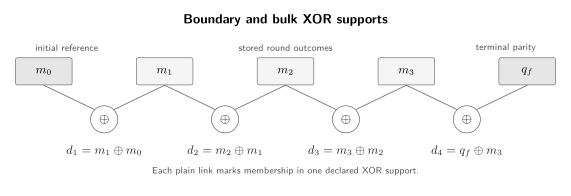
A boundary-closed temporal detector map. The records $m_0$ and $q_f$ require independently justified preparation and compatible destructive-readout references. Links identify the two record bits in each XOR support; they do not denote fault channels, causal independence, or a decoded explanation.

Detector supports form the decoder-facing record

The adjacent-round form is one special case of

$$d_\alpha = \bigoplus_{(j,t)\in R_\alpha}m_{j,t} \oplus c_\alpha,$$

where $R_\alpha$ is a declared support over check labels and times, and $c_\alpha$ contains known sign, frame, or circuit offsets. The defining property is that $d_\alpha$ has a deterministic no-fault value, conventionally zero. A nonzero value establishes that this declared parity relation was violated. It does not establish which physical fault occurred.

Detector class	Parity definition	Required no-fault reference	What a nonzero value establishes
Bulk	$d_t=m_t\oplus m_{t-1}$	unchanged check and stable convention across adjacent rounds	the neighboring outcomes violate their expected equality
Initial boundary	$d_1=m_1\oplus m_0$	preparation fixes the signed reference $m_0$	the first outcome disagrees with the prepared reference
Terminal boundary	$d_f=q_f\oplus m_T$	compatible final readout fixes parity $q_f$ in the same frame	the last check outcome disagrees with terminal parity
General support	$d_\alpha=\bigoplus_{(j,t)\in R_\alpha}m_{j,t}\oplus c_\alpha$	a declared relation deterministic in the no-fault model	support $R_\alpha$ with offset $c_\alpha$ is violated

If any required outcome is missing, invalid, or marked as leakage, every detector that depends on it is unavailable unless the protocol defines another justified gap-spanning deterministic relation. Zero-filling is not neutral: it can suppress a real event or fabricate one. The exported object should therefore include detector validity or erasure information alongside binary values. Decoders owns the subsequent use of this record with priors, correlations, equivalence classes, latency constraints, and recovery or Pauli-frame decisions.

Detector supports describe algebraic parity, not statistical independence. Two detectors may share measurements, a single circuit fault may activate several detectors, and correlated faults may create patterns that imitate separate events. Nor do the edges in a detector diagram assert causal flow from a record bit to a fault. The record remains useful precisely because the circuit declares which relations should vanish; a decoder adds the probabilistic model needed to compare candidate explanations.

Four-Body Z-Check Audit

A finite ledger makes the distinctions concrete. The following experiment is intentionally code independent: it specifies one check and one terminal parity, not a code space or a global decoder. Every conclusion is restricted to the declared circuit, fault list, and record.

Freeze the four-body experiment

Measure

$$g=Z_1Z_2Z_3Z_4$$

for three rounds. Each round uses a fresh $\lvert0\rangle_a$ ancilla and data-control/ancilla-target CNOTs in chronological data order $1,2,3,4$. The sign is $\sigma=0$. Preparation supplies a known $+1$ reference $m_0=0$, and no fault occurs unless a row explicitly inserts one.

After round 3, destructively read the data in Z and define

$$q_f=z_1\oplus z_2\oplus z_3\oplus z_4.$$

The boundary-closed detector record is

$$d_1=m_1\oplus m_0, \qquad d_2=m_2\oplus m_1, \qquad d_3=m_3\oplus m_2, \qquad d_4=q_f\oplus m_3.$$

The terminal parity is compatible with this Z check, but its four fine-grained data bits are not retained in the compact ledger. Their acquisition ends the quantum memory experiment.

Evaluate six declared fault cases

Case	Inserted fault and location	Data Pauli before terminal readout	Stored record m1m2m3	qf	Detector record d1d2d3d4
No fault	no inserted fault	$I$	000	0	0000
$X_2$ before round 1	$X_2$ before the first interaction of round 1	$X_2$	111	1	1000
$X_2$ between rounds 1 and 2	$X_2$ after round 1 and before round 2	$X_2$	011	1	0100
Reported-bit flip in round 2	flip only the reported bit after ideal round-2 readout; latent ideal record 000	$I$	010	0	0110
$X_a$ after the second CNOT of round 2	ancilla X after data 2 and before data 3	$I$	010	0	0110
$Z_a$ after the second CNOT of round 2	ancilla Z after data 2 and before data 3	$Z_3Z_4$	000	0	0000

An $X_2$ present before the first round anticommutes with $g$, so every measured check bit is one and the terminal Z parity is one. Only the initial boundary comparison fires. Inserting the same error between rounds 1 and 2 moves the event to $d_2$. These rows demonstrate onset timing; they do not identify why the $X_2$ occurred.

The reported-bit flip changes only $m_2$, producing neighboring events $d_2=d_3=1$. An $X_a$ after the second CNOT produces exactly the same compact record because it flips the Z-basis ancilla result without propagating to the data. The two mechanisms are physically distinct but locally aliased.

For the $Z_a$ row, only the later CNOTs act after insertion, so forward propagation leaves $Z_3Z_4$ on the data. That operator commutes with this Z check, and terminal Z-basis bits are insensitive to phase flips, hence the all-zero local record. The zero does not certify an error-free state.

Each row admits an independent parity check. For stored record 111 with $m_0=0$ and $q_f=1$, the four XORs are $1,0,0,0$. For 011 with terminal parity 1, they are $0,1,0,0$. For 010 with terminal parity 0, they are $0,1,1,0$. These calculations verify the detector column without using a fault hypothesis. The quantum propagation column is checked separately by commuting only the inserted Pauli through later gates. Keeping those audits separate prevents a desired detector pattern from being used as circular evidence for the assumed data error.

Aliases and silent records limit inference

The map from faults to detector records is not injective: the reported-bit flip and $X_a$ rows both give 0110. A decoder can distinguish mechanisms only through additional checks, correlations, analog information, or a noise prior. Even then it typically infers an equivalence class or a most likely correction, not an observed microscopic cause.

The $Z_a$ row is silent only to this one Z check and its terminal Z parity. Other checks may detect $Z_3Z_4$. Whether that Pauli is a stabilizer, a correctable error, an uncorrectable detectable error, or a logical operator depends on the surrounding code. Calling it harmless, logical, or globally undetectable would all exceed this ledger’s evidence.

There is also a semantic difference between an observed zero and no observation. The $Z_a$ case supplies valid bits whose declared parities evaluate to zero; a lost round instead makes its dependent detectors unavailable. Both situations can leave no activated detector in a naïve binary list, but they imply different likelihoods and different decoder inputs. A mature record carries validity information so that silence caused by a commuting fault is not conflated with silence caused by absent telemetry.

The same caution applies to an unspecified data fault “during round 2.” If an $X_j$ occurs before qubit $j$ interacts, it can change that round’s outcome; after the interaction, its first effect may appear in round 3. An exact fault table must locate the insertion relative to the relevant gate. It must also declare whether faults persist, whether resets work, and which other locations are excluded.

Canonical Owners and Extraction Failure Modes

This page owns the translation from a signed check and an ordered ancilla circuit to raw outcomes, stored syndrome bits, single-fault propagation, and detector supports. It does not absorb its neighboring theories. Pauli Group and Stabilizers owns phase-safe algebraic signatures; Stabilizer Formalism owns projectors, normalizers, logical cosets, and syndrome algebra; and Multi-Qubit Gates owns the general parity instrument and elementary circuit construction. Quantum Instruments owns general CP instruments and disturbance freedom.

The output here is still upstream of inference and code-specific protection. Decoders maps detector records and priors to recovery or frame decisions. Fault-Tolerant Gates owns gadget-containment criteria, flags, verified cats, encoded ancillas, and logical operations. Surface Code owns lattice geometry, the global star-and-plaquette schedule, hook orientation relative to boundaries and logical strings, spacetime decoding graphs, effective distance, and thresholds.

A useful handoff from extraction to decoding contains more than a string of activated locations. It identifies detector supports and offsets, their spacetime coordinates, validity or erasure flags, and the circuit or calibration version that defines the record. The decoder may attach edge probabilities, correlations, or learned likelihoods, but those additions must not rewrite which parity the circuit declared. A handoff to a fault-tolerance proof is different: it supplies the ordered circuit and enumerated quantum-plus-classical consequences for each allowed fault location. That proof then judges the consequences against a code-specific correctable set and acceptance rule.

Do not measure a non-Hermitian group element. A factor $\pm i$ makes a Hermitian Pauli string anti-Hermitian. Convert the algebraic group element to an explicitly signed Hermitian check before assigning binary eigenspaces.

Do not infer the instrument from the observable alone. The projectors fix probabilities, not every conditional disturbance. State that the Lüders instrument is the chosen ideal and distinguish it from apparatus-specific refinements, leakage, or outcome-dependent rotations.

Do not claim logical opacity without a stabilizer premise. A commuting nonstabilizer Pauli may be a logical observable. Fine-grained terminal readout followed by XOR can also expose more information than the coarse check even when its parity is compatible.

Do not merge records with inferences. Raw bit $r$, sign $\sigma$, stored bit $m$, detector $d_\alpha$, and decoded fault hypothesis belong to different layers. Preserve invalid or missing telemetry rather than forcing it into a binary field.

Do not certify fault tolerance from fault-free correctness. A correct ideal projector says nothing about how one ancilla fault spreads. State the allowed fault set and the containment criterion, then test every relevant location. A locally silent record is neither a clean bill of health nor a global logical classification.

A completed extraction audit should therefore answer three questions separately. First, does the no-fault circuit realize the intended signed Lüders branches under the stated preparation and readout conventions? Second, what ordered data error, raw bit, stored bit, and detector pattern results from each declared fault? Third, which conclusions require information outside the local audit, such as other stabilizers, a noise prior, or a gadget-level proof? Keeping the answers separate prevents correctness, diagnosis, and containment from being collapsed into one unsupported claim.

That separation also makes the method portable: a code-family page can replace the geometry, schedule, and containment criterion while preserving the signed-bit and detector-support semantics established here.

Exercises

1. Verify the Projector and Instrument Identities

Let $g=g^\dagger$ and $g^2=I$. For $\Pi_b=[I+(-1)^b g]/2$, prove orthogonality, completeness, and positivity. For a density operator $\rho$, show that $\operatorname{Tr}(\Pi_b\rho\Pi_b)$ is the Born probability and that the unread Lüders map is trace preserving.

Solution

Using $g^2=I$,

$$\Pi_b^2 = \frac{I+2(-1)^b g+g^2}{4} = \Pi_b.$$

Hermiticity of $g$ gives $\Pi_b^\dagger=\Pi_b$, so each idempotent is an orthogonal projector and therefore positive. Direct addition gives $\Pi_0+\Pi_1=I$, while

$$\Pi_0\Pi_1 = \frac{(I+g)(I-g)}{4} = \frac{I-g^2}{4} =0.$$

Cyclicity of trace and idempotence give

$$\operatorname{Tr}(\Pi_b\rho\Pi_b) = \operatorname{Tr}(\rho\Pi_b),$$

the Born probability. Positivity follows because $\Pi_b\rho\Pi_b$ is positive. Finally,

$$\operatorname{Tr}\!\left[\sum_b\Pi_b\rho\Pi_b\right] = \operatorname{Tr}\!\left[\rho\sum_b\Pi_b\right] = \operatorname{Tr}(\rho).$$

Thus each branch is CP and trace-nonincreasing, while their sum is trace preserving.

2. Test Logical Opacity and Its Premise

Let every code state obey $g\lvert\psi_L\rangle=\lvert\psi_L\rangle$. Show that for a fixed Pauli $E$, measuring $g$ on $E\lvert\psi_L\rangle$ reveals only whether $E$ commutes or anticommutes with $g$. Then explain why replacing $g$ by a logical Pauli $\overline Z$ can reveal logical amplitudes.

Solution

If $Eg=s\,gE$ with $s\in\{+1,-1\}$, then

$$gE\lvert\psi_L\rangle = sE g\lvert\psi_L\rangle = sE\lvert\psi_L\rangle.$$

The outcome is fixed by $s$ and is independent of the coefficients of the encoded state. This conclusion uses that $g$ acts as one scalar on the entire code space.

By contrast, suppose $\overline Z\lvert0_L\rangle=\lvert0_L\rangle$ and $\overline Z\lvert1_L\rangle=-\lvert1_L\rangle$. On $\alpha\lvert0_L\rangle+\beta\lvert1_L\rangle$, its measurement has probabilities $|\alpha|^2$ and $|\beta|^2$ and removes coherence between the two logical eigenstates when unread. Although $\overline Z$ commutes with the stabilizer, it is not itself a stabilizer and is not logically opaque.

3. Translate a Signed Check Record

An unsigned circuit measures $P$ and reports $r=0$. Compute the stored bit and signed eigenvalue first for $g=P$, then for the negative check $g=-P$. Repeat for $r=1$, keeping $r$, $\sigma$, and $m$ explicit.

Solution

For $g=P$, $\sigma=0$, so $m=r$. If $r=0$, then $m=0$ and $\lambda_P=\lambda_g=+1$. If $r=1$, then $m=1$ and both eigenvalues are $-1$.

For $g=-P$, $\sigma=1$, so $m=r\oplus1$. At $r=0$, $m=1$: $\lambda_P=+1$ but $\lambda_g=-1$. At $r=1$, $m=0$: $\lambda_P=-1$ but $\lambda_g=+1$. The raw hardware result has not changed; the signed check changes how it must be interpreted and stored.

4. Derive the X-Check Pointer States

Prepare an ancilla in $\lvert+\rangle_a$ and let it control the product $P_X=\prod_{j\in S}X_j$. For a data eigenstate $P_X\lvert\phi_\lambda\rangle=\lambda\lvert\phi_\lambda\rangle$, derive the final ancilla state and explain why the procedure does not perform fine-grained data readout.

Solution

The controlled product maps

$$\lvert+\rangle_a\lvert\phi_\lambda\rangle \longmapsto \frac{\lvert0\rangle_a\lvert\phi_\lambda\rangle +\lvert1\rangle_aP_X\lvert\phi_\lambda\rangle}{\sqrt2} = \frac{\lvert0\rangle_a+\lambda\lvert1\rangle_a}{\sqrt2} \lvert\phi_\lambda\rangle.$$

For $\lambda=+1$ the pointer is $\lvert+\rangle_a$; for $\lambda=-1$ it is $\lvert-\rangle_a$. Every vector within one eigenspace produces the same pointer label. An X-basis ancilla measurement therefore resolves only the product eigenvalue and preserves superpositions within that eigenspace; it never outputs the individual data-qubit X outcomes.

5. Propagate a Mid-Circuit Ancilla Fault

In chronological order $1,2,3,4$, insert $Z_a$ after the second CNOT of a Z-check target-ancilla circuit. Derive the data error. Then perform the dual calculation for $X_a$ at the same location in an X-check control-ancilla circuit, and state what happens to the ancilla readout in each case.

Solution

In the Z-check circuit, the first two CNOTs precede the fault and cannot receive propagated errors from it. At the CNOT involving data 3, target $Z_a$ maps to $Z_3Z_a$; at the next it maps to $Z_4Z_a$. The final operator is therefore

$$Z_3Z_4Z_a.$$

The data error is $Z_3Z_4$. The remaining $Z_a$ commutes with Z-basis readout and does not flip its bit.

In the X-check circuit, the ancilla is the control. Control $X_a$ copies to each later target, producing

$$X_aX_3X_4.$$

The data error is $X_3X_4$. The remaining $X_a$ commutes with X-basis readout and does not flip that bit. The complementary ancilla Paulis, $X_a$ for the Z check and $Z_a$ for the X check, flip their respective readouts without this data fanout.

6. Construct Boundary-Aware Detectors

A check has signed outcomes $m_1,m_2,m_3$. Preparation fixes $m_0=0$, and compatible final readout gives $q_f$. Write the initial, bulk, and terminal detectors. Then generalize to a relation supported on an arbitrary set $R_\alpha$ with a known offset $c_\alpha$. What changes if $m_2$ is invalid?

Solution

The initial detector is $d_1=m_1\oplus m_0=m_1$. The two bulk detectors are

$$d_2=m_2\oplus m_1, \qquad d_3=m_3\oplus m_2,$$

and the terminal detector is $d_4=q_f\oplus m_3$. More generally,

$$d_\alpha = \bigoplus_{(j,t)\in R_\alpha}m_{j,t} \oplus c_\alpha,$$

provided the entire parity is deterministic in the declared no-fault model. If $m_2$ is invalid, both $d_2$ and $d_3$ are unavailable. They may not be computed by replacing $m_2$ with zero. A separately justified relation such as a gap-spanning parity between $m_1$ and $m_3$ could be exported, but only if the protocol explicitly establishes its no-fault determinism.

7. Distinguish Aliased Fault Mechanisms

Use the four-body audit to identify two distinct faults with the same detector record and one nontrivial data fault with a zero detector record. Explain what these facts prove about fault inference and what they do not prove about the code.

Solution

The reported-bit flip in round 2 and $X_a$ after the second CNOT of round 2 both produce stored record 010 and detector record 0110. Therefore the local fault-to-record map is noninjective: observing 0110 cannot uniquely select either mechanism.

The $Z_a$ fault at that location leaves $Z_3Z_4$ on the data but produces detector record 0000. Thus a zero record for this one check and terminal parity does not prove that no data error occurred. Neither fact identifies a logical operator or an uncorrectable error. Additional stabilizers may distinguish the mechanisms or detect $Z_3Z_4$, and the code’s stabilizer and logical cosets decide its eventual classification.

8. Separate Ideal Correctness from Fault Containment

Consider the bare one-ancilla Z-check circuit and the criterion: “every single circuit fault leaves at most one data qubit with an error.” First show that the fault-free circuit measures the intended Z-product. Then test the criterion using a single ancilla fault and state what extra kind of construction would be needed for a containment claim.

Solution

On a computational-basis data string, successive data-control CNOTs place the XOR of the supported bits on the target ancilla. Z-basis ancilla readout therefore distinguishes the $\pm1$ eigenspaces of the Z product, and linearity preserves coherence within each eigenspace. The fault-free circuit realizes the intended ideal parity projectors.

Now insert $Z_a$ after the second CNOT of a weight-four check ordered $1,2,3,4$. Forward propagation produces $Z_3Z_4$ on two data qubits. One fault has therefore left a weight-two data error and violates the stated one-fault/one-data-error criterion, despite ideal correctness.

A valid containment claim needs a code- and fault-model-specific gadget, such as a verified cat ancilla, encoded ancilla, or flag construction, together with a proof that every allowed fault either remains within the correctable set or produces a diagnostic record that the recovery procedure handles. The bare circuit alone supplies neither guarantee.

References

• C. Chamberland and M. E. Beverland, “Flag fault-tolerant error correction with arbitrary distance codes,” Quantum 2, 53, 2018, doi:10.22331/q-2018-02-08-53.
• D. P. DiVincenzo and P. W. Shor, “Fault-tolerant error correction with efficient quantum codes,” Physical Review Letters 77, 3260–3263, 1996, doi:10.1103/PhysRevLett.77.3260.
• C. Gidney, “Stim: a fast stabilizer circuit simulator,” Quantum 5, 497, 2021, doi:10.22331/q-2021-07-06-497.
• Google Quantum AI, “Suppressing quantum errors by scaling a surface code logical qubit,” Nature 614, 676–681, 2023, doi:10.1038/s41586-022-05434-1.
• D. Gottesman, Stabilizer Codes and Quantum Error Correction, Ph.D. thesis, California Institute of Technology, 1997, doi:10.7907/rzr7-dt72.
• P. W. Shor, “Fault-tolerant quantum computation,” in Proceedings of the 37th Annual Symposium on Foundations of Computer Science, 56–65, IEEE Computer Society, 1996, doi:10.1109/SFCS.1996.548464.
• A. M. Steane, “Active stabilization, quantum computation, and quantum state synthesis,” Physical Review Letters 78, 2252–2255, 1997, doi:10.1103/PhysRevLett.78.2252.
• B. M. Terhal, “Quantum error correction for quantum memories,” Reviews of Modern Physics 87, 307–346, 2015, doi:10.1103/RevModPhys.87.307.