Quantum LDPC Codes

Quantum Error Correction and Fault Tolerance places quantum LDPC codes in the active architecture-choice branch of a complete protection claim. Topological Codes owns the common locality, topology, homology, and dimensional-family taxonomy; this page retains sparse-check definitions, rate–distance tradeoffs, the construction landscape, decoding, noisy-check behavior, scheduling, evidence, and overhead without using the 2021 review to claim asymptotically good families exist.

Short Definition

A family of stabilizer codes is quantum low-density parity-check, or qLDPC, when it admits a generating set in which

1. every stabilizer generator acts on at most a constant number of physical qubits; and
2. every physical qubit participates in at most a constant number of those generators,

with both constants independent of the block length.

For a code of length $n$, let $w$ be the largest generator weight and $\Delta$ the largest number of generators incident on one qubit. The LDPC condition is

$$\sup_n w_n<\infty, \qquad \sup_n \Delta_n<\infty.$$

“Low density” describes the sparsity of a parity-check presentation. It does not mean low code rate, small logical distance, weak protection, or geometric locality in a laboratory layout. The surface and toric codes are qLDPC codes because their checks have bounded weight and degree, even though their asymptotic encoding rate vanishes. Conversely, a constant-rate qLDPC code can require long-range physical interactions.

CSS Codes owns the general paired CSS check matrices, nested-code and coset bases, logical quotients, exact axis distances, and split-syndrome algebra. This page is the canonical home for sparse CSS presentations, Tanner graphs, bounded row and column degrees, redundant-check effects, product constructions, asymptotic rate–distance results, qLDPC-specific decoders and schedules, current evidence, and finite-size code assessment. The formulas below remain a compact qLDPC-facing recap of the shared algebra. Decoders owns the common logical-coset objective, algorithm families, noise-model calibration, and real-time contract. Stabilizer Formalism owns the general stabilizer and symplectic algebra. Surface Code owns the geometrically local two-dimensional reference architecture. Fault-Tolerant Gates owns the common gate-gadget criteria and logical-operation mechanisms; this page retains qLDPC-specific connectivity and construction constraints. The Fault-Tolerant Quantum Computing Frontier owns integrated architecture comparisons and dated claims about useful-scale computation. Quantum LDPC and High-Rate Codes owns the qLDPC-specific frontier assessment: finite-size overhead, decoder scaling, hardware embedding, logical operations, and current experiments.

Code Parameters and Asymptotic Language

A binary stabilizer code with parameters $[[n,k,d]]$ embeds $k$ logical qubits in $n$ physical qubits and has distance $d$. It corrects every Pauli error of weight at most

$$t=\left\lfloor\frac{d-1}{2}\right\rfloor$$

under the usual adversarial-distance interpretation.

Three normalized quantities organize qLDPC discussions:

$$R_n=\frac{k_n}{n}, \qquad \delta_n=\frac{d_n}{n}, \qquad \rho_n=\frac{m_n}{n},$$

where $R_n$ is the encoding rate, $\delta_n$ is the relative distance, and $m_n$ is the number of measured checks in the chosen presentation. The number $m_n$ can exceed the stabilizer rank because redundant checks may help detect measurement faults or improve decoding.

Constant rate

A code family has constant rate when there is a fixed $R_0>0$ such that

$$\liminf_{n\to\infty}R_n\geq R_0.$$

This is an asymptotic statement. Calling one finite block “high rate” means only that its ratio $k/n$ is favorable for the comparison being made.

Linear distance

A family has linear distance when there is a fixed $\delta_0>0$ such that

$$\liminf_{n\to\infty}\delta_n\geq\delta_0.$$

Asymptotically good

A code family is asymptotically good when it has both constant rate and linear distance:

$$k_n=\Theta(n), \qquad d_n=\Theta(n).$$

The existence of asymptotically good qLDPC codes was a major open problem for roughly two decades. Lifted-product constructions over non-Abelian groups resolved it in 2022. That theorem is now established. It does not imply that the known asymptotically good families have the best constants, shortest blocks, easiest decoders, most favorable syndrome circuits, or most practical hardware layouts.

The quantum Singleton bound supplies a general ceiling,

$$n-k\geq2(d-1),$$

or asymptotically

$$R+2\delta\leq1.$$

A code can therefore have constant rate and linear distance, but neither can be increased independently without limit.

CSS Parity-Check Description

Most qLDPC constructions used in current theory are Calderbank–Shor–Steane (CSS) stabilizer codes. Let

$$H_X\in\mathbb F_2^{m_X\times n}, \qquad H_Z\in\mathbb F_2^{m_Z\times n}.$$

Each row of $H_X$ is the support vector of an $X$-type stabilizer generator, and each row of $H_Z$ is the support vector of a $Z$-type generator. Commutation requires

$$H_XH_Z^{\mathsf T}=0 \pmod 2.$$

The matrix equation says that every $X$ check and every $Z$ check overlap on an even number of qubits. If $r_X=\operatorname{rank}H_X$ and $r_Z=\operatorname{rank}H_Z$, then

$$k=n-r_X-r_Z.$$

The number of rows can be larger than $r_X+r_Z$. Such dependencies are not automatically waste: redundant syndrome relations can expose measurement errors and support single-shot or data-syndrome decoding in suitable code families.

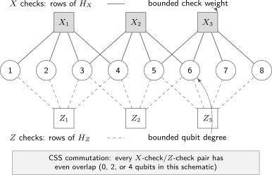
A sparse CSS Tanner graph. Squares are parity checks and circles are physical qubits. Bounded check weight limits the degree of each square; bounded qubit degree limits the degree of each circle. CSS commutation requires every $X$-check/$Z$-check pair to share an even number of qubits.

Syndromes

Represent a $Z$ error by $e_Z\in\mathbb F_2^n$. Its $X$-check syndrome is

$$s_X=H_Xe_Z^{\mathsf T}.$$

Similarly, an $X$ error $e_X$ produces

$$s_Z=H_Ze_X^{\mathsf T}.$$

Under independent $X$ and $Z$ noise, the two binary decoding problems can be treated separately. A depolarizing channel couples them through $Y=iXZ$ events, and exploiting that correlation can materially improve a decoder.

Logical operators and distance

A $Z$-type Pauli commutes with every $X$ check when its support lies in $\ker H_X$. It is a $Z$ stabilizer when its support lies in $\operatorname{row}H_Z$. Therefore

$$d_Z = \min_{\substack{ z\in\ker H_X\\ z\notin\operatorname{row}H_Z }} |z|.$$

Likewise,

$$d_X = \min_{\substack{ x\in\ker H_Z\\ x\notin\operatorname{row}H_X }} |x|, \qquad d=\min(d_X,d_Z).$$

This quotient-space structure is central to quantum decoding. The decoder does not need to identify the physical error exactly. It needs a correction in the same stabilizer coset.

Tanner Graphs

The Tanner graph of a binary parity-check matrix is bipartite:

• one vertex class represents physical qubits or binary variables;
• the other represents parity checks;
• an edge joins check $a$ to qubit $i$ when $H_{ai}=1$.

For a CSS code there are coupled $X$ and $Z$ Tanner graphs sharing the same qubit vertices. The qLDPC constants have direct graph meanings:

$$w =\max_a|\mathcal N(a)|, \qquad \Delta =\max_i|\mathcal N(i)|,$$

where $\mathcal N(v)$ is a vertex neighborhood.

Sparsity matters in three distinct ways.

Syndrome extraction

A check of weight $w$ can be coupled to an ancilla using $w$ data–ancilla interactions rather than an interaction whose support grows with $n$.

Classical inference

Message-passing decoders update local neighborhoods, so one iteration can have work proportional to the number of Tanner edges, which is $O(n)$ for an LDPC family.

Fault containment

A bounded-weight check circuit limits how widely one ancilla fault can spread when the interaction order and verification procedure are designed correctly. Bounded weight alone does not prove fault tolerance: a badly ordered circuit can still create a damaging correlated data error.

How Quantum LDPC Differs from Classical LDPC

The classical analogy is powerful but incomplete.

Classical LDPC	Quantum LDPC
one sparse parity-check matrix $H$	a commuting symplectic matrix, or paired CSS matrices $H_X,H_Z$
decoder seeks a likely error or codeword	decoder seeks a likely logical coset
parity checks may be chosen independently	$X$ and $Z$ checks obey $H_XH_Z^{\mathsf T}=0$
short cycles hinder iterative decoding	orthogonality often forces many even overlaps and short cycles
one observed word supplies the parity violations	syndromes must be measured without reading the logical state
check bits can be assumed reliable in a code-capacity model	repeated quantum operation must tolerate faulty check circuits

Degeneracy

If $S$ is a stabilizer and $E$ is a physical Pauli error, then $E$ and $ES$ have the same logical action on code states and the same syndrome. A maximum-likelihood error decoder chooses one Pauli. A maximum-likelihood coset decoder sums probabilities over all physically different errors with the same logical action:

$$\Pr([E]\mid s) = \sum_{S\in\mathcal S} \Pr(ES\mid s).$$

The most likely individual error need not belong to the most likely coset. This is one reason that directly transplanting a classical decoder can be suboptimal.

The orthogonality bottleneck

Random sparse classical matrices readily give good classical LDPC codes. Two independently chosen sparse matrices almost never satisfy $H_XH_Z^{\mathsf T}=0$. Enforcing commutation while retaining rate, distance, sparsity, and decodability is the structural difficulty that product, homological, expander, and group-based constructions address.

The Hypergraph Product

The hypergraph product converts two classical parity-check matrices into a CSS code. Let

$$H_1\in\mathbb F_2^{r_1\times n_1}, \qquad H_2\in\mathbb F_2^{r_2\times n_2}.$$

Define

$$\begin{aligned} H_X &= \left[ H_1\otimes I_{n_2} \;\middle|\; I_{r_1}\otimes H_2^{\mathsf T} \right],\\ H_Z &= \left[ I_{n_1}\otimes H_2 \;\middle|\; H_1^{\mathsf T}\otimes I_{r_2} \right]. \end{aligned}$$

The code has

$$n=n_1n_2+r_1r_2$$

physical qubits. Commutation follows directly:

$$\begin{aligned} H_XH_Z^{\mathsf T} &= H_1\otimes H_2^{\mathsf T} +H_1\otimes H_2^{\mathsf T}\\ &=0 \pmod 2. \end{aligned}$$

Let

$$k_i=n_i-\operatorname{rank}H_i, \qquad k_i^{\mathsf T} =r_i-\operatorname{rank}H_i.$$

Then the number of logical qubits is

$$k=k_1k_2+k_1^{\mathsf T}k_2^{\mathsf T}.$$

When the classical seed matrices have bounded row and column weights, the product code is qLDPC. Suitable constant-rate classical seeds yield constant-rate quantum codes with distance proportional to $\sqrt n$. This was a decisive construction: it combined bounded checks, positive quantum rate, and growing distance in a general algebraic framework.

The toric code as a product

Take both seed matrices to be the cyclic repetition-code check matrix on $L$ bits. Each is $L\times L$, has rank $L-1$, and has one-dimensional kernel and cokernel. The hypergraph product gives

$$[[2L^2,\,2,\,L]],$$

the toric-code parameter family. Thus the toric code is not conceptually separate from product-code thinking; it is a particularly geometric product of repetition complexes.

Construction Landscape

Product language is useful because a chain complex records qubits, checks, relations among checks, and logical homology in one algebraic object. New constructions change the product or the geometry while preserving $\partial^2=0$, the chain-complex form of stabilizer commutation.

Hyperbolic and homological codes

Topological codes on negatively curved cellulations can achieve constant rate because area grows rapidly with linear size. Their distance is typically smaller than linear, and embedding their interaction graph in ordinary two-dimensional hardware introduces nonlocality. They showed early that vanishing surface-code rate was a consequence of Euclidean geometry rather than of LDPC sparsity itself.

Quantum expander codes

Hypergraph products built from classical expander codes have constant rate, distance of order $\sqrt n$, and efficient small-set-flip decoders with provable guarantees. Expansion ensures that a sufficiently small error has many locally visible syndrome defects. A decoder can then flip a small set whose boundary substantially reduces the syndrome.

The guarantee depends on the expansion and noise assumptions. It should not be transferred automatically to an arbitrary sparse CSS matrix.

Fiber-bundle, balanced-product, and lifted-product codes

Ordinary products repeat local structure in a way that historically limited known qLDPC distance to roughly $\sqrt n$ up to polylogarithmic factors. Twisted products use a group action or bundle structure so that one factor changes while it is transported around another.

The progression was mathematically significant:

• fiber-bundle codes surpassed the $\sqrt n\,\operatorname{polylog}n$ distance barrier;
• lifted-product codes achieved almost-linear distance in a low-rate regime;
• balanced-product codes gave explicit families with improved simultaneous rate and distance exponents;
• lifted products over non-Abelian groups produced constant-rate, linear-distance qLDPC families, resolving the asymptotically good qLDPC conjecture;
• quantum Tanner codes gave a related expander-complex construction with linear distance and efficient decoders under stated local-code conditions.

These are existence and algorithmic results about code families. Their asymptotic proofs may use group sizes, local codes, or expansion constants far from the most useful finite blocks. Practical code discovery remains a finite-length optimization problem.

Quasi-cyclic and bicycle constructions

Quasi-cyclic structure replaces large binary matrices with polynomials or small matrices over a group algebra. It offers:

• compact code specification;
• translation-like symmetries;
• efficient matrix operations;
• structured hardware layouts;
• fewer parameters to search;
• potentially simpler logical-operator bases.

A common bivariate-bicycle CSS form uses two commuting sparse binary matrices $A$ and $B$:

$$H_X=[\,A\mid B\,], \qquad H_Z=[\,B^{\mathsf T}\mid A^{\mathsf T}\,].$$

Because $A$ and $B$ commute,

$$\begin{aligned} H_XH_Z^{\mathsf T} &=AB+BA\\ &=0 \pmod 2. \end{aligned}$$

When $A$ and $B$ are sums of a few monomial shift matrices, checks and qubit degrees remain small. Their two cyclic directions motivate the name bivariate. The algebraic symmetry can also produce a connectivity graph that is the union of a small number of planar layers, although the physical edges need not be short in one plane.

Bivariate-bicycle codes are important finite-size candidates, not a synonym for all qLDPC codes. A 2024 circuit-level study found a family of weight-6 codes with a reported memory threshold near that of the surface code under its stated noise and decoder model. Its representative $[[144,12,12]]$ block used 144 data qubits and 144 measurement ancillas in the proposed syndrome circuit. The comparison projected nearly one million cycles for 12 logical qubits at physical error $10^{-3}$, using 288 physical qubits rather than roughly 3000 in the matched surface-code estimate. Every number in that comparison is model-dependent; the structural achievement is a concrete finite block, circuit, connectivity graph, and decoder that can be audited together.

What the Surface Code Does and Does Not Represent

The toric and surface codes satisfy the qLDPC definition:

$$w=O(1), \qquad \Delta=O(1).$$

For a planar surface-code patch encoding one logical qubit,

$$k=1, \qquad n=\Theta(d^2), \qquad R=\Theta(d^{-2})\to0.$$

The surface code therefore demonstrates that low-density checks can coexist with high circuit-level thresholds and local two-dimensional extraction. It does not demonstrate the constant-rate advantage sought from newer qLDPC families.

The distinction is useful:

Property	Surface-code family	General high-rate qLDPC goal
bounded check weight and degree	yes	yes
Euclidean 2D geometric locality	yes	generally no
asymptotic rate	zero for independent planar patches	bounded away from zero
distance versus block length	$d=\Theta(\sqrt n)$	ideally $d=\Theta(n)$
generic decoder	matching and specialized topological methods	message passing, local search, or construction-specific methods
logical organization	usually one or a few qubits per patch	many coupled logical qubits per block

Neither column dominates without a hardware and workload model. Locality can raise threshold and simplify syndrome extraction. Rate can reduce data-qubit overhead. The relevant comparison includes both.

Decoding Is Coset Inference

The Decoders page derives why a recovery must identify the correct stabilizer coset rather than the microscopic physical error. The qLDPC-specific challenge is to approximate that posterior using a sparse but highly loopy Tanner graph while preserving the $X$–$Z$ correlations and degeneracy imposed by quantum commutation.

Belief propagation

The belief-propagation derivation defines the log-likelihood messages and parity-check update. On a tree they give exact local marginals after enough iterations. qLDPC Tanner graphs contain cycles; in common CSS representations, commutation constraints also create many short loops. Messages then become correlated and BP may oscillate, converge to an inconsistent estimate, or choose a poor representative of a highly degenerate coset.

Useful modifications include damping, randomized schedules, min-sum approximations, correlated $X$–$Z$ messages, guided decimation, and neural message updates. Performance must be reported for the exact code, noise model, number of iterations, stopping rule, and post-processing.

Ordered-statistics post-processing

BP plus ordered-statistics decoding (BP+OSD) uses BP reliabilities to choose a likely information set, solves the syndrome constraint there, and searches nearby low-order alternatives. It is a broadly useful finite-size qLDPC baseline and often rescues BP failures. Its post-processing cost can become a latency bottleneck, so decoder accuracy and tail runtime should be reported together.

Localized and search-based decoders

When a sparse error produces disconnected or weakly connected syndrome clusters, localized-statistics methods solve small regional problems and reconcile them. Beam-search and related methods retain several promising partial corrections instead of committing greedily to one. Both create a tunable accuracy–latency tradeoff.

No benchmark on one code family establishes a universal qLDPC decoder. Structure matters: expansion, quasi-cyclic symmetry, check redundancy, noise bias, erasure information, and circuit-induced correlations can all change the best inference rule.

Provable decoders

Small-set-flip algorithms for quantum expander codes use expansion to prove correction of adversarial errors through weight $\Omega(\sqrt n)$ in early constructions. Later decoders for asymptotically good quantum Tanner and lifted-product codes correct a constant fraction of adversarial errors under their construction hypotheses, with linear or highly parallel runtimes.

Provable correctable weight, stochastic threshold, and finite-size logical error rate are different metrics:

• an adversarial guarantee covers every error below a weight;
• a stochastic threshold describes a distribution as size grows;
• finite-size logical error measures a specified block and operating point.

Faulty Syndrome Measurements

The equations $s=He^{\mathsf T}$ assume perfect check outcomes. Let $\eta_t$ be measurement error in round $t$. A simplified observed syndrome is

$$\widetilde s_t =He_t^{\mathsf T}+\eta_t.$$

With evolving data errors, decoders use differences between rounds and a space–time detector model. A data fault and a measurement fault leave different temporal signatures only when enough syndrome relations and rounds are available.

LDPC does not imply single-shot correction

A single-shot scheme can tolerate noisy syndrome extraction using a bounded number of measurement rounds, typically because redundant local constraints confine syndrome noise or make it itself decodable. Merely having bounded-weight stabilizers does not provide that property. Two qLDPC families can have the same $[[n,k,d]]$, $w$, and $\Delta$ yet very different syndrome redundancy and single-shot behavior.

Circuit distance can be below code distance

An abstract code distance counts data Pauli support. A syndrome circuit adds ancillas, gates, reset, measurement, and time. A set of fewer than $d$ circuit faults may cause a logical failure if one fault propagates to several data qubits or if detector information is missing.

For a concrete implementation, define a detector error model and measure or compute the circuit distance: the minimum number of circuit faults in the model that produces an undetected logical effect. A fault-tolerant extraction schedule aims to preserve the intended effective distance.

From Sparse Checks to a Physical Schedule

Introduce one ancilla for each simultaneously measured check. The data–ancilla interactions form a bipartite graph with maximum degree

$$\chi_{\max}=\max(w,\Delta).$$

If every required edge can be executed directly and each qubit participates in at most one two-qubit gate per layer, König’s line-coloring theorem gives an edge coloring with exactly $\chi_{\max}$ colors. The interaction portion of an idealized extraction round can therefore be scheduled in $\chi_{\max}=O(1)$ layers.

This elegant graph result is not a hardware schedule. It assumes every Tanner edge is physically available and ignores:

• geometric routing or shuttling;
• frequency and laser-addressing conflicts;
• coupler crosstalk;
• ancilla preparation and measurement;
• direction-dependent gates;
• fault-propagation ordering;
• leakage removal;
• unavailable parallelism;
• classical feedforward.

The physical extraction depth can scale even when the abstract code is LDPC.

LDPC locality versus geometric locality

LDPC locality means that each check touches few qubits. Geometric locality means that those qubits are physically near one another. These are different graphs.

For local commuting stabilizer codes in a two-dimensional Euclidean layout, the Bravyi–Poulin–Terhal tradeoff gives

$$kd^2\leq Cn$$

for a constant $C$ fixed by local geometry and on-site dimension. A family with $k=\Theta(n)$ must then have $d=O(1)$. Constant rate and linear distance cannot both be obtained with bounded-range two-dimensional stabilizer checks under those assumptions.

An asymptotically good qLDPC architecture must therefore relax something:

• use long-range couplers;
• move qubits or ancillas;
• embed edges across several layers;
• distribute checks through photonic or modular links;
• simulate nonlocal checks over time;
• use a non-Euclidean or higher-dimensional effective connectivity;
• leave the assumptions of commuting local stabilizer generators.

The cost has not disappeared. It moved from code density into physical connectivity, routing, time, fabrication, or communication.

Logical Operations on a High-Rate Block

Encoding many logical qubits in one block reduces boundary overhead but couples their organization. A logical operator can have support spread across the block, and two logical qubits may not have independent local patches that can simply be moved together.

Candidate mechanisms include:

• transversal Clifford operations supported by product symmetry;
• automorphisms and permutations of a block;
• code switching or teleportation to an auxiliary code;
• generalized lattice surgery and logical Pauli measurements;
• gauge measurements and deformations;
• magic-state injection and consumption.

A memory construction does not automatically provide a universal fault-tolerant instruction set. Logical operations must be assessed for distance preservation, ancilla cost, parallelism, routing, decoder changes, and addressability of individual logical qubits.

Finite-Length Code Assessment

Asymptotic notation suppresses precisely the constants that determine a near-term architecture. A finite qLDPC code card should include:

Item	Required information
algebraic block	$[[n,k,d_X/d_Z]]$, stabilizer ranks, redundant rows, logical-operator basis
sparsity	maximum and distributions of check weight and qubit degree
graph structure	girth, connected components, expansion or quasi-cyclic symmetry, required edge lengths
extraction	ancilla count, interaction depth, gate order, reset, measurement, leakage handling
noise	data, gate, idle, measurement, erasure, leakage, correlation, and range dependence
decoder	algorithm and version, iteration limits, post-processing, training data, latency distribution
performance	logical failure per block and per logical qubit, acceptance, confidence interval, tested rounds
operations	preparation, readout, accessible logical Paulis, Clifford and non-Clifford mechanisms
resources	data, checks, routing, links, buffers, spares, classical compute, and delivered time

Per-block and per-logical-qubit rates

A block encoding $k$ logical qubits can fail on one or several logical coordinates. Let $P_{\mathrm{block}}$ be the probability of any logical failure, and let $p_j$ be the marginal probability that logical qubit $j$ fails. Then

$$\max_jp_j \leq P_{\mathrm{block}} \leq \sum_{j=1}^{k}p_j.$$

Reporting only $P_{\mathrm{block}}$ can make a high-rate code look worse as $k$ grows, while reporting only the average marginal can hide correlated multi-logical failures. Both, together with the logical correlation structure, are useful.

Threshold is not enough

A code–circuit–decoder family has a threshold when increasing size suppresses logical error below a critical physical operating point. The Threshold Theorem owns the general existence, noise-assumption, and overhead statements. Two architectures with similar thresholds can have very different subthreshold prefactors, distances, rates, cycle times, and connectivity costs. For a target block failure $P^\star$, the practical question is

$$\min_{\mathcal C} \left\{ \text{delivered cost}(\mathcal C): P_{\mathrm{block}}(\mathcal C)\leq P^\star \right\},$$

not which crossing occurs at the largest physical-error probability.

Distance verification is itself difficult

Finding the exact distance of a general stabilizer code is computationally hard. Finite-code reports should distinguish:

• a proved distance;
• an exhaustive search result;
• a certified lower bound;
• a heuristic upper bound from a found logical operator;
• a distance inferred from logical-error scaling.

The last is not a substitute for the first four.

Experimental Status

The theory that asymptotically good qLDPC families exist is established. Finite circuit-level qLDPC memories with favorable modeled overhead are established computationally under declared noise and decoder assumptions. Long-range-connected hardware has now executed repeated syndrome circuits for small high-rate blocks. Scalable below-threshold qLDPC error suppression on hardware is not yet established.

In a 2026 superconducting experiment, 32 transmon qubits and overlapping long-range couplers implemented two weight-6 qLDPC codes: a distance-4 bivariate-bicycle code encoding four logical qubits and a punctured distance-3 code encoding six. The reported logical error per logical qubit per cycle was $8.91(17)\%$ and $7.77(12)\%$, respectively. The experiment established simultaneous nonlocal check measurement and repeated qLDPC syndrome operation on the device. Those logical rates did not establish break-even, a threshold, or scalable suppression.

Other processors have implemented nonlocal finite-rate codes, transversal operations, and high-rate logical blocks using transport or reconfigurable arrays. These experiments test connectivity and logical organization. The decisive qLDPC scaling evidence will compare several increasing blocks under comparable circuit noise, decoding, acceptance, and elapsed time.

Common Mistakes

Equating qLDPC with high rate

LDPC constrains check and qubit degree. The surface code is qLDPC and has vanishing rate. Constant rate is an additional property.

Equating bounded check weight with short-range hardware

A weight-6 check can involve six qubits separated across a processor. Weight and geometric diameter are independent.

Calling one finite ratio an asymptotic rate

A $[[144,12,12]]$ code has finite rate $1/12$. It does not by itself define a constant-rate family or prove how $k/n$ behaves as $n\to\infty$.

Using abstract distance as circuit distance

Ancilla faults, hook errors, measurement faults, and time boundaries can lower the minimum number of circuit faults needed for logical failure.

Decoding the error rather than the coset

Physically different errors related by a stabilizer are logically equivalent. The best individual error can lie outside the most probable logical coset.

Reporting a decoder without its stopping and latency rules

BP iteration count, damping, OSD order, search width, timeouts, and failure handling can change both logical error and real-time feasibility.

Assuming qLDPC implies single-shot correction

Single-shot behavior needs syndrome redundancy and confinement or another specific mechanism. It is not part of the LDPC definition.

Comparing only data-qubit counts

High rate can reduce data overhead while increasing measurement ancillas, connectivity layers, routing, cycle time, or classical cost. Compare delivered logical service.

Exercises

Exercise 1: Check CSS commutation

Consider

$$H_X= \begin{pmatrix} 1&1&1&1&0&0\\ 0&0&1&1&1&1 \end{pmatrix}, \qquad H_Z= \begin{pmatrix} 1&1&0&0&1&1\\ 0&0&1&1&1&1 \end{pmatrix}.$$

Does this pair define commuting CSS checks? If so, how many logical qubits does it encode?

Solution

Every row-pair overlap has even size:

$$H_XH_Z^{\mathsf T} = \begin{pmatrix} 0&0\\ 0&0 \end{pmatrix} \pmod 2.$$

Both matrices have rank two. Therefore

$$k=6-2-2=2.$$

The matrices define a $[[6,2,d]]$ CSS code. Determining $d$ requires finding the smallest nontrivial logical representatives; commutation and rank alone do not fix it.

Exercise 2: Distinguish sparse, high-rate, and good

Classify the asymptotic properties of three families:

1. $[[2L^2,2,L]]$;
2. $[[n,n/5,\sqrt n]]$;
3. $[[n,n/5,n/20]]$.

Assume each has bounded check weight and qubit degree.

Solution

All three are qLDPC by assumption.

1. The rate is $1/L^2\to0$ and $d/n\to0$. It is neither constant-rate nor asymptotically good.
2. The rate is $1/5$, but relative distance is $1/\sqrt n\to0$. It is constant-rate but not asymptotically good.
3. The rate is $1/5$ and relative distance is $1/20$. It is asymptotically good.

Exercise 3: Hypergraph-product size

Let $H_1$ be $6\times10$ with rank 6 and $H_2$ be $4\times7$ with rank 4. Compute the hypergraph-product values of $n$ and $k$.

Solution

The physical length is

$$n=(10)(7)+(6)(4)=94.$$

The seed dimensions are

$$k_1=10-6=4, \qquad k_2=7-4=3.$$

Both transpose-code dimensions vanish because each matrix has full row rank:

$$k_1^{\mathsf T}=6-6=0, \qquad k_2^{\mathsf T}=4-4=0.$$

Therefore

$$k=(4)(3)+(0)(0)=12.$$

Exercise 4: Recover the toric-code parameters

Each cyclic repetition seed has shape $L\times L$, rank $L-1$, and distance $L$ for both its kernel and transpose kernel. Use the product formulas to obtain $n$ and $k$.

Solution

The product length is

$$n=L^2+L^2=2L^2.$$

For each seed,

$$k_i=L-(L-1)=1, \qquad k_i^{\mathsf T}=L-(L-1)=1.$$

Thus

$$k=(1)(1)+(1)(1)=2.$$

The seed distances give product distance $L$, yielding $[[2L^2,2,L]]$.

Exercise 5: Schedule an ideal Tanner graph

A qLDPC extraction graph has maximum check weight $w=6$ and maximum qubit degree $\Delta=4$. Every required data–ancilla edge is directly available, and a qubit can participate in only one two-qubit gate per layer. What is the minimum number of interaction layers guaranteed by bipartite edge coloring? Why might hardware need more?

Solution

The maximum graph degree is

$$\chi_{\max}=\max(6,4)=6.$$

König’s line-coloring theorem says a bipartite graph has edge-chromatic number equal to its maximum degree, so six interaction layers suffice and are necessary in the worst case.

Hardware may need extra layers for routing, unavailable long-range edges, crosstalk restrictions, gate direction, ancilla preparation and measurement, leakage handling, or a fault-propagation order that differs from an arbitrary edge coloring.

Exercise 6: Identify a degenerate correction

Errors $E_1$ and $E_2$ have the same syndrome and satisfy $E_2=E_1S$ for stabilizer $S$. A decoder observes that $\Pr(E_1\mid s)=0.15$ and $\Pr(E_2\mid s)=0.12$. A different logical coset contains one candidate with probability $0.20$. Can the decoder choose the most likely individual error and be maximum-likelihood at the logical level?

Solution

No. The first logical coset already has probability at least

$$0.15+0.12=0.27,$$

which exceeds $0.20$. Choosing the most likely individual candidate would select the wrong logical coset in this partial example. Logical maximum-likelihood decoding sums probabilities over stabilizer-equivalent errors.

Exercise 7: Apply the 2D locality tradeoff

Suppose a geometrically local two-dimensional commuting stabilizer family has $k=Rn$ for constant $R>0$. Use $kd^2\leq Cn$ to bound $d$.

Solution

Substitution gives

$$(Rn)d^2\leq Cn,$$

so

$$d^2\leq\frac{C}{R}, \qquad d=O(1).$$

Thus a constant-rate family cannot also have growing distance under the stated two-dimensional bounded-range commuting-stabilizer assumptions. A high-rate, growing-distance architecture must relax at least one assumption.

Exercise 8: Classify an experimental result

A device executes all checks of a $[[32,6,3]]$ qLDPC code for 20 rounds and reports a 7% logical error per logical qubit per cycle. What has been established, and what additional evidence is needed for below-threshold scaling?

Solution

The experiment establishes encoding and repeated syndrome extraction for a finite high-rate sparse code on that device, together with a measured logical metric under its decoder and operating conditions.

Below-threshold scaling needs comparable experiments on a code family with increasing protection, showing logical failure decreases as distance grows. The noise model, circuit schedule, decoder, number of rounds, acceptance, elapsed time, and confidence analysis must remain comparable. One finite block and one logical rate cannot establish a threshold.

References

1. R. G. Gallager, Low-Density Parity-Check Codes (MIT Press, 1963).
2. A. R. Calderbank and P. W. Shor, “Good quantum error-correcting codes exist,” Physical Review A 54, 1098–1105 (1996). doi:10.1103/PhysRevA.54.1098
3. A. M. Steane, “Multiple-particle interference and quantum error correction,” Proceedings of the Royal Society A 452, 2551–2577 (1996). doi:10.1098/rspa.1996.0136
4. D. J. C. MacKay, G. Mitchison, and P. L. McFadden, “Sparse-graph codes for quantum error correction,” IEEE Transactions on Information Theory 50, 2315–2330 (2004). doi:10.1109/TIT.2004.834737
5. N. P. Breuckmann and J. N. Eberhardt, “Quantum low-density parity-check codes,” PRX Quantum 2, 040101 (2021). doi:10.1103/PRXQuantum.2.040101
6. J.-P. Tillich and G. Zémor, “Quantum LDPC codes with positive rate and minimum distance proportional to the square root of the blocklength,” IEEE Transactions on Information Theory 60, 1193–1202 (2014). doi:10.1109/TIT.2013.2292061
7. A. Leverrier, J.-P. Tillich, and G. Zémor, “Quantum expander codes,” in 2015 IEEE 56th Annual Symposium on Foundations of Computer Science, 810–824 (2015). doi:10.1109/FOCS.2015.55
8. M. B. Hastings, J. Haah, and R. O’Donnell, “Fiber bundle codes: breaking the $n^{1/2}\operatorname{polylog}(n)$ barrier for quantum LDPC codes,” in Proceedings of STOC 2021, 1276–1288 (2021). doi:10.1145/3406325.3451005
9. P. Panteleev and G. Kalachev, “Quantum LDPC codes with almost linear minimum distance,” IEEE Transactions on Information Theory 68, 213–229 (2022). doi:10.1109/TIT.2021.3119384
10. N. P. Breuckmann and J. N. Eberhardt, “Balanced product quantum codes,” IEEE Transactions on Information Theory 67, 6653–6674 (2021). doi:10.1109/TIT.2021.3097347
11. P. Panteleev and G. Kalachev, “Asymptotically good quantum and locally testable classical LDPC codes,” in Proceedings of STOC 2022, 375–388 (2022). doi:10.1145/3519935.3520017
12. A. Leverrier and G. Zémor, “Quantum Tanner codes,” in 2022 IEEE 63rd Annual Symposium on Foundations of Computer Science, 872–883 (2022). doi:10.1109/FOCS54457.2022.00117
13. S. Bravyi, D. Poulin, and B. M. Terhal, “Tradeoffs for reliable quantum information storage in 2D systems,” Physical Review Letters 104, 050503 (2010). doi:10.1103/PhysRevLett.104.050503
14. N. Baspin and A. Krishna, “Quantifying nonlocality: how outperforming local quantum codes is expensive,” Physical Review Letters 129, 050505 (2022). doi:10.1103/PhysRevLett.129.050505
15. J. Roffe, D. R. White, S. Burton, and E. T. Campbell, “Decoding across the quantum low-density parity-check code landscape,” Physical Review Research 2, 043423 (2020). doi:10.1103/PhysRevResearch.2.043423
16. S. Bravyi et al., “High-threshold and low-overhead fault-tolerant quantum memory,” Nature 627, 778–782 (2024). doi:10.1038/s41586-024-07107-7
17. M. A. Tremblay, N. Delfosse, and M. E. Beverland, “Constant-overhead quantum error correction with thin planar connectivity,” Physical Review Letters 129, 050504 (2022). doi:10.1103/PhysRevLett.129.050504
18. Q. Xu et al., “Constant-overhead fault-tolerant quantum computation with reconfigurable atom arrays,” Nature Physics 20, 1084–1090 (2024). doi:10.1038/s41567-024-02479-z
19. Y. Hong, E. Durso-Sabina, D. Hayes, and A. Lucas, “Entangling four logical qubits beyond break-even in a nonlocal code,” Physical Review Letters 133, 180601 (2024). doi:10.1103/PhysRevLett.133.180601
20. L. Pecorari, S. Jandura, G. K. Brennen, and G. Pupillo, “High-rate quantum LDPC codes for long-range-connected neutral atom registers,” Nature Communications 16, 1111 (2025). doi:10.1038/s41467-025-56255-5
21. N. Berthusen et al., “Toward a 2D local implementation of quantum low-density parity-check codes,” PRX Quantum 6, 010306 (2025). doi:10.1103/PRXQuantum.6.010306
22. T. Hillmann et al., “Localized statistics decoding for quantum low-density parity-check codes,” Nature Communications 16, 8214 (2025). doi:10.1038/s41467-025-63214-7
23. K. Wang et al., “Demonstration of low-overhead quantum error correction codes,” Nature Physics 22, 308–314 (2026). doi:10.1038/s41567-025-03157-4
24. M. Ye, D. Wecker, and N. Delfosse, “Beam search decoder for quantum low-density parity-check codes,” PRX Quantum 7, 033002 (2026). doi:10.1103/6k5x-ztqt

Further Connections

• Why Quantum Error Correction Is Possible supplies the Knill–Laflamme condition and explains why syndrome measurements preserve logical amplitudes.
• Surface Code develops the most mature geometrically local qLDPC family and its circuit-level benchmark conventions.
• Color Codes owns the local 2-colex family and its gate and decoder tradeoffs; this page retains sparsity, Tanner graphs, product constructions, rate–distance asymptotics, schedules, and evidence.
• Common Noise Models distinguishes the independent, biased, erasure, leakage, correlated, and nonstationary models that change decoder performance.
• Resource Estimation shows how finite rate, check connectivity, logical operations, decoding, and hardware assumptions replace a surface-code patch multiplier in a physical resource ledger.
• Resource Estimation Tools provides the reproducible software workflow for evaluating those models.
• Modular Architectures provides one route to realizing sparse but nonlocal Tanner edges through links and distributed modules.
• Reporting Standards gives the provenance, uncertainty, postselection, code, and data record needed for a finite-code comparison.
• Quantum Information Roadmap places qLDPC codes after channels, stabilizers, syndromes, and baseline code families.