Modular Architectures

A modular quantum architecture composes a larger processor, simulator, sensor, or networked instrument from smaller quantum systems whose boundaries and interfaces are explicit. Local operations occur inside modules. Declared services cross module boundaries: coherent state transfer, heralded entanglement, remote gates, transported matter, joint measurement, or measurement-mediated fusion. A classical control plane schedules those services, tracks their state, and closes feedback loops.

Modularity is therefore not synonymous with optical networking, separate cryostats, chiplets, or distributed algorithms. A segmented ion trap can have modules connected by ion transport. Separate superconducting dies can be modules connected by microwave couplers. A photonic machine can distribute state generation, switching, delay, detection, and decoding among rack-mounted modules. Two distant matter registers can use photons only to prepare Bell pairs. What makes each system modular is the architectural contract at its boundaries.

The decisive question is not whether two modules can become entangled once. It is:

Can the complete machine supply boundary-crossing operations with the rate, quality, timing, observability, fault containment, and sustained availability required by its workload and error-correction protocol?

Purpose and Canonical Scope

This page is the canonical home for composing quantum modules into one physical machine. It owns:

• module boundaries, roles, interfaces, capability descriptors, and service semantics;
• quantum, control, timing, calibration, and maintenance planes;
• graph topology, cut capacity, contention, routing, and resource inventory;
• deterministic and heralded fabrics as architecture choices;
• entanglement buffering, memory age, queue stability, and scheduling;
• local versus intermodule error correction and decoder-visible link faults;
• failure domains, redundancy, replaceability, availability, and common-mode risk;
• platform-neutral evidence standards for modular processors.

Interconnects and Transduction owns the accepted-input-to-usable-output physics of a link: conversion, transmission, capture, mode matching, efficiency, added noise, bandwidth, and accepted rate. Quantum Teleportation owns the protocol derivation and no-signalling identity. Quantum Memories owns the write–store–read channel. This page uses those services as architectural primitives and asks how many are needed, when they are available, how they are scheduled, and what happens when they fail.

Quantum Repeaters owns long-distance chain mechanics. Quantum Network Architectures owns end-user, multiuser, and multidomain network organization. Distributed Quantum Computing owns workload partitioning, teledata, telegates, distributed compilation, and program-level execution semantics. Network verification has its own network-facing canonical home. The present boundary is the integrated machine, including physically separated modules when they are operated as one processor.

The Architecture Contract

A modular design is more than a graph of boxes. It is a closed contract among the workload, module capabilities, boundary services, classical control, error correction, and evidence.

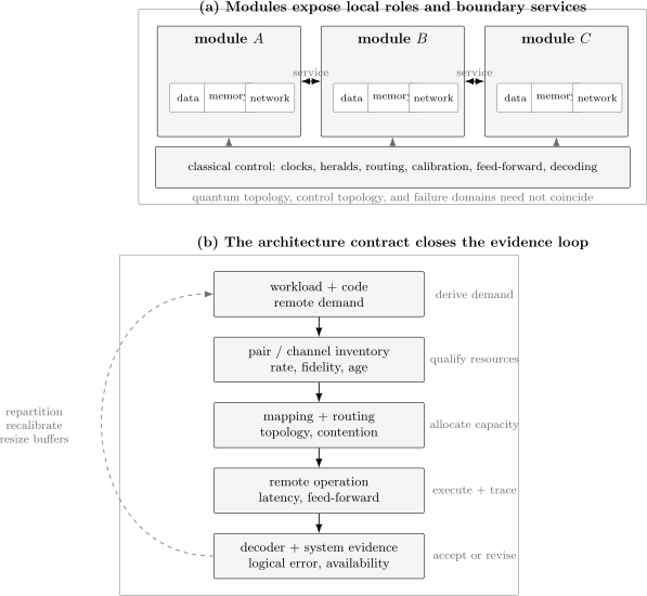
A modular machine has at least two coupled planes. The quantum plane contains local data, memory, ancilla, and network roles plus boundary services. The classical plane carries clocks, heralds, routing decisions, calibration state, feed-forward, and decoder information. A complete contract then maps workload demand into resource inventory, scheduling, execution, and system evidence. Evidence feeds back into partitioning, buffer sizes, calibration, and acceptance limits.

One compact representation is

$$\mathcal A = \left( G,\, \{\mathcal M_i\},\, \{\mathcal S_e\},\, \mathcal C,\, \mathcal F,\, \mathcal E \right),$$

where:

• $G=(V,E)$ is the physical service graph;
• $\mathcal M_i$ is the capability contract of module $i$;
• $\mathcal S_e$ is the service contract on boundary $e$;
• $\mathcal C$ is the control, timing, and scheduling system;
• $\mathcal F$ is the fault-management and error-correction design;
• $\mathcal E$ is the evidence and acceptance specification.

Removing any term creates an incomplete architecture claim. A high-fidelity edge without a scheduler may not deliver useful operations. A scheduler without calibrated edge state may route through stale resources. A fault model without physical failure domains may assume independence where a shared switch, pump, controller, cable, vacuum system, or refrigerator creates correlation.

What Counts as a Module?

A module is an ownership boundary for state and services, not a universal physical size. The same machine may have a hierarchy:

1. A local gate zone or code patch.
2. A chiplet, die, trap segment, cavity register, or photonic subsystem.
3. A packaged processor with local control and readout.
4. A cryostat, vacuum chamber, optical table, or rack.
5. A geographically separated node.

Calling every item a module without naming the level hides the relevant boundary. A transported ion crossing two gate zones and a telecom photon crossing $35\,\mathrm{km}$ both cross interfaces, but they have different loss, latency, clock, maintenance, and fault-domain contracts.

For a declared level, module $i$ should expose a capability record such as

$$\mathcal M_i = \left( Q_i,\, A_i,\, N_i,\, L_i,\, R_i,\, K_i,\, \Theta_i \right).$$

Here $Q_i$ denotes data capacity, $A_i$ local ancillas and memories, $N_i$ network ports, $L_i$ native local operations, $R_i$ readout and reset capabilities, $K_i$ concurrency constraints, and $\Theta_i$ the calibrated operating region. A count of physical qubits is only one component.

Data, memory, and network roles

Architectures often assign different physical qubits or modes to different roles:

• data stores computational or sensing state;
• memory protects state while a probabilistic service is attempted;
• network couples to a flying carrier or boundary bus;
• ancilla supports local gates, purification, syndrome extraction, or teleportation;
• buffer holds accepted but not yet consumed entanglement.

One device can time-share roles, but role changes consume operations and can couple error channels. A communication spin repeatedly optically excited next to a nuclear memory is not equivalent to two independent resources. A superconducting transmon used to emit and capture photons may be unavailable for local gates. A photonic delay line is a memory with fixed routing and loss, not a free queue.

A module must be closed locally

A useful module can initialize, manipulate, measure, and recover enough local state to honor its contract. A chip containing good qubits but depending on an undeclared external controller, clock, detector, or cooling resource is a component, not yet a closed module at that boundary. Conversely, a module need not be computationally universal if its role is specialized. It may be an entanglement factory, memory bank, decoder-adjacent syndrome engine, magic-state factory, router, or sensor head.

Why Modularize?

Modularity trades one scaling problem for a structured set of local and boundary problems. It can be compelling, but it is never free.

Yield and bounded complexity

Smaller repeated units may be easier to fabricate, screen, package, calibrate, and replace than one all-required assembly. If a monolithic device accepts only when all $N$ independent components pass with probability $y$, its idealized yield is

$$Y_{\mathrm{all}} = y^N.$$

Modules can be screened before assembly, and a system can include spares or route around failures. The benefit depends on the real graph constraint, correlations, connector yield, test coverage, and replacement cost. Materials and Fabrication Interface owns that full yield analysis.

Locality and control fan-out

Spectral crowding, wiring, optical access, cross-talk, calibration graphs, and real-time control can become harder as one local register grows. Repeating bounded modules can cap some local coordination costs and support hierarchical calibration. It can also replicate expensive control hardware and introduce new synchronization problems.

Specialization

Different modules can optimize conflicting tasks. A long-lived memory need not be the fastest network emitter. A processor need not place every lossy switch next to every data qubit. A heterogeneous design can separate computation, storage, communication, readout, and resource-state production.

Specialization is useful only if conversion and movement costs fit the workload. A superior memory with a poor write–read interface may lower end-to-end performance.

Fault containment and serviceability

A module boundary can limit the effect of a bad calibration, leakage event, failed component, thermal excursion, or maintenance operation. Replaceable units can improve repair time. These are architectural possibilities, not automatic properties. Shared infrastructure can turn nominally separate modules into one common failure domain.

The boundary tax

Crossing a boundary generally costs more than a local operation. A useful first-order decomposition is

$$\begin{aligned} T_{\mathrm{job}} &= T_{\mathrm{local}} + T_{\mathrm{boundary}} \\ &\quad+ T_{\mathrm{wait}} + T_{\mathrm{classical}}, \\ P_{\mathrm{fail}} &\lesssim P_{\mathrm{local}} + P_{\mathrm{boundary}} \\ &\quad+ P_{\mathrm{memory}} + P_{\mathrm{control}}. \end{aligned}$$

The second line is a small-error bookkeeping approximation, not an exact identity. Boundary count alone is insufficient because errors may be coherent, correlated, heralded, or decoder-visible.

Modularity wins only when bounded local complexity, yield, specialization, maintenance, or connectivity outweigh this boundary tax for a declared task.

Boundary Services

An edge in an architecture graph must say what it provides. The following services are operationally distinct.

Deterministic coherent transfer

A state is emitted from one module, propagated, and captured by another. The desired map is approximately

$$\rho_A \longmapsto \rho_B,$$

with a channel contract for arbitrary accepted inputs. Loss during transfer can irreversibly remove unknown data unless the encoding detects or corrects it. Microwave cables, resonator buses, flying photons, and shuttled matter can all implement versions of this service.

Heralded entanglement

Repeated attempts prepare a state such as

$$\lvert\Phi^+\rangle_{AB} = \frac{ \lvert00\rangle+\lvert11\rangle }{\sqrt2},$$

and a classical event declares whether the resource was accepted. Failed attempts ideally leave protected data intact. The service contract includes conditional state quality, false herald probability, attempt rate, memory disturbance, reset, and accepted throughput.

Entanglement-assisted remote operation

An accepted Bell pair, local operations, measurements, classical messages, and feed-forward implement a remote gate or state transfer. The quantum channel can be used before data enters the protocol, allowing loss to be handled by repetition at the resource-generation stage. The resulting operation is deterministic only conditioned on a usable resource already being available and completion of the classical feed-forward.

Transported matter

Ions, atoms, electrons, or other carriers move between zones. Transport can preserve state and convert a sparse interaction graph into a reconfigurable one. Its ledger includes motional excitation, loss, junction contention, cooling, waveform calibration, and the time during which destination zones are occupied.

Joint measurement and fusion

Some architectures never transfer a persistent data state across the boundary. They interfere carriers, perform a parity measurement, or fuse resource states. The output may be a classical result, an edge in a graph state, or a syndrome relation. Success probability, erasure flags, detector dead time, feed-forward, and graph-state percolation then matter more than a conventional two-qubit gate fidelity.

These services should not be collapsed into a single number called connectivity. Interconnects and Transduction develops their physical channel contracts.

Topology, Demand, and Cut Capacity

Let $G=(V,E)$ be the service graph. Edge $e$ has usable capacity $c_e$, measured in accepted Bell pairs, transfers, fusions, or remote operations per second under a declared quality threshold. Let $D_{ij}$ be the workload demand from module $i$ to module $j$ in the same units.

For a cut $S\subset V$, define

$$\begin{aligned} C(S) &= \sum_{e\in\delta(S)} c_e, \\ D(S) &= \sum_{\substack{i\in S\\j\notin S}} \left(D_{ij}+D_{ji}\right), \end{aligned}$$

where $\delta(S)$ is the set of edges crossing the cut. A necessary stability condition is

$$D(S)<C(S) \qquad \text{for every sustained cut}.$$

If a workload requires $B(S)$ boundary resources across the cut, its idealized communication time obeys

$$T_{\mathrm{boundary}} \ge \max_{S\subset V} \frac{B(S)}{C(S)}.$$

This bound ignores contention inside modules, startup latency, quality classes, and stochastic supply, so it is optimistic. It is nevertheless useful: no compiler can route around a genuine capacity bottleneck without changing the workload partition, service graph, or resource protocol.

Degree is not capacity

A complete graph with weak, serially shared edges can have less usable capacity than a sparse graph with parallel high-rate links. Likewise, all-to-all reachability does not imply all-to-all simultaneity. A central optical switch, common resonator, shared transport junction, or single network qubit may serialize nominally independent edges.

Dynamic topology

Optical switching, atom rearrangement, ion transport, tunable couplers, and software-defined routing can change $G(t)$. Reconfiguration takes time and can invalidate calibrations. A dynamic graph therefore needs both a connection schedule and a transition contract:

$$G_k \xrightarrow[\tau_{\mathrm{reconf}}]{\text{validated transition}} G_{k+1}.$$

The useful topology is the graph that can be reached, calibrated, and held while the workload runs.

Stochastic Supply and Entanglement Inventory

Heralded resources are produced randomly. If one attempt succeeds with probability $p$ and $M$ statistically independent modes are attempted in parallel, the probability of at least one success is

$$p_{\mathrm{eff}} = 1-(1-p)^M.$$

With attempt period $\tau$, the optimistic raw rate is

$$R_{\mathrm{raw}} = \frac{p_{\mathrm{eff}}}{\tau}.$$

If reset, switching, qualification, purification, and memory acceptance retain a fraction $q$, then

$$R_{\mathrm{use}} = qR_{\mathrm{raw}}.$$

The independence assumption can fail through shared emitters, detector dead time, switch contention, pump limits, or correlated drift. Multiplexing gains must be measured at the accepted output, not inferred from mode count.

Inventory has age and quality

A Bell pair is not a fungible timeless token. Record at least

$$b_k = \left( i_k,\, j_k,\, t_k,\, F_k,\, \chi_k,\, \nu_k \right),$$

where $(i_k,j_k)$ are endpoints, $t_k$ is creation time, $F_k$ a qualified quality estimate, $\chi_k$ the calibration or phase-frame context, and $\nu_k$ the protocol version. A scheduler that knows only the inventory count can consume an expired pair or combine resources produced under incompatible settings.

If stored coherence decays approximately as $\exp(-t/T_{\mathrm{mem}})$, a pair waiting for time $t_w$ carries a memory factor

$$\eta_{\mathrm{mem}}(t_w) = \exp\!\left( -\frac{t_w}{T_{\mathrm{mem}}} \right).$$

The exact channel may be dephasing, relaxation, leakage, or non-Markovian; the exponential is an illustrative service model.

Queue stability

Let $\lambda$ be sustained demand and $\mu$ sustained usable supply for one resource class. A necessary queue-stability condition is

$$\lambda<\mu.$$

Running near $\lambda/\mu=1$ can still produce long delays and expired resources. Under the idealized $M/M/1$ model,

$$W = \frac{1}{\mu-\lambda},$$

where $W$ is mean time in the system. Real entanglement factories are often bursty, multi-class, finite-buffer queues with setup times, so measured tail latency and expiry probability are more informative than this mean.

Produce on demand or ahead of demand?

On-demand generation reduces idle decoherence but places stochastic latency on the critical path. Pre-generation hides latency but requires memories, inventory tracking, and expiry policy. A hybrid policy maintains a target stock and regenerates after consumption. The best policy depends on workload burstiness, memory lifetime, pair generation rate, and the cost of disturbing data while attempts run.

Mapping, Routing, and Scheduling

The compiler sees a logical interaction graph $H=(Q,E_H)$ and must map it onto modules and boundary services. For a static partition $\pi:Q\to V$, a simple cut objective is

$$\mathcal C_{\mathrm{cut}}(\pi) = \sum_{(a,b)\in E_H} w_{ab}\, \mathbf 1\!\left[ \pi(a)\ne\pi(b) \right],$$

where $w_{ab}$ weights repeated or expensive interactions. Minimizing this quantity is useful but incomplete. It ignores edge rate, pair age, local capacity, concurrent gates, measurement timing, and error-correction layout.

A practical scheduler must coordinate:

• local gates and measurements;
• link attempts and reset;
• memory occupancy and pair expiry;
• switch, bus, or junction contention;
• classical herald and feed-forward latency;
• decoder deadlines;
• calibration windows and unavailable resources;
• retries, rerouting, and abort semantics.

Move data or move entanglement?

Direct state transfer moves the data itself. Teleportation moves an entanglement resource and later consumes it with local operations. Transported matter changes the physical location of the carrier. Circuit rewriting can instead move the operation, for example by placing a resource-state factory near its consumers.

The choice should minimize an end-to-end cost such as

$$\begin{aligned} \mathcal J ={}& \alpha T + \beta P_{\mathrm{logical}} + \gamma N_{\mathrm{pair}} \\ &+ \delta Q_{\mathrm{memory}} + \epsilon E_{\mathrm{classical}}. \end{aligned}$$

with weights set by the task. No universal routing strategy minimizes all terms.

Burstiness matters

A circuit can have modest average remote-gate count but intense bursts at code deformation, lattice surgery, fan-out, or resource injection. Provisioning only for the average creates stalls. Architecture studies should report remote-demand traces or at least peak-to-mean ratios and cut-specific bursts.

Remote Operations and Their Error Ledger

Suppose a remote operation consumes one qualified Bell pair. To first order in small stochastic error probabilities,

$$\begin{aligned} p_{\mathrm{remote}} \lesssim{}& p_{\mathrm{pair}} + p_{\mathrm{local},A} + p_{\mathrm{local},B} \\ &+ p_{\mathrm{meas}} + p_{\mathrm{feed}} + p_{\mathrm{wait}}. \end{aligned}$$

This ledger is deliberately architectural. The terms must be replaced by a channel model when coherent errors, leakage, correlated phase noise, false heralds, or bias matter. A conditional Bell-state fidelity does not include the rate at which such pairs arrive or the decoherence inflicted on data during rejected attempts.

The corresponding latency can be decomposed as

$$\begin{aligned} T_{\mathrm{remote}} ={}& T_{\mathrm{resource}} + T_{\mathrm{local}} + T_{\mathrm{measure}} \\ &+ T_{\mathrm{message}} + T_{\mathrm{feedforward}}. \end{aligned}$$

Pauli-frame updates can defer some physical corrections, but they do not remove message delivery, frame consistency, or downstream scheduling dependencies. The Quantum Teleportation page gives the protocol identity; this page keeps the machine-level ledger.

Local and Intermodule Error Correction

Modularity can be placed at several levels of an error-corrected architecture:

1. Physical modules provide qubits used by one code block spanning boundaries.
2. Each module hosts a code patch, and boundaries implement joint logical measurements.
3. Each module hosts complete logical qubits, and purified or encoded Bell pairs mediate logical gates.
4. Specialized modules produce encoded resources consumed elsewhere.

These choices change the required link fidelity, rate, memory, and decoder.

Network noise need not equal local noise

Heralding, purification, error detection, and repeated syndrome extraction can tolerate a boundary channel that is noisier than local gates. Nickerson, Li, and Benjamin showed in architecture-specific simulations that very noisy photonic links can coexist with substantially lower local error rates. Their thresholds are not universal constants. They depend on the cell size, noise model, protocol, timing, and decoder.

Recent simulations continue to show that code family and distributed primitive matter. A transversal nonlocal operation, lattice-surgery measurement, and logical teleportation can consume different numbers of Bell pairs and expose different correlated faults. A claim that a code is fault-tolerant locally does not establish fault tolerance across a link.

Erasures and flags are valuable

Known loss can be easier for a decoder than an unflagged Pauli error. A link contract should propagate:

• failure or success heralds;
• confidence or soft information when calibrated;
• pair age and endpoint identity;
• leakage and reset outcomes;
• correlated-event identifiers;
• calibration version and time.

Discarding these labels and replacing the link by an average depolarizing probability can lose useful structure or hide dangerous correlations.

Distributed syndrome timing

If a stabilizer spans modules, its syndrome cycle may wait for a stochastic resource. The decoder then receives an irregular space–time graph rather than a synchronous rectangular lattice. Timeouts, missing checks, delayed checks, and repeated attempts need explicit representation. A cycle-time average is not enough; long tails can dominate memory error.

Logical evidence must scale

A small code can detect errors without demonstrating suppression. The relevant test compares increasing code size or protection level under the same architecture, including link attempts, waiting, decoding, and classical latency. Surface Code owns the code itself; modular studies must state how its checks are physically distributed.

The Classical Control Plane

The quantum graph is only half the machine. A modular architecture needs a classical control plane whose state transitions are at least as explicit as the quantum protocol.

Required records

For each attempt or resource, record:

• globally unique operation and module identifiers;
• source and destination ports;
• trigger and detection timestamps;
• herald pattern and qualification result;
• calibration and firmware versions;
• phase or Pauli-frame context;
• memory location and expiry time;
• retry, timeout, reroute, and abort reason;
• downstream consumer and decoder association.

Without traceability, a measured end-to-end fidelity cannot be attributed to the resources that produced it.

Clock and phase

Frequency and phase errors accumulate across modules. A simple relative phase model is

$$\begin{aligned} \phi_{AB}(t) ={}& \phi_{AB}(0) \\ &+ \int_0^t \left[ \omega_A(t')-\omega_B(t') \right]dt' \\ &+ \phi_{\mathrm{path}}(t). \end{aligned}$$

The path term can include fibre motion, cable delay, optical phase, converter pump phase, or switch state. Some two-photon protocols reject common optical phase; others require active stabilization. Time-bin, polarization, frequency, and microwave encodings move the burden rather than eliminate it.

Feed-forward deadlines

Let $T_d$ be the time available before stored data or the code schedule becomes invalid. The complete loop must satisfy

$$\begin{aligned} T_{\mathrm{detect}} &+ T_{\mathrm{classify}} \\ &+ T_{\mathrm{route}} + T_{\mathrm{message}} \\ &+ T_{\mathrm{actuate}} < T_d. \end{aligned}$$

Benchmarks that time only the classifier omit acquisition, transport, queueing, and actuator latency. Control, Readout, and Calibration owns the full local loop; modularity adds cross-module state consistency.

Control topology and quantum topology differ

Two quantum modules may share one clock, FPGA, switch, laser, detector bank, or decoder. Conversely, one physical module may contain several independent controllers. Architecture diagrams should show both topologies, because a shared classical component can serialize operations or create a common-mode failure.

Failure Domains, Availability, and Replacement

A module boundary is valuable only if failures respect it often enough to aid containment and repair.

Map physical fault domains

Examples include:

• a chip, package, connector, cable, or fibre;
• one laser, microwave source, pump, switch, or detector bank;
• a vacuum chamber or cryogenic stage;
• a clock, controller, network switch, or decoder process;
• one calibration model or software release;
• a shared power, cooling, magnetic, or vibration environment.

A single event can cross many logical module boundaries. The fault model should identify both local and common causes.

Series availability

If all $n$ independent modules must be available and module $i$ has availability $A_i$, the idealized system availability is

$$A_{\mathrm{series}} = \prod_{i=1}^{n} A_i.$$

For $n$ identical modules with $A_i=0.999$, one thousand all-required modules have only

$$A_{\mathrm{series}} = 0.999^{1000} \approx 0.368.$$

Real modular systems use spares, degraded modes, rerouting, and repair. They also have correlated failures, so neither the independent series model nor a component uptime alone predicts service availability.

Replaceability is a verified property

An interchangeable module must satisfy more than mechanical fit. Replacement requires:

• compatible physical, optical, electrical, thermal, and vacuum interfaces;
• a machine-readable capability and calibration descriptor;
• bounded parameter variation;
• automated qualification;
• preserved logical identity or a migration protocol;
• a recovery-time and revalidation budget.

Hot swapping may be impossible for a cryogenic or vacuum module. Even cold replacement can be valuable if it avoids rebuilding the entire machine.

Graceful degradation

An architecture can retain useful service with failed modules or edges if the compiler, code, and control system can route around them. Report the acceptance rule: all modules required, $k$ of $n$, connected subgraph, minimum cut, code-distance constraint, or task-specific throughput. “Redundant” is not an acceptance specification.

Architecture Families

The same contract appears differently across physical platforms.

Superconducting multi-die and cable-connected modules

Superconducting modules can use direct capacitive or inductive coupling, removable connectors, resonant buses, shaped itinerant microwave photons, or long cryogenic cables. Local operations are fast, while attenuation, package modes, impedance discontinuities, thermal photons, cable delay, and frequency crowding constrain boundaries.

Experiments have demonstrated entanglement across interchangeable silicon dies, deterministic state transfer and multipartite entanglement between cable-connected nodes, error-detected transfer of bosonic encodings, and multi-module assemblies with low-loss connectors. These are important component and elementary-network results. They do not yet establish a fault-tolerant processor whose logical advantage increases with module count.

Superconducting Qubits gives the full platform architecture.

Trapped-ion transport and photonic modules

The quantum charge-coupled device architecture moves ions among memory, interaction, loading, and readout zones. This is modularity through transported matter inside a vacuum system. Junction transport, motional excitation, cooling, zone contention, and control waveforms replace photon loss as major boundary concerns.

Photonic ion links create entanglement between distinct traps. Hucul and co-workers combined deterministic phonon-mediated local interactions with probabilistic photon-mediated remote entanglement. Main and co-workers later used dedicated network and circuit qubits in two separated modules to execute repeatable teleported gates and distributed circuits. The result demonstrates a stronger service than remote entanglement alone, but still at two-module, small-register scale.

Trapped-Ion Qubits owns the QCCD and ion–photon platform details.

Defect-spin and atom–photon modules

A solid-state or atomic node can combine a communication qubit coupled to light with long-lived local memories. Pompili and co-workers demonstrated a three-node diamond network with communication and memory qubits. Knaut and co-workers connected two silicon-vacancy nanophotonic memory nodes through telecom fibre, using nuclear memories, frequency conversion, and error detection. Daiss and co-workers demonstrated a heralded remote logic gate between atom–cavity modules over $60\,\mathrm{m}$.

These experiments expose why role separation matters: the optically active qubit, protected memory, local processor, photon interface, converter, detector, and classical herald are all part of the module contract. Defect and Solid-State Spin Qubits develops those node technologies.

Photonic modules

Photonic architectures naturally separate sources, interferometers, switches, delay, fibre, detectors, and real-time electronics. A module may process modes rather than retain persistent matter qubits. Boundaries are dominated by loss, indistinguishability, synchronization, phase, detector efficiency, and feed-forward.

In 2025, Aghaee Rad and co-workers reported a rack-deployed scale model using $35$ photonic chips, $84$ squeezers, and $36$ photon-number-resolving detectors. It generated a cluster state extending over many temporal modes and ran a distance-$2$ repetition-code demonstration with real-time decoding. The authors explicitly described the machine as sub-performant: scale of interconnection did not imply fault-tolerant quality.

A separate manufacturable-platform study reported high conditional state-preparation, interference, fusion, and chip-to-chip interconnect fidelities. The chip-to-chip number was conditioned on photon detection and did not account for loss. This distinction is central in a photonic modular architecture. Photonic Qubits owns the encoding and fusion-computing details.

Heterogeneous modules

Heterogeneous architectures may join a fast processor, long-lived memory, telecom interface, sensor, or resource factory built from different physical systems. They can exploit specialization, but every conversion adds loss, noise, pump power, timing, calibration, and maintenance. A proposal becomes an architecture only when the full chain is closed at accepted inputs and usable outputs.

Evidence Through August 2026

The evidence base mixes architecture proposals, simulations, component demonstrations, elementary networks, and small distributed computations. These categories should remain separate.

Work	Evidence label	What was established	What remains open
Monroe et al. (2014)	Architecture proposal and resource analysis	A modular trapped-ion blueprint with atomic memories and photonic interconnects	End-to-end realization and fault-tolerant scaling
Nickerson et al. (2013, 2014)	Circuit-level simulation	Protocol-specific thresholds for cells connected by lossy, noisy photonic links	Hardware validation under the modeled distributions and timing
Hucul et al. (2015)	Experimental demonstration	Local phonon and remote photon buses across two ion modules	Multi-module computation and encoded scaling
Gold et al. (2021)	Experimental demonstration	Deterministic gates and Bell tests across four separate superconducting dies	Large routed fabric and logical suppression
Zhong et al. (2021)	Experimental demonstration	Deterministic transfer and distributed six-qubit entanglement between two superconducting nodes	Error-corrected remote operations and sustained system throughput
Pompili et al. (2021)	Experimental demonstration	Three diamond nodes with communication qubits, memories, and local logic	Processor-scale scheduling and fault tolerance
Pino et al. (2021)	Experimental demonstration	Parallel zones and ion transport in a QCCD processor	Remote photonic modules were not the demonstrated boundary
Niu et al. (2023)	Experimental demonstration	Low-loss interconnect assembly across five superconducting modules	Fault-tolerant logical service
Knaut et al. (2024)	Experimental demonstration	Two nanophotonic memory nodes entangled through laboratory and deployed telecom fibre	Multi-node repeater or computing operation
Main et al. (2025)	Experimental demonstration	Repeatable deterministic teleported two-qubit gates and distributed circuits across two ion modules	Larger topology, higher rate, and encoded computation
Aghaee Rad et al. (2025)	System-scale demonstration	Many photonic modules, long temporal-mode cluster generation, and real-time small-code decoding	Component quality required for fault tolerance
Mollenhauer et al. (2025)	Experimental demonstration	Fast high-efficiency transfer among detachable superconducting devices and a distributed dual-rail encoding	Larger logical fabric and below-threshold scaling
Singh et al. (2026)	Hardware-informed simulation	Dependence of distributed surface-code thresholds on module layout and entanglement scheme	Experimental validation of assumed interfaces and rates
Butt et al. (2026)	Logical-protocol demonstration	Modular logical teleportation between error-detecting blocks on one ion processor	The blocks were not spatially separated hardware modules
Stack, Wang, and Mueller (2026)	Circuit-level simulation	Code- and primitive-dependent tradeoffs for distributed logical operations	Results remain model-dependent, not hardware demonstrations

Several lessons follow.

First, remote entanglement is necessary but not sufficient. A computation also needs memory during attempts, local gates, deterministic protocol completion, routing, and evidence across repeated operations.

Second, module count is not logical scale. Thirty-five photonic chips, five superconducting modules, or three network nodes are different denominators with different services.

Third, conditional fidelity is not end-to-end efficiency. Loss, postselection, rejected attempts, memory disturbance, and reset belong in the resource ledger.

Fourth, simulation thresholds are conditional statements. They support feasibility under explicit models, not a general claim that arbitrary noisy links are harmless.

A Reporting Contract

A modular-hardware report should make the following vector reconstructible:

$$\mathbf m_{\mathrm{mod}} = \left( n,\, \mathbf q,\, G,\, \mathbf r,\, \mathbf f,\, \mathbf t,\, \mathbf a,\, \mathbf c,\, \mathbf u \right).$$

The entries denote module count $n$, role-resolved capacity $\mathbf q$, service graph $G$, accepted rates $\mathbf r$, conditional and unconditional quality $\mathbf f$, latency distributions $\mathbf t$, availability $\mathbf a$, concurrency constraints $\mathbf c$, and resource use $\mathbf u$.

At minimum report:

1. The physical boundary and module denominator.
2. Data, memory, network, and ancilla roles.
3. Local and boundary operation definitions.
4. Full source-to-accepted-output efficiency.
5. Conditional quality and false-herald probability.
6. Attempt, raw, accepted, and consumed rates.
7. Memory behavior while links are attempted.
8. Topology, switching, and simultaneous edge capacity.
9. Latency distribution, not only its minimum.
10. Clock, phase, calibration, and feed-forward method.
11. Failure, retry, timeout, and postselection rules.
12. Classical controller and decoder resources.
13. Sustained availability and calibration age.
14. Physical, encoded, logical, and application-level conclusions.
15. The measurement date and uncertainty.

Metrics for Quantum Hardware develops the metric definitions. The modular contract specifies where their boundaries lie.

Worked Example: A Multiplexed Bell-Pair Service

Consider two modules that attempt heralded entanglement in $M=16$ independent temporal or spatial modes. Each mode succeeds with probability $p=2.0\times10^{-4}$ per $\tau=2\,\mu\mathrm{s}$ round.

The probability of at least one raw success is

$$\begin{aligned} p_{\mathrm{eff}} &= 1-(1-p)^{16} \\ &\approx 3.20\times10^{-3}. \end{aligned}$$

The optimistic raw rate is

$$R_{\mathrm{raw}} = \frac{p_{\mathrm{eff}}}{\tau} \approx 1.60\times10^3\,\mathrm{s}^{-1}.$$

Suppose qualification, reset, and memory acceptance retain $q=0.70$. Then

$$\mu = R_{\mathrm{use}} \approx 1.12\times10^3\,\mathrm{s}^{-1}.$$

A workload consumes one pair per remote operation at sustained demand $\lambda=800\,\mathrm{s}^{-1}$. The utilization is

$$\rho = \frac{\lambda}{\mu} \approx 0.716.$$

The queue is stable in the mean under the assumed model. In an $M/M/1$ approximation,

$$W = \frac{1}{\mu-\lambda} \approx 3.1\,\mathrm{ms}.$$

If the relevant stored coherence time is $T_{\mathrm{mem}}=50\,\mathrm{ms}$, the illustrative waiting factor is

$$\eta_{\mathrm{mem}} = \exp\!\left( -\frac{W}{T_{\mathrm{mem}}} \right) \approx 0.94.$$

This is not yet a remote-gate prediction. The calculation assumed independent modes, stationary Poisson-like supply and demand, no finite buffer, and no quality classes. It omitted local gates, feed-forward, pair fidelity, false heralds, burst traffic, simultaneous operations, and memory disturbance during attempts. Its value is architectural: it converts a per-mode success probability into a provisional service budget and reveals which measurements are still missing.

Design Workflow

1. Declare the task and protection level

State the workload, success criterion, logical error target, runtime, and availability target. A sensing array, noisy circuit, and fault-tolerant processor have different boundary needs.

2. Choose the module boundary

Name the physical level and explain why local complexity is bounded there. Show which resources remain shared.

3. Define boundary services

Specify deterministic transfer, heralded pair, transported matter, fusion, joint measurement, or logical operation. Include failure semantics.

4. Derive demand

Partition representative circuits or protocols. Compute edge and cut demand, bursts, memory occupancy, and classical messages.

5. Close the supply ledger

Measure accepted rate, quality, age, reset, heat, and disturbance at the consumer boundary. Include multiplexing and shared-resource limits.

6. Co-design scheduling and error correction

Map resources, timeouts, missing checks, erasures, and correlations into the decoder-visible model. Test tails, not only averages.

7. Map fault and maintenance domains

Identify common clocks, pumps, switches, controllers, infrastructure, and software. Define degraded modes, spares, repair, and requalification.

8. Validate end to end

Progress from component channels to repeated remote operations, encoded primitives, increasing protection, and task-level throughput. Keep simulations, projections, and demonstrations visibly distinct.

Common Mistakes

• Calling two entangled devices a modular computer. Entanglement alone does not provide memory, scheduling, deterministic completion, or a workload.
• Using connectivity as a binary label. Reachability, capacity, simultaneity, quality, and latency are different.
• Quoting conditional fidelity without loss. A postselected surviving state does not report how often the service is usable.
• Treating a herald as infallible. Dark counts, misclassification, double excitation, stale routing, and timestamp errors create false acceptance.
• Assuming multiplexing scales linearly forever. Shared detectors, emitters, switches, cooling, bandwidth, and control can saturate.
• Ignoring data decoherence during retries. Failed link attempts can heat, dephase, leak, or occupy local resources even when they are heralded.
• Using mean link time as a deadline guarantee. Geometric and queueing tails can dominate an error-correction cycle.
• Calling a teleported gate deterministic without stating resource availability. Protocol completion may be deterministic after a stochastic Bell pair is ready.
• Treating module faults as independent. Shared infrastructure and software create common-mode events.
• Equating replaceable hardware with interchangeable quantum service. Calibration, capability, state migration, and requalification are part of interchangeability.
• Importing a threshold from another architecture. Thresholds depend on code, layout, noise, timing, decoder, and boundary protocol.
• Counting modules as logical qubits. A module can contain no logical qubit, one or many; role and protection level must be stated.
• Comparing remote distance without task context. Distance can matter for propagation delay and loss, but a two-metre computation and a forty-kilometre memory link provide different services.
• Projecting one successful operation to sustained scale. Repetition, drift, concurrency, availability, and tails require separate evidence.

Exercises

1. Classify boundary services

For each case, identify the primary boundary service: (a) an ion is shuttled from a memory zone to a gate zone, (b) photons are detected until two remote memories are heralded entangled, (c) a microwave wave packet carrying an unknown cavity state is captured by another module, and (d) two photonic graph states are joined by a probabilistic measurement.

Solution

(a) is transported matter. (b) is heralded entanglement. (c) is deterministic coherent state transfer, subject to the measured channel quality and loss. (d) is fusion or joint measurement. The same physical carrier, especially a photon, can support different services; the operational input and output define the classification.

2. A cut-capacity lower bound

Four modules form a line $A$–$B$–$C$–$D$. The edge capacities are $c_{AB}=1000$, $c_{BC}=300$, and $c_{CD}=800$ accepted pairs per second. A batch requires $6000$ pairs from modules on the left of the $B$–$C$ cut to modules on the right. Find the communication-time lower bound.

Solution

Every required pair must cross the $B$–$C$ edge, so

$$T_{\mathrm{boundary}} \ge \frac{6000}{300\,\mathrm{s}^{-1}} = 20\,\mathrm{s}.$$

The faster outer edges cannot remove the middle cut bottleneck. Contention, stochastic supply, and local operations can only increase the time.

3. Multiplexing gain

A heralded link has per-mode success probability $p=10^{-3}$ and attempts $M=100$ independent modes each round.

1. Find the probability of at least one success.
2. Compare it with the approximation $Mp$.
3. Explain why the approximation eventually fails.

Solution

The exact probability is

$$p_{\mathrm{eff}} = 1-(1-10^{-3})^{100} \approx 0.0952.$$

The linear approximation gives $Mp=0.1$, about five percent too high. It is valid when $Mp\ll1$ and shared constraints are absent. It eventually fails mathematically because a probability cannot exceed one and physically because modes may share emitters, detectors, switching, bandwidth, or reset.

4. Queue stability and burst margin

An entanglement factory supplies accepted pairs at mean rate $\mu=2000\,\mathrm{s}^{-1}$. Two workloads demand $900\,\mathrm{s}^{-1}$ and $850\,\mathrm{s}^{-1}$.

1. Is the mean queue stable?
2. What fraction of capacity remains?
3. Why can the system still miss deadlines?

Solution

The total demand is

$$\lambda = 900+850 = 1750\,\mathrm{s}^{-1} < \mu,$$

so mean stability is possible. The unused mean capacity is $250\,\mathrm{s}^{-1}$, or $12.5\%$ of supply. Bursts, correlated generation failures, finite buffers, quality rejection, priority traffic, and pair expiry can still produce long tails and missed deadlines.

5. Pair-age acceptance

A stored Bell pair has an illustrative quality factor $\eta(t)=e^{-t/T}$ with $T=20\,\mathrm{ms}$. A protocol requires $\eta\ge0.90$. Find the maximum accepted age.

Solution

Solve

$$e^{-t/T} \ge 0.90.$$

Thus

$$\begin{aligned} t &\le -T\ln(0.90) \\ &\approx 2.11\,\mathrm{ms}. \end{aligned}$$

The scheduler should expire or requalify older pairs. A real channel may need state-dependent or process-level qualification rather than a scalar factor.

6. Partition a circuit graph

Six logical qubits form two triangles, $(1,2,3)$ and $(4,5,6)$, with one repeated interaction between qubits $3$ and $4$. Two modules each hold three qubits. Compare the partitions $\{1,2,3\}|\{4,5,6\}$ and $\{1,2,4\}|\{3,5,6\}$ under equal edge weights.

Solution

The first partition cuts only edge $(3,4)$, so its cut cost is one. The second cuts triangle edges $(1,3)$ and $(2,3)$, triangle edges $(4,5)$ and $(4,6)$, and may place $(3,4)$ across or within depending on the stated sets; here both $3$ and $4$ are across, adding one. Its cut cost is five.

The first partition is therefore better under the simple objective. A real mapping could differ if one module has a failed qubit, edge capacities are unequal, or concurrent local gates dominate.

7. First-order remote-gate ledger

A remote gate has independent small-error estimates $p_{\mathrm{pair}}=0.006$, two local contributions of $0.001$ each, $p_{\mathrm{meas}}=0.002$, and $p_{\mathrm{wait}}=0.003$. Estimate the first-order failure probability and state the model’s limitation.

Solution

The first-order sum is

$$\begin{aligned} p_{\mathrm{remote}} &\lesssim 0.006+0.001+0.001 \\ &\quad+ 0.002+0.003 \\ &= 0.013. \end{aligned}$$

This estimate neglects products of probabilities and assumes the listed terms can be treated as independent stochastic failures. It can be misleading for coherent phase error, leakage, false heralds, bias, and common-mode drift. A channel-level composition is then required.

8. Availability with and without a spare

Four independent modules each have availability $A=0.99$.

1. Find availability if all four are required.
2. Suppose the architecture installs five identical modules and works whenever at least four are available. Find the idealized availability.

Solution

With all four required,

$$A_{\mathrm{series}} = 0.99^4 \approx 0.9606.$$

With one spare, the system works with exactly four or all five modules:

$$\begin{aligned} A_{\ge4} &= \binom54(0.99)^4(0.01) + (0.99)^5 \\ &\approx 0.9990. \end{aligned}$$

This optimistic gain assumes independent failures, instant rerouting, a truly interchangeable spare, and no requalification delay.

9. Label the evidence

A paper simulates a distributed surface code under a fitted link-noise model and reports a threshold. Another experiment creates one Bell pair across two modules. Which claims are justified?

Solution

The first is a hardware-informed simulation result: it establishes a conditional threshold within the code, noise, timing, and decoder model. It does not demonstrate hardware below threshold.

The second is an experimental remote-entanglement demonstration under the reported acceptance and measurement conditions. It does not establish distributed computation, queue stability, error correction, or scaling. Both results can be important without being promoted to stronger categories.

10. Design a minimal modular benchmark

Propose a benchmark that goes beyond one remote Bell pair but remains feasible for two small modules.

Solution

One useful benchmark is a repeated remote parity measurement or teleported two-qubit gate while each module stores an independent spectator state. Predeclare:

• an input ensemble for process reconstruction or randomized validation;
• accepted and unconditional success metrics;
• pair-attempt, accepted-operation, and wall-clock rates;
• spectator-memory error during retries;
• classical latency and timeout policy;
• repeated operation depth;
• calibration age, drift interval, and uncertainty.

Compare against the same local operation when possible. Repeat enough times to measure tails and drift, then test a two-module encoded primitive or small distributed circuit. This closes more of the architecture contract without claiming large-scale fault tolerance.

Summary

A modular architecture is a contract, not a diagram. Modules expose role-resolved local capabilities. Boundary services have explicit inputs, outputs, failure semantics, rate, quality, and timing. A control plane tracks heralds, clocks, calibration, routing, frames, and decoder state. Topology and cut capacity constrain the workload; stochastic supply, memory age, and queueing determine whether nominal links are available when needed.

Modularity can improve yield, specialization, control hierarchy, serviceability, and fault containment. It also adds boundary error, waiting, classical latency, synchronization, and common-mode infrastructure. Evidence must therefore progress from component links to repeated remote operations, resource-aware scheduling, encoded primitives, increasing protection, and sustained end-to-end service. As of August 2026, experiments have demonstrated important multi-module ingredients and small distributed computations, while fault-tolerant scaling across many modules remains an active engineering and research problem.

References

1. C. Monroe et al., “Large-scale modular quantum-computer architecture with atomic memory and photonic interconnects,” Physical Review A 89, 022317 (2014), doi:10.1103/PhysRevA.89.022317.
2. L. Jiang, J. M. Taylor, A. S. Sørensen, and M. D. Lukin, “Distributed quantum computation based on small quantum registers,” Physical Review A 76, 062323 (2007), doi:10.1103/PhysRevA.76.062323.
3. N. H. Nickerson, Y. Li, and S. C. Benjamin, “Topological quantum computing with a very noisy network and local error rates approaching one percent,” Nature Communications 4, 1756 (2013), doi:10.1038/ncomms2773.
4. N. H. Nickerson, J. F. Fitzsimons, and S. C. Benjamin, “Freely scalable quantum technologies using cells of 5-to-50 qubits with very lossy and noisy photonic links,” Physical Review X 4, 041041 (2014), doi:10.1103/PhysRevX.4.041041.
5. D. Gottesman and I. L. Chuang, “Demonstrating the viability of universal quantum computation using teleportation and single-qubit operations,” Nature 402, 390–393 (1999), doi:10.1038/46503.
6. D. Kielpinski, C. Monroe, and D. J. Wineland, “Architecture for a large-scale ion-trap quantum computer,” Nature 417, 709–711 (2002), doi:10.1038/nature00784.
7. J. M. Pino et al., “Demonstration of the trapped-ion quantum CCD computer architecture,” Nature 592, 209–213 (2021), doi:10.1038/s41586-021-03318-4.
8. D. Hucul et al., “Modular entanglement of atomic qubits using photons and phonons,” Nature Physics 11, 37–42 (2015), doi:10.1038/nphys3150.
9. D. Main et al., “Distributed quantum computing across an optical network link,” Nature 638, 383–388 (2025), doi:10.1038/s41586-024-08404-x.
10. A. Gold et al., “Entanglement across separate silicon dies in a modular superconducting qubit device,” npj Quantum Information 7, 142 (2021), doi:10.1038/s41534-021-00484-1.
11. Y. Zhong et al., “Deterministic multi-qubit entanglement in a quantum network,” Nature 590, 571–575 (2021), doi:10.1038/s41586-021-03288-7.
12. L. D. Burkhart et al., “Error-detected state transfer and entanglement in a superconducting quantum network,” PRX Quantum 2, 030321 (2021), doi:10.1103/PRXQuantum.2.030321.
13. J. Niu et al., “Low-loss interconnects for modular superconducting quantum processors,” Nature Electronics 6, 235–241 (2023), doi:10.1038/s41928-023-00925-z.
14. M. Mollenhauer et al., “A high-efficiency elementary network of interchangeable superconducting qubit devices,” Nature Electronics 8, 610–619 (2025), doi:10.1038/s41928-025-01404-3.
15. K. S. Chou et al., “Deterministic teleportation of a quantum gate between two logical qubits,” Nature 561, 368–373 (2018), doi:10.1038/s41586-018-0470-y.
16. S. Daiss et al., “A quantum-logic gate between distant quantum-network modules,” Science 371, 614–617 (2021), doi:10.1126/science.abe3150.
17. M. Pompili et al., “Realization of a multinode quantum network of remote solid-state qubits,” Science 372, 259–264 (2021), doi:10.1126/science.abg1919.
18. C. M. Knaut et al., “Entanglement of nanophotonic quantum memory nodes in a telecom network,” Nature 629, 573–578 (2024), doi:10.1038/s41586-024-07252-z.
19. M. Aghaee Rad et al., “Scaling and networking a modular photonic quantum computer,” Nature 638, 912–919 (2025), doi:10.1038/s41586-024-08406-9.
20. PsiQuantum Team, “A manufacturable platform for photonic quantum computing,” Nature 641, 876–883 (2025), doi:10.1038/s41586-025-08820-7.
21. L. Li and J. D. Thompson, “High-rate and high-fidelity modular interconnects between neutral atom quantum processors,” PRX Quantum 5, 020363 (2024), doi:10.1103/PRXQuantum.5.020363.
22. A. Schwerdt et al., “Scalable architecture for trapped-ion quantum computing using rf traps and dynamic optical potentials,” Physical Review X 14, 041017 (2024), doi:10.1103/PhysRevX.14.041017.
23. S. Singh et al., “Modular architectures and entanglement schemes for error-corrected distributed quantum computation,” npj Quantum Information 12, 3 (2026), doi:10.1038/s41534-025-01146-2.
24. F. Butt et al., “Demonstration of measurement-free universal logical quantum computation,” Nature Communications 17, 995 (2026), doi:10.1038/s41467-026-68533-x.
25. J. Stack, M. Wang, and F. Mueller, “Transversal fault tolerant distributed quantum computing operations,” Nature Communications (2026), doi:10.1038/s41467-026-75693-3.
26. D. D. Awschalom et al., “Development of quantum interconnects (QuICs) for next-generation information technologies,” PRX Quantum 2, 017002 (2021), doi:10.1103/PRXQuantum.2.017002.
27. H. J. Kimble, “The quantum internet,” Nature 453, 1023–1030 (2008), doi:10.1038/nature07127.
28. S. Wehner, D. Elkouss, and R. Hanson, “Quantum internet: A vision for the road ahead,” Science 362, eaam9288 (2018), doi:10.1126/science.aam9288.
29. R. Van Meter, Quantum Networking (Wiley, 2014), doi:10.1002/9781118648919.
30. M. A. Nielsen and I. L. Chuang, Quantum Computation and Quantum Information, 10th anniversary ed. (Cambridge University Press, 2010).

Further Connections

• Hardware Overview supplies the platform-neutral encoding–control–readout–infrastructure contract.
• Interconnects and Transduction owns carrier conversion, link efficiency, noise, temporal modes, and accepted throughput.
• Quantum Memories develops write–store–read channels, multimode capacity, on-demand retrieval, and memory evidence.
• Quantum Teleportation derives state and gate teleportation and the classical communication requirement.
• Control, Readout, and Calibration owns local estimators, validation, drift monitoring, feedback, and calibration dependencies.
• Quantum Software Stack shows how compilers and runtimes consume module inventories, stochastic link resources, deadlines, and calibration epochs as a versioned target.
• Qubit Mapping and Routing gives the compiler-level placement, movement, teleportation, final-map, and verification contract for constrained and modular targets.
• Metrics for Quantum Hardware defines channel, leakage, crosstalk, throughput, logical, and workload metrics.
• Materials and Fabrication Interface develops screening, graph-aware yield, interchangeability, and system acceptance.
• Cryogenic and Vacuum Infrastructure owns cooling, signal lines, pumps, optical access, diagnostics, recovery, and environmental availability.
• Surface Code gives the canonical code construction used in many modular threshold studies.
• Common Noise Models distinguishes stochastic Pauli, coherent, leakage, erasure, and correlated noise models.
• Superconducting Qubits, Trapped-Ion Qubits, Photonic Qubits, and Defect and Solid-State Spin Qubits provide detailed platform cases.