Distributed Quantum Computing

Distributed quantum computing executes one computational task across multiple quantum processing units (QPUs) whose data qubits cannot all interact locally. The processors cooperate by transferring quantum states, consuming shared entanglement to implement nonlocal operations, distributing encoded measurements, or reconstructing selected outputs from smaller subcircuits. Classical communication coordinates every one of these methods.

Connecting QPUs does not automatically create a larger useful quantum computer. A distributed execution must preserve the intended global channel, not merely run several quantum jobs at once. It must also pay for partitioning, network qubits, Bell-pair generation, memories, classical latency, local operations, error correction, and synchronization. A circuit that fits on the aggregate qubit count can still be impossible to execute before its data decohere or too slow to beat a single better-connected processor.

This page is the canonical home for the computation model: teledata, telegates, remote-gate derivations, circuit partitioning, distributed compilation, causal scheduling, circuit cutting, logical operations, and application-level resource accounting. Quantum Teleportation owns the identity-channel protocol. Quantum Network Architectures owns pair services, routing, entanglement inventory, and trust domains. Modular Architectures owns module boundaries, interconnect hardware, fault domains, and physical capacity. Network Case Studies owns detailed experimental comparisons. Network Verification owns statistical and adversarial acceptance of delivered states, channels, remote operations, and network-service behavior; a distributed runtime consumes those certificates rather than redefining them.

What Counts as Distributed Quantum Computing?

The term is used for several different activities. They should be labeled before comparing performance.

Model	Cross-QPU resource	Output semantics	Strictly one coherent distributed computation?
Entanglement-assisted DQC	Bell pairs or multipartite entanglement plus LOCC	Global state or channel is preserved	Yes
Direct state transfer	Coherent flying or transported qubits	Data placement changes while coherence is preserved	Yes
Circuit cutting or knitting	Repeated local subcircuits and classical reconstruction	Selected statistics of a larger circuit	Not as a live global state
Shot or parameter parallelism	Independent circuit executions	More samples or parameter points	No
Delegated computation	Client–server interaction, possibly quantum	Server computes for a client	Only if the protocol’s computation is distributed

The first two rows are coherent DQC: an inaccessible reference system can remain entangled with data spanning the processors. Circuit cutting is a valuable distributed workload, but it replaces quantum communication by sampling and classical postprocessing; it generally does not leave a reusable joint quantum output. Running $10^6$ independent shots across $100$ QPUs is parallel quantum computing, not evidence that the QPUs jointly implemented a $100$-times-larger coherent circuit.

Delegation answers a different question: who supplies and trusts the computation? Blind and Delegated Quantum Computation owns privacy and verification. A distributed machine is not blind merely because its processors are separated.

The Virtual-Processor Contract

Let processor $P_i$ expose data qubits $D_i$, communication qubits $N_i$, a local gate set $\mathcal G_i$, measurements $\mathcal M_i$, and timing and error models. A distributed compiler is given a logical program $\mathcal A$ and a network service graph. Its task is to construct an execution whose implemented channel $\widetilde{\mathcal A}$ approximates $\mathcal A$ under a declared error criterion.

A useful system contract is

$$\mathfrak D = \left( \mathcal A, \{P_i\}, G_{\rm svc}, \mathcal R, \mathcal S, \varepsilon, \tau, \mathcal T \right).$$

Here $G_{\rm svc}$ describes available state-transfer or entanglement services; $\mathcal R$ is the resource budget; $\mathcal S$ is the schedule and recovery policy; $\varepsilon$ is the accepted error; $\tau$ is a latency or deadline contract; and $\mathcal T$ is the trust model. The resource budget should separate at least

$$\mathcal R = \left( n_{\rm data},n_{\rm net},n_{\rm anc}, N_{\rm ebit},B_{\rm c},T_{\rm mem}, G_{\rm local},M_{\rm local},N_{\rm shots} \right).$$

The distinction between data and communication qubits matters. If a module has one network qubit, it may be able to reach every other module over time while admitting only one entanglement attempt or remote operation at once. Aggregate qubit count and graph reachability do not reveal this port bottleneck.

Correctness must be defined at the application boundary. If the ideal circuit acts on data $Q$ entangled with an arbitrary reference $R$, a strong channel criterion is

$$\frac12 \left\| \left( \operatorname{id}_R\otimes\widetilde{\mathcal A} \right)(\rho_{RQ}) - \left( \operatorname{id}_R\otimes\mathcal A \right)(\rho_{RQ}) \right\|_1 \le \varepsilon$$

for all accepted inputs $\rho_{RQ}$, or the corresponding diamond-norm bound. Testing only computational-basis inputs can miss lost phase coherence and broken entanglement across modules.

Three Ways to Cross a Boundary

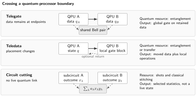
Three distinct boundary mechanisms. A telegate keeps data at their endpoints and consumes entanglement for a nonlocal operation. Teledata changes quantum state placement before local work. Circuit cutting uses no live quantum link; weighted classical reconstruction combines repeated subcircuit outcomes.

Telegate

A telegate uses preshared entanglement, local operations, measurements, classical communication, and feed-forward to implement a gate whose operands remain in separate modules. The term overlaps with gate teleportation, but that phrase is broader: it also includes teleporting data through a specially prepared resource state to implement a difficult local gate. Here telegate means a nonlocal operation between QPUs.

The network can prepare a Bell pair before the application reaches the gate. Photon loss then causes another resource-generation attempt rather than loss of the data qubits. The gate is deterministic only conditioned on an accepted pair and successful required local operations. Calling the entire service deterministic while omitting stochastic setup time is misleading.

Teledata

Teledata moves a data state from one QPU to another, usually by quantum teleportation. Gates that were nonlocal can then be executed locally. The source qubit is consumed and the destination qubit takes over its logical identity; the compiler’s placement map must change.

Teledata can save entanglement when one qubit participates in many operations at a remote module. It can also create later communication, overload the destination, or require a return teleport. State placement is therefore a time-dependent compilation decision rather than a one-time graph partition.

Circuit cutting

Circuit cutting replaces a wire or nonlocal gate by a linear combination of local preparations, operations, and measurements. The subcircuits can run without a quantum link, after which a classical estimator reconstructs a specified quantity. The price is often exponential sampling or term-count overhead in the number and kind of cuts. It is not a free substitute for entanglement-assisted execution.

Remote CNOT from One Bell Pair

The remote controlled-NOT is the basic telegate because it exposes every architectural ingredient. Alice holds control $c$ and one half $a$ of

$$\lvert\Phi^+\rangle_{ab} = \frac{\lvert00\rangle_{ab}+\lvert11\rangle_{ab}}{\sqrt2},$$

while Bob holds $b$ and target $t$. The arbitrary data state is

$$\lvert\psi\rangle_{ct} = \sum_{i,j\in\{0,1\}} \alpha_{ij} \lvert i\rangle_c\lvert j\rangle_t.$$

Entangle the remote control

Alice applies $\operatorname{CNOT}_{c\to a}$, measures $a$ in the computational basis, and sends outcome $m\in\{0,1\}$ to Bob. Bob applies $X_b^m$, physically or through an equivalent frame update. Up to normalization, the surviving state is

$$\lvert\Psi_1\rangle_{cbt} = \sum_{i,j} \alpha_{ij} \lvert i\rangle_c \lvert i\rangle_b \lvert j\rangle_t.$$

The control information is now encoded nonlocally in a two-qubit cat state. Alice has not measured $c$, so superpositions and entanglement with a reference are preserved.

Apply the target operation locally

Bob applies $\operatorname{CNOT}_{b\to t}$:

$$\lvert\Psi_2\rangle_{cbt} = \sum_{i,j} \alpha_{ij} \lvert i\rangle_c \lvert i\rangle_b \lvert j\oplus i\rangle_t.$$

He then measures $b$ in the $X$ basis. Let $n=0$ denote outcome $\lvert+\rangle$ and $n=1$ denote $\lvert-\rangle$. The data qubits become

$$\lvert\psi_n\rangle_{ct} = Z_c^n \sum_{i,j} \alpha_{ij} \lvert i\rangle_c \lvert j\oplus i\rangle_t.$$

Bob sends $n$ to Alice, who applies $Z_c^n$ or updates the Pauli frame. Since $(Z_c^n)^2=I$, the result is

$$\lvert\psi_{\rm out}\rangle_{ct} = \operatorname{CNOT}_{c\to t} \lvert\psi\rangle_{ct}.$$

The protocol consumes one ebit, uses one local CNOT in each module, measures the two network qubits, and sends one classical bit in each direction. These resources are necessary and sufficient for exact deterministic remote CNOT under the standard LOCC setting. A remote controlled-$Z$ follows from

$$\operatorname{CZ}_{ct} = (I_c\otimes H_t) \operatorname{CNOT}_{c\to t} (I_c\otimes H_t).$$

The two classical messages enforce causality. Before they arrive, the local reduced states do not give either party the completed gate. Feed-forward can often be tracked in software, but a later non-Clifford operation or measurement may require the frame to be resolved.

Teledata versus Telegate

There is no universal winner. Consider a qubit at Alice that must control $k$ gates on Bob’s data and eventually return to Alice. A naive telegate lowering uses $k$ Bell pairs. Teledata can teleport the qubit to Bob, perform all $k$ gates locally, and teleport it back, using two Bell pairs. If the final state may remain at Bob, it uses only one.

This count is an orientation, not an optimizer. It omits:

• whether Bob has a free data and communication port;
• operations on Alice’s qubit that must occur between remote gates;
• Bell-pair fidelity, age, and directional classical latency;
• the cost of updating every later reference to the migrated logical qubit;
• parallel remote gates that telegate can execute while one teledata transfer serializes a path;
• fault-tolerant code deformation, decoding, or logical teleportation.

Repeated controlled operations can sometimes be packed into one entanglement-assisted distributing process. The cat-like remote-control state is retained across several compatible target operations and disentangled only afterward. Incompatible intervening gates or causality constraints break the packing. Counting every syntactically nonlocal CNOT as one ebit is therefore a constructive upper bound, not always the optimum.

For each candidate remote block $B$, a compiler should compare a resource vector rather than just Bell-pair count:

$$\mathbf c(B) = \left( N_{\rm ebit}, B_{A\to B},B_{B\to A}, T_{\rm crit}, n_{\rm anc}, p_{\rm fail}, \varepsilon_B \right).$$

An ebit-saving transformation can lose overall if it lengthens the critical path beyond memory lifetime or raises correlated error.

Partitioning the Program

Weighted interaction graph

For a circuit on logical qubits $Q$, define a weighted interaction graph $G_C=(Q,E_C,w)$. A simple weight is the number of two-qubit gates between $q_i$ and $q_j$,

$$w_{ij} = \sum_{g\in\mathcal G_2} \mathbf 1 \left[ g\text{ acts on }(q_i,q_j) \right].$$

For a static placement $\pi:Q\to\{1,\ldots,M\}$, the naive cut cost is

$$C_{\rm cut}(\pi) = \sum_{(i,j)\in E_C} w_{ij} \mathbf 1[\pi(q_i)\ne\pi(q_j)].$$

Minimizing this cost subject to each QPU’s capacity is a useful first step. It is not the complete compilation problem. Gates have a causal order; Bell pairs can be packed or generated in parallel; links and network ports have unequal rate; QPUs have different native gates and error; and a low-cut partition can create a long serial bottleneck.

Why hypergraphs help

Several nonlocal controlled gates that share a control can sometimes use one distributed control state. Representing that group as a hyperedge captures a resource that pairwise edge counting misses. Hypergraph partitioning has therefore been used to group circuit structure while minimizing quantum communication. The hyperedge weight must still correspond to a realizable remote protocol; a combinatorial grouping is not itself a schedule.

Time-dependent placement

With teledata, the placement is $\pi_t(q)$ rather than a fixed map. Moving a qubit can make a future block local and a formerly local block remote. A time-expanded compiler can choose migrations, telegates, and local SWAPs while respecting QPU and link capacity.

A schematic objective is

$$\begin{aligned} \text{minimize}\quad & \alpha N_{\rm ebit} +\beta T_{\rm makespan} +\gamma P_{\rm fail} +\delta N_{\rm move},\\ \text{subject to}\quad & n_i(t)\le n_i^{\max},\\ & u_e(t)\le C_e(t),\\ & \text{program dependencies and deadlines}. \end{aligned}$$

The coefficients express policy and units; they do not turn incomparable quantities into a physical law. In practice one may seek a Pareto frontier or constrain error and deadline while minimizing resources.

Distributed Compilation and Runtime

A complete toolchain has at least the following responsibilities.

1. Normalize semantics. Express dynamic control, measurement outcomes, resets, and required output placement explicitly.
2. Characterize the target. Load local gate, memory, network-port, entanglement-service, latency, error, and trust capabilities.
3. Partition and place. Assign initial data and ancillas while minimizing expensive boundary structure under capacity constraints.
4. Select boundary primitives. Choose direct transfer, teledata, telegate, distributed measurement, packed blocks, or circuit cutting.
5. Plan entanglement. Request pair count, endpoints, quality, deadline, reservation, and renewal policy from the network layer.
6. Compile locally. Map each subprogram to its QPU without erasing global causal dependencies or frame information.
7. Schedule globally. Coordinate Bell-pair availability, network ports, local gates, measurement, classical messages, and memory leases.
8. Execute and recover. Correlate request and pair identifiers, resolve frames, handle timeouts, and make partial failure atomic at the program level.
9. Validate the result. Report application success, not only local gate fidelity or elementary-pair rate.

The compiler produces a distributed dependency graph. An operation becomes ready only when its local data, remote resources, classical prerequisites, and lease margins are all valid. A Pauli correction need not always stall the machine: Clifford operations can propagate a known frame. But the frame must remain attached to the correct logical qubit after teledata movement and cannot be discarded merely because no physical pulse was applied.

Runtime interfaces such as NetQASM and QNodeOS demonstrate how high-level network applications, node processes, and entanglement requests can be separated from hardware drivers. They do not remove the compiler’s need to know performance contracts, and they do not establish that arbitrary heterogeneous QPUs already share one portable fault-tolerant instruction set.

Latency, Throughput, and Backpressure

For one remote gate admitted only after a usable Bell pair exists, write

$$T_{\rm remote} = T_{\rm wait}^{\rm Bell} +T_{\rm local} +T_{\rm meas} +T_{\rm class} +T_{\rm ff}.$$

If a valid pair was generated proactively and reserved in advance, $T_{\rm wait}^{\rm Bell}$ can be hidden from that gate’s observed latency. It has not vanished from resource cost: the inventory occupies memories, decoheres, and may expire unused.

For an execution dependency graph $D=(O,E_D)$ with duration $d_o$ for each operation, the ideal makespan obeys the critical-path lower bound

$$T_{\rm run} \ge \max_{P\in\operatorname{Paths}(D)} \sum_{o\in P}d_o.$$

Resource contention can make the actual value larger. Two causally independent remote gates may still serialize on one network qubit, detector, switch, Bell source, or classical controller.

If an application consumes on average $\bar e$ accepted Bell pairs per run, then a basic steady-state constraint is

$$R_{\rm app} \le \frac{R_{\rm Bell}^{\rm accepted}}{\bar e}.$$

The accepted rate must use the application’s quality and age thresholds. A more complete bottleneck bound includes local gates, measurements, decoder capacity, and the narrowest network cut:

$$R_{\rm app} \le \min \left( \frac{R_{\rm Bell}}{\bar e}, \frac{R_{\rm local}}{\bar g}, \frac{R_{\rm meas}}{\bar m}, R_{\rm dec}, R_{\rm cut} \right).$$

Average demand is insufficient for bursty circuits. If a layer needs $b$ pairs nearly simultaneously but a module buffers only $m<b$, the scheduler must split the layer or change the primitive. Local QPUs then experience backpressure while waiting for network supply. Queueing delay lengthens memory exposure and can raise the number of pairs discarded by age cutoffs.

Noise and Correctness

Compose channels, not slogans

A noisy remote operation includes Bell-state preparation, storage, local gates, measurements, classical decoding, and corrections. If each implemented component channel $\widetilde{\mathcal E}_j$ is compared with an ideal $\mathcal E_j$ by

$$\epsilon_j = \frac12 \left\| \widetilde{\mathcal E}_j-\mathcal E_j \right\|_\diamond,$$

then repeated triangle inequalities give the conservative compositional bound

$$\epsilon_{\rm remote} \le \sum_j\epsilon_j.$$

This bound can be loose, but it has a valid operational meaning. Adding incompatible state fidelities as though they were independent error probabilities does not.

Heralded loss and false heralds

Loss before admission can be retried if failed attempts leave data intact. A false herald is more dangerous: the runtime admits a remote operation while the advertised resource is absent or wrong. Report conditional pair quality, false-herald probability, data disturbance during failed attempts, and the full wait distribution separately.

Correlated and non-Pauli errors

The same optical phase, clock, calibration, or controller can affect several remote gates. Leakage can persist between operations. Pair purification can correlate accepted resources through shared data. A stochastic independent Pauli model is useful only after its adequacy has been tested for the workload and decoder.

What “deterministic” means

At least four probabilities may be present:

$$p_{\rm app} = p_{\rm resource} p_{\rm admit} p_{\rm gate\mid admit} p_{\rm accept\mid gate}.$$

A gate-teleportation protocol can have $p_{\rm gate\mid admit}=1$ ideally while $p_{\rm resource}\ll1$ per optical attempt. Postselecting successful tomography adds another acceptance condition. State which probability a reported success rate describes.

Circuit Cutting and Classical Reconstruction

Suppose a nonlocal channel or wire segment is represented by a signed linear combination

$$\mathcal E_{AB} = \sum_{\lambda=1}^{L} a_\lambda \mathcal A_\lambda\otimes\mathcal B_\lambda,$$

where the local terms can be implemented by subcircuits, possibly with measurement-conditioned instruments and classical communication. Then an observable can be reconstructed as

$$\langle O_A\otimes O_B\rangle = \sum_{\lambda=1}^{L} a_\lambda \mathbb E_\lambda[o_Ao_B].$$

Because some $a_\lambda$ are negative, this is a quasiprobability estimator, not a physical mixture. Define

$$\gamma = \sum_\lambda |a_\lambda|.$$

Sampling term $\lambda$ with probability $p_\lambda=|a_\lambda|/\gamma$ gives a single-shot weight proportional to $\gamma\operatorname{sgn}(a_\lambda)$. For bounded outcomes, the number of shots needed for fixed additive precision scales at least schematically as

$$N_{\rm shots} = O\!\left( \frac{\gamma^2}{\epsilon^2} \log\frac1\delta \right),$$

where $\epsilon$ is estimator error and $1-\delta$ the confidence level. For independently cut components, the total $\gamma$ often multiplies, producing exponential overhead in cut count. Joint decompositions can be cheaper than cutting each gate separately, so a raw number of cut wires is not a universal cost metric.

Circuit cutting is attractive when:

• only selected observables or marginal probabilities are required;
• the circuit has a weak, low-rank boundary;
• subcircuits fit substantially better on available hardware;
• classical postprocessing and repeated shots are cheaper than a quantum link;
• noise reduction from smaller subcircuits outweighs reconstruction variance.

It is unattractive when many cuts multiply $\gamma$, the full output distribution is required, or a later quantum stage needs the joint output state. Report number and type of cuts, decomposition norm, term count, shots, classical postprocessing, error bars, and any noise-mitigation bias. “Ran a larger circuit” is incomplete if only one reconstructed observable was obtained.

Fault-Tolerant Distributed Computing

Physical remote gates are not enough for long algorithms. Fault-tolerant DQC must connect logical qubits while keeping link errors, waiting, and classical latency inside a correctable spacetime fault model.

Several architecture families are under study:

• purify noisy physical Bell pairs before injecting them into logical operations;
• prepare encoded Bell pairs and use logical teleportation;
• measure nonlocal logical parities through shared Bell resources and lattice surgery;
• apply transversal remote gates between compatible code blocks;
• build a distributed cluster or graph state and compute by measurements.

The network requirement is code- and schedule-dependent. “Bell fidelity above threshold” is not a standalone criterion. The operation may need a burst of many pairs per code cycle, correlated failures can defeat a decoder, and slow delivery can enlarge the spacetime volume exposed to memory error.

A logical resource ledger should include

$$\mathcal R_L = \left( d, N_{\rm phys/QPU}, N_{\rm Bell/cycle}, F_{\rm Bell}, t_{\rm cycle}, p_L, N_{\rm factories}, T_{\rm decode} \right),$$

where $d$ is code distance and $p_L$ is the logical failure probability under the complete model. Different codes and remote primitives trade network rate, local qubits, decoder complexity, and logical latency.

Recent circuit-level studies illustrate the scale of the assumptions. A 2026 surface-code resource estimate found negligible modeled overhead relative to its monolithic reference only when each processor boundary supplied tens of high-fidelity Bell pairs per microsecond-scale cycle. A separate 2026 study simulated transversal nonlocal CNOT and logical teleportation for surface and bivariate-bicycle codes and found architecture-dependent advantages. These are valuable model results, not experimental demonstrations of distributed fault-tolerant algorithms.

Workloads and When Distribution Helps

Distribution is most plausible when it relieves a binding physical constraint: fabrication yield, cryogenic wiring, optical access, local connectivity, control crosstalk, or maximum code-block size. It can also connect specialized modules such as data processors, memories, magic-state factories, and photonic interfaces.

The workload must have exploitable structure. Examples include:

• arithmetic with blocks that interact through narrow carry interfaces;
• Hamiltonian simulation with weakly coupled spatial or orbital fragments;
• algorithms whose control qubits can support packed remote controlled gates;
• fault-tolerant factories that feed several data modules;
• circuits whose interaction graph follows a sparse module graph;
• ensembles of subproblems whose classical outer loop is naturally parallel.

No generic complexity advantage follows from replacing one $n$-qubit QPU by two $n/2$-qubit QPUs. The joint Hilbert space has the same formal dimension only if the network operations preserve coherent access to it. Communication can dominate runtime, error, or qubit overhead. For classically separable workloads, independent QPUs may improve throughput without increasing the largest coherent problem size.

Geographic distance is often a disadvantage for tightly coupled computation because classical round trips enter the critical path. A modular machine under one scheduler and a federation across administrative domains may use the same remote-CNOT identity but have very different latency, trust, calibration, and failure contracts.

Security, Ownership, and Recovery

Distributed execution expands the trusted computing base. The system must authenticate program fragments, pair and request identifiers, measurement messages, calibration versions, and result provenance. A malicious QPU can return plausible but false outcomes; a compromised controller can alter placement or route sensitive metadata through an unauthorized domain.

Ordinary fault recovery and adversarial verification are different:

• a crash fault can trigger timeout, pair cleanup, and rescheduling if the program state has not been irreversibly consumed;
• a Byzantine or malicious fault requires cryptographic or quantum verification, often with substantial overhead;
• a straggler can hold entanglement and memory leases while other QPUs decohere;
• a partial commit can consume one side of a resource while another node retries unless operation identifiers and state transitions are atomic.

Blindness, verifiability, and secure multiparty computation require dedicated protocols. Entanglement alone does not hide a circuit, input, output, timing, or communication graph.

Experimental and Evidence Status

Evidence should be labeled by the strongest complete boundary crossed.

1. Remote primitive: a nonlocal gate or state transfer is characterized between separated qubits.
2. Repeatable instruction: the primitive can be invoked more than once while retained data remain usable.
3. Distributed circuit: several local and nonlocal gates execute one program with feed-forward and an application output.
4. Scalable runtime: compilation, reservation, scheduling, recovery, and concurrent workload are automated.
5. Fault-tolerant DQC: encoded operations reduce logical error with scale under a complete end-to-end resource ledger.

The 2019 trapped-ion gate-teleportation experiment implemented a CNOT between separated zones of one processor with real-time feed-forward. The 2021 atom–photon experiment implemented a heralded nonlocal gate between modules separated by $60\ \mathrm{m}$. Both established important remote primitives, with different physical and admission semantics.

In 2025, Main and co-workers connected two trapped-ion modules over an optical link, buffered heralded network-qubit entanglement, teleported a controlled-$Z$ between circuit qubits, repeated the operation in distributed iSWAP and SWAP circuits, and ran a two-qubit Grover search. The reported controlled-$Z$ fidelity was $86\%$ and the Grover success rate $71\%$. This is evidence for a small distributed processor, not for fault-tolerant or throughput-improving scale-out.

Also in 2025, QNodeOS demonstrated high-level network applications and multitasking on a two-node NV-center system, with a separate trapped-ion driver integration. That advances runtime abstraction, but it does not establish one portable, fault-tolerant distributed-computing stack across heterogeneous nodes.

For every DQC claim, report:

• physical separation and whether modules share vacuum, clock, controller, source, or calibration;
• data, network, ancilla, and logical qubit counts;
• remote-operation protocol and entanglement consumed;
• Bell attempt, accepted-pair, admitted-gate, and application denominators;
• local, remote, memory, measurement, and feed-forward error evidence;
• latency distribution, pair age, duty factor, and classical round trips;
• compiler partition, remote-operation count, schedule, and baselines;
• wall-clock application success with confidence intervals;
• which components were measured, simulated, assumed, or projected.

Common Mistakes

Equating aggregate qubits with coherent capacity

Two disconnected 50-qubit QPUs are not a 100-qubit coherent processor. The cross-QPU operations and their resource budget determine which 100-qubit channels can actually be implemented.

Calling independent shots DQC

Shot parallelism improves throughput but does not demonstrate a state or gate spanning processors. Label it as parallel execution unless quantum data or entanglement couples the subprograms.

Treating teleportation as free movement

Teledata consumes entanglement, two classical bits per qubit teleport, endpoint memories, Bell measurements, feed-forward, and time. It also changes logical placement.

Counting every cut edge as one ebit without qualification

Packed telegates can share an entanglement resource, while fault-tolerant gates can consume many physical or logical pairs. Translate graph cuts into actual protocol blocks.

Ignoring Bell-pair setup in “deterministic” gates

A remote gate can be deterministic after admission while pair generation is probabilistic. Report both the conditional gate success and wall-clock service rate.

Treating circuit cutting as a coherent quantum link

Classical reconstruction can estimate selected outputs, but it does not in general produce the live joint state needed by a later quantum stage. Include the quasiprobability and shot overhead.

Comparing local and remote fidelities with different conventions

State fidelity, average gate fidelity, process fidelity, Bell-state fidelity, and logical failure probability are not interchangeable. Use a matched channel or application metric.

Assuming distribution supplies privacy or fault tolerance

Privacy requires a security protocol, and fault tolerance requires encoded operations whose errors decrease under a validated model. Physical separation provides neither by itself.

Exercises

Exercise 1: Verify the remote CNOT

Start with

$$\lvert\psi\rangle_{ct} = \alpha\lvert00\rangle +\beta\lvert01\rangle +\gamma\lvert10\rangle +\delta\lvert11\rangle.$$

Using the protocol above, write the final state before Alice’s last $Z^n$ correction and then after it.

Solution

After the cat-entangler, Bob’s local CNOT, and his $X$-basis measurement with outcome $n$, the data state is

$$\begin{aligned} \lvert\psi_n\rangle_{ct} ={}& \alpha\lvert00\rangle +\beta\lvert01\rangle\\ &+(-1)^n\gamma\lvert11\rangle +(-1)^n\delta\lvert10\rangle. \end{aligned}$$

This is $Z_c^n\operatorname{CNOT}\lvert\psi\rangle$. Alice’s correction $Z_c^n$ cancels the phase, giving

$$\alpha\lvert00\rangle +\beta\lvert01\rangle +\gamma\lvert11\rangle +\delta\lvert10\rangle,$$

which is exactly $\operatorname{CNOT}_{c\to t}\lvert\psi\rangle$.

Exercise 2: Teledata or telegate?

A qubit at $A$ must control five compatible gates on data at $B$ and then be used again at $A$. Compare the naive Bell-pair counts for telegate and for teledata. State two reasons the lower count need not minimize runtime.

Solution

Naive telegate lowering uses one Bell pair per remote controlled gate, for five pairs. Teledata sends the control to $B$, performs five local gates, and returns it to $A$, for two teleportations and therefore two Bell pairs. It also uses four classical bits in the teleportation directions.

The two-pair strategy can still be slower if the transfers serialize on a network port, while telegates could use parallel links or pregenerated pairs. It may also wait for a free destination data slot, incur more logical movement or code deformation, or disrupt operations at $A$. Conversely, compatible telegates might themselves be packed into fewer than five pairs, so the naive count is not optimal.

Exercise 3: Weighted partition

Four logical qubits have interaction weights

$$w_{12}=8, \quad w_{23}=3, \quad w_{34}=8, \quad w_{14}=1, \quad w_{13}=2.$$

Two equal QPUs each hold two qubits. Compute the cut cost for the three distinct balanced partitions and choose the best under the naive objective.

Solution

For $\{1,2\}|\{3,4\}$, the crossing edges are $(2,3)$, $(1,4)$, and $(1,3)$, so

$$C_{\rm cut}=3+1+2=6.$$

For $\{1,4\}|\{2,3\}$, edges $(1,2)$, $(3,4)$, and $(1,3)$ cross, giving $8+8+2=18$. For $\{1,3\}|\{2,4\}$, edges $(1,2)$, $(2,3)$, $(3,4)$, and $(1,4)$ cross, giving $8+3+8+1=20$. The first partition is best under this static edge-count model. Rate, packing, port contention, and gate order can change the preferred executable schedule.

Exercise 4: Hiding pair-generation latency

Accepted Bell-pair waiting time has mean $40\ \mathrm{ms}$, while local gates, measurement, classical messaging, and feed-forward take $1\ \mathrm{ms}$. Find the mean observed gate latency for reactive generation. If proactive inventory supplies a valid pair on arrival with probability $0.8$, and a miss then incurs the full reactive latency, find the simplified mean.

Solution

Reactive execution has mean

$$\mathbb E[T_{\rm reactive}] = 40+1 = 41\ \mathrm{ms}.$$

With an inventory hit, the gate takes $1\ \mathrm{ms}$; with a miss, it takes $41\ \mathrm{ms}$. Thus

$$\mathbb E[T_{\rm proactive}] = 0.8(1)+0.2(41) = 9\ \mathrm{ms}.$$

The improvement consumes memory time and generation capacity and ignores pair expiration, replacement policy, and correlations in demand.

Exercise 5: Circuit-cutting overhead

Suppose each of four independent gate cuts has quasiprobability norm $\gamma_0=3$. Estimate the product norm and the relative shot-overhead factor $\gamma^2$ compared with an estimator of norm one.

Solution

Independent decompositions multiply:

$$\gamma = \gamma_0^4 = 3^4 =81.$$

The variance-driven shot factor is therefore

$$\gamma^2 = 81^2 =6561.$$

This illustrates exponential cut cost. A joint decomposition can have a lower norm, and real shot cost also depends on observable variance, allocation among terms, confidence, hardware noise, and postprocessing.

Exercise 6: Compositional error bound

A remote gate has diamond-distance bounds $0.004$ for its Bell resource, $0.001$ for Alice’s local block, $0.002$ for Bob’s block, and $0.003$ for measurement and feed-forward. Give the conservative composed bound and explain why it need not predict measured average gate infidelity.

Solution

The triangle bound gives

$$\epsilon_{\rm remote} \le 0.004+0.001+0.002+0.003 =0.010.$$

Diamond distance is a worst-case channel metric, including reference-system entanglement. Average gate infidelity averages over inputs and has a dimension-dependent relation to channel distances. Coherent errors can also combine constructively or cancel. The number $0.010$ is a valid conservative bound under the component contracts, not a prediction that tomography must report one percent infidelity.

Exercise 7: Logical Bell-pair supply

A transversal remote logical operation on distance-$7$ blocks consumes seven qualified physical Bell pairs simultaneously. The workload requests $200$ such operations per second. What accepted pair rate and burst buffer are necessary before retries? If purification yield is $0.20$, what raw pair rate is required in the simplified steady-state model?

Solution

The accepted demand is

$$R_{\rm Bell}^{\rm accepted} = 7\times200 =1400\ \mathrm{s}^{-1}.$$

At least seven compatible pairs must be available together for one operation, so a buffer of one or two pairs cannot sustain the stated primitive even if its long-term average rate is high. With yield $Y=0.20$,

$$R_{\rm Bell}^{\rm raw} = \frac{1400}{0.20} =7000\ \mathrm{s}^{-1}.$$

Actual provisioning must include failed logical operations, age cutoffs, quality correlations, and headroom for burst and outage statistics.

Exercise 8: Audit a scale-out claim

A team runs 100 independent parameter points on ten 20-qubit processors and states that it demonstrated a 200-qubit distributed quantum computer. Rewrite the strongest supported claim. What additional evidence would support a coherent 200-qubit claim?

Solution

The supported claim is that ten 20-qubit processors executed a classically parallel ensemble of 100 circuit instances, with whatever throughput and quality the report establishes. The largest demonstrated coherent register is at most 20 qubits unless a cross-QPU quantum operation was used.

A coherent 200-qubit claim would require declared state-transfer or entanglement-assisted operations linking all participating QPUs, a compiled global circuit whose state crosses those boundaries, end-to-end channel or application validation, remote-operation and classical-control ledgers, latency and fidelity evidence, and proof that postselection or classical reconstruction did not replace the claimed live joint state.

References

1. D. Gottesman and I. L. Chuang, “Demonstrating the viability of universal quantum computation using teleportation and single-qubit operations,” Nature 402, 390–393 (1999), doi:10.1038/46503.
2. J. Eisert, K. Jacobs, P. Papadopoulos, and M. B. Plenio, “Optimal local implementation of nonlocal quantum gates,” Physical Review A 62, 052317 (2000), doi:10.1103/PhysRevA.62.052317.
3. R. Van Meter, K. Nemoto, W. J. Munro, and K. M. Itoh, “Distributed Arithmetic on a Quantum Multicomputer,” Proceedings of the 33rd International Symposium on Computer Architecture, 354–365 (2006), doi:10.1145/1150019.1136517.
4. L. Jiang, J. M. Taylor, A. S. Sørensen, and M. D. Lukin, “Distributed quantum computation based on small quantum registers,” Physical Review A 76, 062323 (2007), doi:10.1103/PhysRevA.76.062323.
5. C. Monroe et al., “Large-scale modular quantum-computer architecture with atomic memory and photonic interconnects,” Physical Review A 89, 022317 (2014), doi:10.1103/PhysRevA.89.022317.
6. N. H. Nickerson, J. F. Fitzsimons, and S. C. Benjamin, “Freely scalable quantum technologies using cells of 5-to-50 qubits with very lossy and noisy photonic links,” Physical Review X 4, 041041 (2014), doi:10.1103/PhysRevX.4.041041.
7. P. Andrés-Martínez and C. Heunen, “Automated distribution of quantum circuits via hypergraph partitioning,” Physical Review A 100, 032308 (2019), doi:10.1103/PhysRevA.100.032308.
8. D. Cuomo, M. Caleffi, and A. S. Cacciapuoti, “Towards a distributed quantum computing ecosystem,” IET Quantum Communication 1, 3–8 (2020), doi:10.1049/iet-qtc.2020.0002.
9. D. Ferrari, A. S. Cacciapuoti, M. Amoretti, and M. Caleffi, “Compiler Design for Distributed Quantum Computing,” IEEE Transactions on Quantum Engineering 2, 1–20 (2021), doi:10.1109/TQE.2021.3053921.
10. D. Ferrari, S. Carretta, and M. Amoretti, “A Modular Quantum Compilation Framework for Distributed Quantum Computing,” IEEE Transactions on Quantum Engineering 4, 1–13 (2023), doi:10.1109/TQE.2023.3303935.
11. J.-Y. Wu et al., “Entanglement-efficient bipartite-distributed quantum computing,” Quantum 7, 1196 (2023), doi:10.22331/q-2023-12-05-1196.
12. T. Peng, A. W. Harrow, M. Ozols, and X. Wu, “Simulating Large Quantum Circuits on a Small Quantum Computer,” Physical Review Letters 125, 150504 (2020), doi:10.1103/PhysRevLett.125.150504.
13. C. Piveteau and D. Sutter, “Circuit Knitting With Classical Communication,” IEEE Transactions on Information Theory 70, 2734–2745 (2024), doi:10.1109/TIT.2023.3310797.
14. L. Schmitt, C. Piveteau, and D. Sutter, “Cutting circuits with multiple two-qubit unitaries,” Quantum 9, 1634 (2025), doi:10.22331/q-2025-02-18-1634.
15. Y. Wan et al., “Quantum gate teleportation between separated qubits in a trapped-ion processor,” Science 364, 875–878 (2019), doi:10.1126/science.aaw9415.
16. S. Daiss et al., “A quantum-logic gate between distant quantum-network modules,” Science 371, 614–617 (2021), doi:10.1126/science.abe3150.
17. D. Main et al., “Distributed quantum computing across an optical network link,” Nature 638, 383–388 (2025), doi:10.1038/s41586-024-08404-x.
18. A. Dahlberg et al., “NetQASM—a low-level instruction set architecture for hybrid quantum–classical programs in a quantum internet,” Quantum Science and Technology 7, 035023 (2022), doi:10.1088/2058-9565/ac753f.
19. C. Delle Donne et al., “An operating system for executing applications on quantum network nodes,” Nature 639, 321–328 (2025), doi:10.1038/s41586-025-08704-w.
20. H. Jacinto, É. Gouzien, and N. Sangouard, “Network requirements for distributed quantum computation,” Physical Review Research 8, 013205 (2026), doi:10.1103/v9ln-c4v2.
21. J. Stack, M. Wang, and F. Mueller, “Transversal fault tolerant distributed quantum computing operations,” Nature Communications (2026), doi:10.1038/s41467-026-75693-3.
22. F. Burt, K.-C. Chen, and K. K. Leung, “A Multilevel Framework for Partitioning Quantum Circuits,” Quantum 10, 1984 (2026), doi:10.22331/q-2026-01-22-1984.