Entanglement Swapping

Entanglement swapping consumes two neighboring entangled links and performs a joint measurement on their middle systems so that the unmeasured endpoints become entangled, conditioned on the measurement record. The endpoints need not have interacted, shared a source, or exchanged a quantum system directly.

The word conditioned is essential. In the ideal qubit protocol, a Bell measurement produces one of four two-bit outcomes. Given that outcome, the endpoints share a known Bell state. If the outcome is ignored, their averaged state is maximally mixed and separable.

This page is the canonical home for the swapping identity, circuit-level protocol, Pauli-frame record, nonideal input analysis, success accounting, and interpretation. Entanglement Sharing owns the broader distinction among pairwise, global, and localizable entanglement and the associated cut structure. Network Case Studies owns evidence-led comparisons of physical demonstrations and end-to-end network services.

Protocol Contract

Four qubit registers are involved:

• $A$ and $B$ share one Bell pair;
• $C$ and $D$ share a second Bell pair;
• a middle station can jointly measure $B$ and $C$;
• $A$ and $D$ are the remote endpoint registers.

For the ideal protocol, the initial state is

$$|\Omega\rangle_{ABCD} = |\Phi^+\rangle_{AB} \otimes |\Phi^+\rangle_{CD},$$

where

$$|\Phi^+\rangle = \frac{|00\rangle+|11\rangle}{\sqrt2}.$$

The middle station performs a complete Bell-basis measurement on $BC$ and records two classical bits $(a,b)$. The output contract is:

1. the measurement succeeds and returns $(a,b)$;
2. conditioned on that record, $AD$ is in a known Bell state;
3. an endpoint may apply a Pauli correction, or track a Pauli frame, to use a fixed target state;
4. the original $AB$ and $CD$ links are consumed.

In compact resource language,

$$\begin{gathered} 2\ \text{neighboring ebits} + 1\ \text{Bell measurement} \\ \longrightarrow 1\ \text{longer-range ebit} + 2\ \text{classical record bits}, \end{gathered}$$

conditioned on a successful measurement. This is a conversion rule, not an entanglement amplifier: two elementary pairs are consumed to obtain at most one endpoint pair.

For a physical analyzer that succeeds only probabilistically, the contract must also include a heralding flag $s$ and its probability $p_{\mathrm{swap}}=\Pr(s=1)$. Fidelity conditioned on $s=1$ and rate per attempt are different performance quantities.

Bell-Basis Identity

Use the same phase-bit and parity-bit convention as in Superdense Coding:

$$|\beta_{ab}\rangle = (Z^aX^b\otimes I)|\Phi^+\rangle, \qquad a,b\in\{0,1\}.$$

Thus

$$\begin{array}{ccl} |\beta_{00}\rangle&=&|\Phi^+\rangle,\\ |\beta_{10}\rangle&=&|\Phi^-\rangle,\\ |\beta_{01}\rangle&=&|\Psi^+\rangle,\\ |\beta_{11}\rangle&=&|\Psi^-\rangle. \end{array}$$

Regrouping the four-register state by the middle pair $BC$ and endpoint pair $AD$ gives the swapping identity

$$|\Phi^+\rangle_{AB} |\Phi^+\rangle_{CD} = \frac12 \sum_{a,b=0}^{1} |\beta_{ab}\rangle_{BC} |\beta_{ab}\rangle_{AD}.$$

This identity is a change of basis, not a new dynamical law. To verify it, expand the left-hand side:

$$\begin{aligned} |\Omega\rangle = \frac12\bigl( &|0\rangle_A|0\rangle_B|0\rangle_C|0\rangle_D \\ &+ |0\rangle_A|0\rangle_B|1\rangle_C|1\rangle_D \\ &+ |1\rangle_A|1\rangle_B|0\rangle_C|0\rangle_D \\ &+ |1\rangle_A|1\rangle_B|1\rangle_C|1\rangle_D \bigr). \end{aligned}$$

The equal-parity terms can be rewritten with $|00\rangle=(|\Phi^+\rangle+|\Phi^-\rangle)/\sqrt2$ and $|11\rangle=(|\Phi^+\rangle-|\Phi^-\rangle)/\sqrt2$. The odd-parity terms use the analogous relations for $|\Psi^\pm\rangle$. Cross terms cancel, leaving equal Bell labels on $BC$ and $AD$.

Conditional projection

Let

$$P_{ab}^{BC} = |\beta_{ab}\rangle\langle\beta_{ab}|_{BC}.$$

The probability of outcome $(a,b)$ is

$$\begin{aligned} p_{ab} &= \langle\Omega| \bigl( I_A\otimes P_{ab}^{BC}\otimes I_D \bigr) |\Omega\rangle \\ &= \frac14. \end{aligned}$$

After normalization, the endpoint state is

$$\rho_{AD|ab} = |\beta_{ab}\rangle \langle\beta_{ab}|_{AD}.$$

The four cases are therefore:

outcome $(a,b)$	measured state on $BC$	conditional state on $AD$	inverse endpoint frame
$(0,0)$	$	\Phi^+\rangle$	$
$(1,0)$	$	\Phi^-\rangle$	$
$(0,1)$	$	\Psi^+\rangle$	$
$(1,1)$	$	\Psi^-\rangle$	$

Applying $(Z^aX^b)^\dagger=X^bZ^a$ to the first endpoint converts the conditional state to $|\Phi^+\rangle$, up to an irrelevant global phase. Many network stacks do not apply this correction immediately. They store $(a,b)$ in a Pauli frame and reinterpret later Clifford operations or measurement outcomes.

Measurement Circuit and Network View

A complete Bell measurement can be implemented abstractly with an inverse Bell transform:

1. apply $\operatorname{CNOT}_{B\to C}$;
2. apply $H_B$;
3. measure $B$ and $C$ in the computational basis.

The first measurement bit is the phase label $a$ and the second is the parity label $b$ under the convention above.

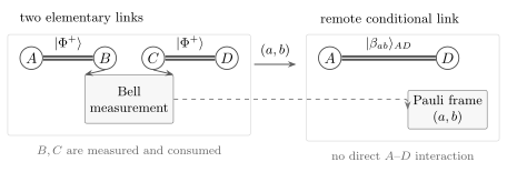
Operational view of entanglement swapping. The $AB$ and $CD$ links are consumed by a Bell measurement on $BC$. Conditioned on the classical record $(a,b)$, the untouched endpoints share $|\beta_{ab}\rangle_{AD}$; the record can be used as a Pauli-frame update rather than an immediate physical gate.

The circuit is deterministic when the platform provides a deterministic two-qubit entangling gate and reliable measurements. A photonic Bell analyzer may instead identify only a subset of Bell outcomes. The abstract protocol and the physical analyzer must therefore be kept separate.

Why the Classical Record Matters

Before the middle outcome is known, the endpoint state is

$$\begin{aligned} \rho_{AD} &= \sum_{a,b} p_{ab}\rho_{AD|ab} \\ &= \frac14 \sum_{a,b} |\beta_{ab}\rangle \langle\beta_{ab}| \\ &= \frac{I_{AD}}{4} \\ &= \frac{I_A}{2} \otimes \frac{I_D}{2}. \end{aligned}$$

This is exactly the $AD$ marginal before the Bell measurement. The central operation changes the ensemble decomposition associated with the measurement record, but it does not change the unconditioned remote density operator. Neither endpoint can detect whether the Bell measurement occurred by looking only at local data.

Once $(a,b)$ arrives through an ordinary classical channel, the endpoints can sort their records into the appropriate conditional ensemble and align the Pauli frame. This does not make the entanglement unreal before the message arrives. It means that the usable operational description includes a classical side record.

This is the same conditional-versus-unconditioned distinction developed in No-Cloning and No-Signaling and Conditional States.

What Swapping Is Not

Not state teleportation

Quantum Teleportation starts with an independent input state and implements an identity channel from that input to a remote output. Entanglement swapping has no independent input state. It teleports one half of an entangled resource through another entangled link, leaving the two outer systems entangled.

The algebra is closely related because both protocols use a Bell measurement and a two-bit Pauli frame. Their task contracts differ:

$$\begin{array}{ccl} \text{teleportation} &:& \text{unknown input state} \longrightarrow \text{remote output state}, \\ \text{swapping} &:& \text{two entangled links} \longrightarrow \text{one extended link}. \end{array}$$

Not a SWAP gate

The unitary SWAP gate exchanges two register states:

$$\operatorname{SWAP} |\psi\rangle|\phi\rangle = |\phi\rangle|\psi\rangle.$$

Entanglement swapping is a measurement-based resource conversion. It consumes the middle registers and does not exchange the endpoint states.

Not entanglement from nothing

The middle Bell measurement is local only because $B$ and $C$ are available at the same station. The initial state already contains entanglement across the cuts needed to connect the endpoints. LOCC cannot perform the same task from a fully separable four-party input.

Across the cut $A|BCD$, one ebit initially crosses through the $AB$ pair. After conditioning, one ebit crosses through the $AD$ pair. The location of the useful bipartite link changes, but the protocol does not violate entanglement monotonicity.

Bell-Diagonal Noise

An analytically useful model assigns a classical Pauli-error label to each Bell pair:

$$\rho_{AB} = \sum_{u\in\mathbb Z_2^2} p_u |\beta_u\rangle\langle\beta_u|,$$

and

$$\sigma_{CD} = \sum_{v\in\mathbb Z_2^2} q_v |\beta_v\rangle\langle\beta_v|.$$

After an ideal Bell measurement and correction for its reported outcome, the endpoint Pauli label is the modulo-two sum of the two link errors. Its distribution is the group convolution

$$r_w = \sum_{u\in\mathbb Z_2^2} p_u q_{w\oplus u}.$$

This formula is valuable because it separates three layers:

• link $AB$ contributes one error label;
• link $CD$ contributes another;
• the swap measurement and feed-forward may contribute an additional label distribution if they are imperfect.

Independent Pauli errors compose by addition, so a noisy Bell measurement can be included by one more convolution.

Isotropic links

For the two-qubit isotropic Bell-diagonal model

$$\rho_F = F|\Phi^+\rangle\langle\Phi^+| + \frac{1-F}{3} \sum_{\beta\ne\Phi^+} |\beta\rangle\langle\beta|,$$

two identical links produce

$$F_{\mathrm{swap}} = F^2 + \frac{(1-F)^2}{3}.$$

For $F=0.90$,

$$F_{\mathrm{swap}} = 0.81+\frac{0.01}{3} \approx 0.8133.$$

The distance has increased while the Bell-state fidelity has decreased. For this model, the swapped state is entangled exactly when

$$F_{\mathrm{swap}}>\frac12,$$

which requires

$$F> \frac{1+\sqrt3}{4} \approx 0.683.$$

Thus two input links can each be entangled, with $F>1/2$, while their swapped output is not entangled. Repeaters need purification, error correction, or sufficiently high-quality elementary links; swapping alone does not repair noise.

Partially Entangled Pure Links

Consider two identical nonmaximally entangled pairs

$$|\psi_\lambda\rangle = \sqrt{\lambda}|00\rangle + \sqrt{1-\lambda}|11\rangle, \qquad 0<\lambda<1.$$

For input $|\psi_\lambda\rangle_{AB}|\psi_\lambda\rangle_{CD}$, a $|\Psi^\pm\rangle_{BC}$ outcome leaves the unnormalized endpoint state

$$\sqrt{\frac{\lambda(1-\lambda)}{2}} \bigl( |01\rangle \pm |10\rangle \bigr)_{AD}.$$

After normalization this is a maximally entangled Bell state. Each such outcome has probability $\lambda(1-\lambda)$, so accepting either odd-parity Bell outcome succeeds with probability

$$p_{\Psi} = 2\lambda(1-\lambda).$$

The even-parity outcomes instead give

$$|\widetilde\phi_\pm\rangle_{AD} = \frac{ \lambda|00\rangle \pm (1-\lambda)|11\rangle }{ \sqrt{\lambda^2+(1-\lambda)^2} },$$

with probability

$$p_{\Phi^\pm} = \frac{ \lambda^2+(1-\lambda)^2 }{2}$$

for each sign.

This example exposes the cost hidden by postselection. For $\lambda=0.9$, the odd-parity branch yields a Bell pair but appears in only $18\%$ of ideal attempts. Reporting only its conditional fidelity would omit most of the protocol.

Bell-Measurement Success and Loss

The logical Bell measurement has four orthogonal outcomes and is deterministic in the circuit model. Hardware can impose stricter limits.

For two polarization qubits analyzed using passive linear optics, vacuum ancillas, and ordinary photodetection, a standard analyzer unambiguously identifies only two of the four Bell states. Its intrinsic success probability for uniformly distributed Bell inputs is therefore at most $1/2$ under that measurement model. Ancillary photons, extra degrees of freedom, nonlinear interactions, number resolution, feed-forward, or encoded measurements change the model and can change the bound.

The end-to-end heralding probability may contain several factors:

$$\begin{aligned} p_{\mathrm{herald}} \approx{}& p_{\mathrm{pair},1} p_{\mathrm{pair},2} \eta_B \eta_C \\ &\times p_{\mathrm{BSM}} p_{\mathrm{accept}}, \end{aligned}$$

where source brightness, channel transmission, coupling, detector efficiency, mode overlap, and the accepted detection pattern must be defined consistently. This schematic product is appropriate only when the factors can be treated as independent. Multipair emission, dark counts, dead time, and shared drift produce correlations that require a fuller model.

A trustworthy report keeps at least three denominators:

1. trials launched;
2. Bell-measurement heralds accepted;
3. endpoint pairs verified or delivered.

Conditional fidelity uses the second or third denominator. Service rate uses the first and includes timing overhead.

From One Swap to a Repeater Chain

Quantum Repeaters owns elementary-link waiting, memory cutoffs, nested schedules, repeater generations, and end-to-end resource accounting. Here the focus remains on the swap-specific single-shot probability and quality bookkeeping that those architectures consume.

For $N$ elementary links arranged in a line, connecting the two endpoints requires at least $N-1$ swapping operations. In a single-shot model with independent swap success probability $p_{\mathrm{swap}}$, the probability that all swaps succeed is

$$p_{\mathrm{chain}} = p_{\mathrm{swap}}^{N-1}.$$

That formula is not generally the repeater rate. A repeater creates elementary links stochastically, stores successful links, schedules swaps when neighboring memories are ready, and may retry failed levels. The resulting rate depends on:

• elementary-link attempt time and heralding latency;
• memory lifetime and read-write efficiency;
• parallelism and multiplexing;
• swap success and error;
• purification or error-correction overhead;
• classical-control and reset time.

Without memories, simultaneous success of many lossy links becomes exponentially unlikely. With memories, the relevant random variable is a waiting-time maximum rather than a simple product, but stored states decohere while waiting. Quantum Memories owns the hardware metrics; Network Case Studies tracks complete service ledgers.

Nested repeaters use swapping recursively. Two length-$L_0$ links make a length-$2L_0$ link, two of those make a length-$4L_0$ link, and so on. Swapping changes the spatial extent of entanglement. Purification or quantum error correction controls the accumulated noise. These are separate protocol layers and should not be credited to swapping alone.

Experimental Interpretation

Żukowski, Zeilinger, Horne, and Ekert proposed entanglement swapping in 1993 in the context of an event-ready Bell experiment using independent sources. Pan, Bouwmeester, Weinfurter, and Zeilinger reported the first experimental realization in 1998: one photon from each of two polarization-entangled pairs was subjected to a Bell-state measurement, and the two photons that had not interacted were conditionally entangled.

Later experiments addressed longer fibers, separated or fully independent sources, temporal-mode matching, memories, active feed-forward, and multi-node operation. These refinements matter because a common pump or postselected fourfold coincidence can establish the projection identity without yet demonstrating every independence, timing, or service property needed by a repeater.

An experimental swapping claim should state:

• whether the two elementary links come from independent sources;
• which Bell outcomes are resolved and with what success probability;
• whether heralding is real time or assigned in postprocessing;
• source multipair probability and photon indistinguishability;
• channel, coupling, memory, and detector efficiencies;
• the endpoint entanglement witness or reconstructed density operator;
• conditional fidelity, confidence interval, accepted-event count, and unconditional rate;
• whether a Pauli correction was applied, tracked, or absorbed into analysis.

For a target Bell state, fidelity

$$F_{\mathrm{Bell}} = \langle\beta| \rho_{AD} |\beta\rangle > \frac12$$

is a sufficient witness of two-qubit entanglement. A value below $1/2$ does not prove separability, because the chosen target and witness may be suboptimal. A high conditional value also does not by itself establish a useful network rate.

Delayed-Choice Ordering

Endpoint measurements can be recorded before the middle station chooses or implements its joint measurement. Later sorting the endpoint data by the middle outcome can reveal Bell-type correlations in the corresponding subensembles. This is often called delayed-choice entanglement swapping.

No past event is changed. Quantum theory assigns a joint probability distribution to all recorded outcomes. Conditioning that distribution on the later middle record selects different subensembles:

$$p(x_A,x_D|a,b) = \frac{ p(x_A,x_D,a,b) }{ p(a,b) }.$$

The unconditioned endpoint distribution

$$p(x_A,x_D) = \sum_{a,b} p(a,b) p(x_A,x_D|a,b)$$

is unchanged by whether or when the remote parties learn $(a,b)$. The experiment tests quantum conditional correlations and causal ordering; it does not provide retrocausal communication.

Qudit Extension

For dimension $d$, define

$$|\Phi_d\rangle = \frac{1}{\sqrt d} \sum_{j=0}^{d-1} |j\rangle|j\rangle,$$

and generalized Pauli operators

$$X|j\rangle = |j+1\!\!\!\pmod d\rangle, \qquad Z|j\rangle = \omega^j|j\rangle, \qquad \omega=e^{2\pi i/d}.$$

With

$$|\beta_{mn}^{(d)}\rangle = (Z^mX^n\otimes I)|\Phi_d\rangle,$$

the swapping identity becomes

$$\begin{aligned} |\Phi_d\rangle_{AB} |\Phi_d\rangle_{CD} = \frac1d \sum_{m,n=0}^{d-1} &|\beta_{mn}^{(d)}\rangle_{BC} \\ &\otimes |\beta_{-m,n}^{(d)}\rangle_{AD}, \end{aligned}$$

where $-m$ is understood modulo $d$. A complete generalized Bell measurement has $d^2$ equiprobable outcomes, and the classical frame record contains $2\log_2d$ bits. Physical distinguishability of those outcomes remains a platform-specific question.

Common Mistakes

• Saying the endpoint state is a fixed Bell pair without naming the middle outcome or Pauli frame.
• Treating the unconditioned state $I_{AD}/4$ as entangled.
• Confusing entanglement swapping with a unitary SWAP gate.
• Saying that local measurement created entanglement from a separable resource.
• Omitting the two consumed elementary links from resource accounting.
• Quoting conditional fidelity without heralding probability and accepted event count.
• Applying the passive-linear-optics $50\%$ limit to every Bell-measurement architecture.
• Multiplying success probabilities and calling the result a repeater rate without modeling memories, retries, latency, and multiplexing.
• Interpreting delayed-choice data sorting as signaling into the past.

Exercises

1. Verify the swapping identity

Expand the four Bell products on the right-hand side of

$$|\Phi^+\rangle_{AB}|\Phi^+\rangle_{CD} = \frac12 \sum_{a,b} |\beta_{ab}\rangle_{BC}|\beta_{ab}\rangle_{AD}$$

and show that all unwanted computational-basis terms cancel.

Solution

Using the standard Bell states,

$$\begin{aligned} |\Phi^+\rangle|\Phi^+\rangle + |\Phi^-\rangle|\Phi^-\rangle &= |00\rangle|00\rangle + |11\rangle|11\rangle, \\ |\Psi^+\rangle|\Psi^+\rangle + |\Psi^-\rangle|\Psi^-\rangle &= |01\rangle|01\rangle + |10\rangle|10\rangle. \end{aligned}$$

Here the first ket in each product refers to $BC$ and the second to $AD$. Multiplying the sum by $1/2$ and restoring register order gives

$$\frac12 \bigl( |0000\rangle + |0011\rangle + |1100\rangle + |1111\rangle \bigr)_{ABCD},$$

which is the original product of Bell pairs.

2. Compute the endpoint state without the record

Suppose the Bell measurement is complete but its result is erased. Find $\rho_{AD}$ and decide whether it is entangled.

Solution

Each outcome has probability $1/4$, so

$$\rho_{AD} = \frac14 \sum_{a,b} |\beta_{ab}\rangle\langle\beta_{ab}| = \frac{I_{AD}}4.$$

Since

$$\frac{I_{AD}}4 = \frac{I_A}{2}\otimes\frac{I_D}{2},$$

the state is a product state and therefore separable. Entanglement is present in the outcome-conditioned ensemble, not in the averaged endpoint density operator.

3. Pauli-frame correction

For outcome $(a,b)=(1,1)$, the endpoint state is $|\Psi^-\rangle$. Show that applying $XZ$ to the first endpoint recovers $|\Phi^+\rangle$ up to global phase.

Solution

By convention,

$$|\Psi^-\rangle = (ZX\otimes I)|\Phi^+\rangle.$$

Therefore

$$\begin{aligned} (XZ\otimes I)|\Psi^-\rangle &= (XZ\,ZX\otimes I)|\Phi^+\rangle \\ &= -|\Phi^+\rangle. \end{aligned}$$

The minus sign is a global phase. Equivalently, the endpoint can retain the two-bit Pauli frame and defer any physical correction.

4. Bell-diagonal convolution

Two identical isotropic links have $F=0.8$. Calculate their ideal swapped fidelity and determine whether the Bell-fidelity witness certifies entanglement.

Solution

The swapped fidelity is

$$\begin{aligned} F_{\mathrm{swap}} &= F^2+\frac{(1-F)^2}{3} \\ &= 0.64+\frac{0.04}{3} \\ &\approx 0.6533. \end{aligned}$$

Because $F_{\mathrm{swap}}>1/2$, fidelity with the target Bell state certifies that the swapped pair is entangled. Its fidelity is nevertheless lower than the input fidelity.

5. Entangled inputs can yield a separable swapped output

Use two isotropic links with $F=0.6$. Are the input links entangled? Does the same Bell-fidelity criterion certify the swapped output?

Solution

Each input is entangled because $0.6>1/2$. The swapped fidelity is

$$F_{\mathrm{swap}} = 0.6^2+\frac{0.4^2}{3} \approx 0.4133.$$

For an isotropic two-qubit state, entanglement occurs exactly when $F>1/2$. The swapped state in this model is therefore separable. Swapping extends distance but can destroy entanglement when elementary links are too noisy.

6. Postselected concentration

For two pure links with $\lambda=0.9$, calculate the total probability of obtaining either $|\Psi^+\rangle$ or $|\Psi^-\rangle$ at the Bell analyzer. What is the normalized endpoint state in those branches?

Solution

The total odd-parity probability is

$$p_\Psi = 2\lambda(1-\lambda) = 2(0.9)(0.1) = 0.18.$$

Conditioned on either accepted outcome, the endpoint state is respectively $|\Psi^+\rangle$ or $|\Psi^-\rangle$, hence maximally entangled. The protocol has concentrated entanglement in an $18\%$ subset of ideal trials; the conditional Bell fidelity must not be reported without that success probability.

7. Single-shot chain success

Four elementary links are joined by three independent Bell analyzers, each with success probability $1/2$. In a protocol that restarts the entire trial if any analyzer fails, what is the chain success probability?

Solution

All three swaps must succeed:

$$p_{\mathrm{chain}} = \left(\frac12\right)^3 = \frac18.$$

This is a single-shot probability, not a complete repeater rate. A memory-based protocol can retain successful sublinks and retry only failed portions, while memory decoherence and control latency introduce new costs.

8. Delayed-choice consistency

Why can endpoint measurements be recorded before the Bell measurement without allowing a controllable signal from the future middle station?

Solution

The endpoint laboratories observe the marginal distribution $p(x_A,x_D)$, which is independent of the later measurement choice and outcome. Bell-type correlations appear only after all records are compared and the endpoint data are conditioned on $(a,b)$. The later record changes which subensemble is selected from a fixed joint distribution; it does not alter an already recorded local outcome or transmit a usable message backward in time.

Further Connections

• Bell States defines the basis and local-Pauli labels used in the swapping identity.
• Measurement-Device-Independent QKD uses the swapping identity as a virtual time-reversed protocol while treating the middle measurement as adversarial.
• Entanglement Sharing develops localizable entanglement, network cuts, and the distinction between pairwise and global structure.
• Entanglement Distillation consumes parallel noisy links to improve a surviving link’s conditional quality, complementing swapping’s range extension.
• Quantum Teleportation gives the closely related identity-channel protocol with an independent input state.
• Communication with Quantum Systems places link creation, swapping, and network services in a common task-and-rate framework.
• No-Cloning and No-Signaling explains why the conditioned remote state does not imply superluminal control.
• Network Case Studies compares photonic swap experiments, memory-assisted chains, modular links, and satellite services.
• Photonic Qubits covers indistinguishability, loss, detectors, and linear-optical Bell-analysis constraints.
• Quantum Memories owns storage lifetime, multimode capacity, read-write efficiency, and synchronization.
• Interconnects and Transduction tracks accepted-input-to-usable-output link efficiency and noise.

References

1. M. Żukowski, A. Zeilinger, M. A. Horne, and A. K. Ekert, “Event-ready-detectors Bell experiment via entanglement swapping,” Physical Review Letters 71, 4287–4290 (1993), doi:10.1103/PhysRevLett.71.4287.
2. J.-W. Pan, D. Bouwmeester, H. Weinfurter, and A. Zeilinger, “Experimental entanglement swapping: Entangling photons that never interacted,” Physical Review Letters 80, 3891–3894 (1998), doi:10.1103/PhysRevLett.80.3891.
3. H.-J. Briegel, W. Dür, J. I. Cirac, and P. Zoller, “Quantum repeaters: The role of imperfect local operations in quantum communication,” Physical Review Letters 81, 5932–5935 (1998), doi:10.1103/PhysRevLett.81.5932.
4. W. Dür, H.-J. Briegel, J. I. Cirac, and P. Zoller, “Quantum repeaters based on entanglement purification,” Physical Review A 59, 169–181 (1999), doi:10.1103/PhysRevA.59.169.
5. N. Lütkenhaus, J. Calsamiglia, and K.-A. Suominen, “Bell measurements for teleportation,” Physical Review A 59, 3295–3300 (1999), doi:10.1103/PhysRevA.59.3295.
6. J. Calsamiglia and N. Lütkenhaus, “Maximum efficiency of a linear-optical Bell-state analyzer,” Applied Physics B 72, 67–71 (2001), doi:10.1007/s003400000484.
7. L.-M. Duan, M. D. Lukin, J. I. Cirac, and P. Zoller, “Long-distance quantum communication with atomic ensembles and linear optics,” Nature 414, 413–418 (2001), doi:10.1038/35106500.
8. H. de Riedmatten, I. Marcikic, J. A. W. van Houwelingen, W. Tittel, H. Zbinden, and N. Gisin, “Long-distance entanglement swapping with photons from separated sources,” Physical Review A 71, 050302(R) (2005), doi:10.1103/PhysRevA.71.050302.
9. M. Halder, A. Beveratos, N. Gisin, V. Scarani, C. Simon, and H. Zbinden, “Entangling independent photons by time measurement,” Nature Physics 3, 692–695 (2007), doi:10.1038/nphys700.
10. R. Kaltenbaek, R. Prevedel, M. Aspelmeyer, and A. Zeilinger, “High-fidelity entanglement swapping with fully independent sources,” Physical Review A 79, 040302(R) (2009), doi:10.1103/PhysRevA.79.040302.
11. N. Sangouard, C. Simon, H. de Riedmatten, and N. Gisin, “Quantum repeaters based on atomic ensembles and linear optics,” Reviews of Modern Physics 83, 33–80 (2011), doi:10.1103/RevModPhys.83.33.
12. X.-S. Ma, S. Zotter, J. Kofler, R. Ursin, T. Jennewein, Č. Brukner, and A. Zeilinger, “Experimental delayed-choice entanglement swapping,” Nature Physics 8, 479–484 (2012), doi:10.1038/nphys2294.
13. M. A. Nielsen and I. L. Chuang, Quantum Computation and Quantum Information, 10th anniversary ed., Cambridge University Press (2010), doi:10.1017/CBO9780511976667.
14. R. Van Meter, Quantum Networking, Wiley (2014), doi:10.1002/9781118648919.

Summary

Entanglement swapping rewrites two neighboring entangled links in the Bell basis of their middle systems. A Bell measurement consumes those systems and leaves the untouched endpoints in a Bell state labeled by a two-bit classical record. The averaged endpoint state remains $I/4$, so the protocol respects no-signaling and requires the record for a known usable Pauli frame.

Ideal swapping extends range but consumes links and does not improve their quality. Noise labels convolve, partially entangled inputs produce outcome-dependent branches, physical Bell analyzers may be probabilistic, and repeater rates depend on loss, memories, retries, and classical latency. Trustworthy claims report the conditional state and the full success ledger.