Decoy-State QKD

Decoy-state quantum key distribution is a parameter-estimation method for QKD transmitters that emit phase-randomized weak coherent pulses rather than deterministic single photons. Alice randomly changes the pulse intensity. The different intensity classes contain different known mixtures of vacuum, one-photon, and multiphoton emissions, yet a pulse containing exactly $n$ photons is required to have the same relevant quantum state regardless of the intensity label. Comparing the observed detection and error rates then bounds the yield and error rate of the one-photon sector.

That estimate repairs a specific inference problem. It does not make an optical implementation secure by itself. A complete protocol still requires the composable security contract, authenticated communication, basis-resolved parameter estimation, reconciliation, verification, privacy amplification, finite-size corrections, and a source-and-detector model described in Quantum Key Distribution. BB84 remains the canonical home of the four-state protocol and its bit-versus-phase error reasoning. This page owns the decoy-state photon-number model, analytic vacuum-plus-weak bounds, and the assumptions under which those bounds are valid.

The Practical Source Problem

Weak laser pulses are not single photons

An attenuated laser pulse is naturally modeled as a coherent state. If its mean photon number is $k$, write its complex amplitude as $\alpha=\sqrt{k}e^{i\phi}$. In the photon-number basis,

$$|\alpha\rangle = e^{-k/2} \sum_{n=0}^{\infty} \frac{k^{n/2}e^{in\phi}}{\sqrt{n!}}|n\rangle.$$

If Alice uniformly randomizes the global optical phase independently on every pulse and does not reveal it, averaging over $\phi$ removes the coherence between distinct photon-number sectors:

$$\begin{aligned} \rho_k &= \int_0^{2\pi}\frac{d\phi}{2\pi} |\sqrt{k}e^{i\phi}\rangle \langle\sqrt{k}e^{i\phi}| \\ &= \sum_{n=0}^{\infty} p_n(k)|n\rangle\langle n|, \qquad p_n(k)=e^{-k}\frac{k^n}{n!}. \end{aligned}$$

The pulse is therefore a classical Poisson mixture of photon-number states, not a coherent superposition between sectors for the security model being used. In particular,

$$p_0(k)=e^{-k}, \qquad p_1(k)=ke^{-k}, \qquad p_{\ge2}(k)=1-e^{-k}(1+k).$$

Vacuum pulses do not normally carry Alice’s bit. One-photon pulses support the qubit security argument. Multiphoton pulses require special care because two or more copies of the same encoded optical state may leave the transmitter.

The photon-number-splitting warning

Consider a highly lossy channel and suppose Alice and Bob inspect only the overall click probability and quantum bit error rate. An adversary can, as an illustrative attack, perform a quantum-nondemolition measurement of photon number, block selected vacuum and one-photon pulses, and remove one photon from a multiphoton pulse while forwarding the rest losslessly. Eve stores her photon until Alice announces the basis and then measures in that basis. On those forwarded multiphoton rounds she can learn the bit without introducing the intercept–resend error signature.

The point is not that every real attack literally uses a photon-number splitter. The point is non-identifiability. One overall detection rate can be explained by many different photon-number-dependent channel responses. A low observed error rate does not by itself show that enough detections came from the one-photon sector.

If every multiphoton emission is conservatively treated as tagged and known to Eve, the key-producing resource is the number of detected one-photon signals. Without additional observations, Alice and Bob cannot estimate that number tightly in a high-loss channel. Decoy intensities supply those observations.

The Decoy-State Principle

Alice chooses an intensity label $k$ at random for each pulse. A common three-intensity design uses

$$k\in\{0,\nu,\mu\}, \qquad 0<\nu<\mu,$$

where $\mu$ is the signal intensity, $\nu$ is a weak decoy intensity, and $0$ is a vacuum decoy. The intensity label is normally disclosed over the authenticated public channel only after Bob has fixed his detection record.

The central security assumption is conditional indistinguishability:

Given that a pulse contains exactly $n$ photons, Eve cannot tell whether it came from the signal or decoy setting except through information already included in the proof model.

In the idealized model, changing $k$ changes only the Poisson probabilities $p_n(k)$. It does not change the encoded polarization, time-bin, spectrum, spatial mode, pulse shape, or any other side channel at fixed $n$. Eve may know $n$, control the channel, and later learn $k$. She still has to apply the same conditional response to an $n$-photon signal and an $n$-photon decoy because their conditional states are identical when they enter her control.

This is why decoy pulses need not be secret forever. Random selection and delayed announcement prevent Eve from tailoring a channel action to a known label before Bob’s event record is fixed; state indistinguishability prevents her from learning the label from an unmodeled optical degree of freedom.

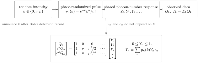
Decoy-state estimation is a constrained linear inverse problem. Vacuum, weak-decoy, and signal settings probe the same yields $Y_n$ with different known Poisson weights. Error gains obey an analogous system with unknowns $Y_ne_n$.

Yields, Gains, and Error Gains

Suppress the basis label temporarily. For an emitted $n$-photon pulse, define the yield

$$Y_n := \Pr(\text{Bob records an accepted detection}\mid n).$$

Define the conditional error rate

$$e_n := \Pr(\text{wrong bit}\mid n,\text{ accepted detection}).$$

For intensity $k$, the experimentally accessible gain and error gain are

$$Q_k := \Pr(\text{accepted detection}\mid k), \qquad T_k := E_kQ_k,$$

where $E_k$ is the observed QBER among detected rounds of that intensity. The Poisson mixture and conditional-indistinguishability assumption give

$$Q_k = \sum_{n=0}^{\infty}p_n(k)Y_n, \qquad T_k = \sum_{n=0}^{\infty}p_n(k)Y_ne_n.$$

It is useful to remove the common Poisson factor:

$$S_k:=e^kQ_k = \sum_{n=0}^{\infty}\frac{k^n}{n!}Y_n,$$ $$R_k:=e^kT_k = \sum_{n=0}^{\infty}\frac{k^n}{n!}Y_ne_n.$$

These are exponential generating functions for the yields and error yields. With an ideal continuum of exactly known intensities near zero,

$$Y_n = \left.\frac{d^nS_k}{dk^n}\right|_{k=0}, \qquad Y_ne_n = \left.\frac{d^nR_k}{dk^n}\right|_{k=0}.$$

This infinite-decoy limit gives the clean intuition. A practical experiment uses only a few intensities and finite counts, so it obtains bounds rather than an exact inversion.

The same definitions are applied separately by basis in a modern proof. For example, $Y_{n,Z}$ and the number of detected single-photon $Z$-basis signals enter the key length, while $X$-basis data help bound the corresponding phase error. Writing one basis-independent $Y_n$ is an expository simplification, not permission to average incompatible data sets.

Vacuum-Plus-Weak Bounds

The three settings $0<\nu<\mu$ already give a useful analytic estimate. For a true vacuum decoy,

$$Y_0=Q_0.$$

Background detections are often modeled as random bits, giving $e_0=1/2$. That value is a model choice to be checked against the receiver and its assignment rules; the vacuum data themselves estimate the background yield.

Lower bound on the one-photon yield

Expand the weak and signal gains:

$$S_\nu = Y_0+\nu Y_1 +\sum_{n=2}^{\infty}\frac{\nu^n}{n!}Y_n,$$ $$S_\mu = Y_0+\mu Y_1 +\sum_{n=2}^{\infty}\frac{\mu^n}{n!}Y_n.$$

Form the combination

$$\begin{aligned} D &:=S_\nu-\frac{\nu^2}{\mu^2}S_\mu \\ &= \left(1-\frac{\nu^2}{\mu^2}\right)Y_0 +\nu\left(1-\frac{\nu}{\mu}\right)Y_1 \\ &\quad+ \sum_{n=2}^{\infty} \frac{\nu^2}{n!} \left(\nu^{n-2}-\mu^{n-2}\right)Y_n. \end{aligned}$$

Because $0<\nu<\mu$ and $Y_n\ge0$, every term in the last line is nonpositive. The $n=2$ coefficient vanishes, and the coefficients for $n>2$ are negative. Therefore

$$D \le \left(1-\frac{\nu^2}{\mu^2}\right)Y_0 +\nu\left(1-\frac{\nu}{\mu}\right)Y_1.$$

Solving for $Y_1$ gives the standard vacuum-plus-weak lower bound

$$Y_1^{\mathrm L} = \frac{\mu}{\mu\nu-\nu^2} \left[ Q_\nu e^\nu -\frac{\nu^2}{\mu^2}Q_\mu e^\mu -\frac{\mu^2-\nu^2}{\mu^2}Y_0 \right].$$

An implementation clips an analytic estimate to the physical interval $0\le Y_1\le1$. In finite data, confidence bounds must be inserted with the directions that make $Y_1^{\mathrm L}$ smallest: a lower bound for $Q_\nu$ and upper bounds for $Q_\mu$ and $Y_0$ in this expression. A composable proof should derive those substitutions within its chosen statistical framework rather than treat point estimates as exact probabilities.

The single-photon contribution to signal-intensity detections is then bounded by

$$Q_1^{\mathrm L} = p_1(\mu)Y_1^{\mathrm L} = \mu e^{-\mu}Y_1^{\mathrm L}.$$

Upper bound on the one-photon error rate

All error-yield terms are nonnegative, so the weak-decoy error gain satisfies

$$R_\nu = e_0Y_0+\nu e_1Y_1 +\sum_{n=2}^{\infty} \frac{\nu^n}{n!}Y_ne_n \ge e_0Y_0+\nu e_1Y_1.$$

Consequently,

$$e_1^{\mathrm U} = \frac{E_\nu Q_\nu e^\nu-e_0Y_0} {\nu Y_1^{\mathrm L}}.$$

The numerator is made large and the denominator small when converting this formula into a finite-statistics bound. Physical clipping, zero denominators, and an apparently negative background-subtracted numerator need explicit handling. Many proofs cap a bit-error estimate at $1/2$ because larger values are no more useful for binary privacy amplification, but the permitted cap and its meaning belong to the proof being implemented.

These compact formulas are not the only decoy estimator. Linear or convex programs can incorporate more intensities, calibration intervals, basis dependence, and finite-count constraints without forcing each uncertainty through a hand-derived expression.

Worked Channel Example

Take an illustrative threshold-detector model with overall one-photon transmission-and-detection efficiency $\eta$, background yield $Y_0$, background error probability $e_0=1/2$, and optical misalignment error $e_d$. A simple low-background model is

$$Q_k = 1-(1-Y_0)e^{-\eta k},$$ $$T_k \simeq e_0Y_0+e_d\left(1-e^{-\eta k}\right).$$

The second expression neglects the small overlap between a background event and a signal-origin event; it is a calculation model, not a detector security proof. Choose

$$\mu=0.5, \qquad \nu=0.1, \qquad \eta=0.02, \qquad Y_0=10^{-6}, \qquad e_d=0.015.$$

The predicted signal and decoy observations are

$$\begin{aligned} Q_\mu&=9.95116\times10^{-3}, &E_\mu&=1.50488\times10^{-2},\\ Q_\nu&=1.99900\times10^{-3}, &E_\nu&=1.52426\times10^{-2}. \end{aligned}$$

Substitution in the analytic bounds gives

$$Y_1^{\mathrm L}=1.94001\times10^{-2}, \qquad e_1^{\mathrm U}=1.71002\times10^{-2},$$

and hence

$$Q_1^{\mathrm L} = \mu e^{-\mu}Y_1^{\mathrm L} = 5.88338\times10^{-3}.$$

For comparison, the channel model’s actual one-photon yield is

$$Y_1 = 1-(1-Y_0)(1-\eta) = 2.00010\times10^{-2}.$$

The bound is lower, as it must be, but remains close enough to certify a substantial single-photon contribution. Without intensity variation, the same overall signal gain would not determine that contribution.

From a Yield Bound to a Key Rate

In the asymptotic tagged-signal picture, multiphoton signal detections are treated as fully compromised and only single-photon detections contribute privacy. A widely used BB84 ledger is

$$R \ge q\left[ -Q_\mu f_{\mathrm{EC}}h_2(E_\mu) +Q_1^{\mathrm L} \left(1-h_2(e_1^{\mathrm U})\right) \right],$$

where

$$h_2(x) = -x\log_2x-(1-x)\log_2(1-x)$$

is the binary entropy, $f_{\mathrm{EC}}\ge1$ describes reconciliation inefficiency, and $q$ is a declared signal-and-basis selection prefactor. In the traditional symmetric BB84 convention with an asymptotically negligible decoy fraction, $q=1/2$. If signal intensity is chosen with probability $p_\mu$ and only $Z$-$Z$ rounds make key, then a per-emitted-pulse ledger instead contains the corresponding factor $q=p_\mu p_Z^{A}p_Z^{B}$.

For the numerical example, taking $f_{\mathrm{EC}}=1.16$ gives the bracketed quantity

$$-Q_\mu f_{\mathrm{EC}}h_2(E_\mu) +Q_1^{\mathrm L} \left(1-h_2(e_1^{\mathrm U})\right) = 3.84852\times10^{-3}.$$

Thus the conventional $q=1/2$ example yields approximately $1.92\times10^{-3}$ secret bits per emitted pulse before finite-key, authentication, and other implementation overheads. A positive asymptotic number is not a claim about a finite device run.

The formula also hides an important proof step. In BB84, privacy amplification depends on a single-photon phase-error rate. Under the symmetry and source assumptions of the relevant proof, conjugate-basis single-photon observations bound that phase error. One must not insert an arbitrary aggregate optical QBER into the privacy term merely because it has a similar numerical value.

Finite-Key Estimation

A real block supplies counts, not exact probabilities. For each intensity and basis class, let

$$N_{k,b}=\text{number sent}, \qquad n_{k,b}=\text{accepted detections}, \qquad m_{k,b}=\text{wrong detected bits}.$$

The observed ratios are

$$\widehat Q_{k,b} = \frac{n_{k,b}}{N_{k,b}}, \qquad \widehat T_{k,b} = \frac{m_{k,b}}{N_{k,b}}.$$

Composable finite-key analysis replaces these ratios by simultaneous confidence bounds whose failure probabilities are included in the total security budget. One convenient abstract form is

$$\underline Q_{k,b} \le \sum_{n=0}^{\infty}p_n(k)Y_{n,b} \le \overline Q_{k,b},$$ $$\underline T_{k,b} \le \sum_{n=0}^{\infty}p_n(k)Y_{n,b}e_{n,b} \le \overline T_{k,b}.$$

Subject to $0\le Y_{n,b}\le1$ and $0\le Y_{n,b}e_{n,b}\le Y_{n,b}$, Alice and Bob minimize the desired single-photon count and maximize the relevant error parameter. A numerical linear program truncates the photon number at $n_{\max}$ and accounts for the known Poisson tail

$$\tau_k(n_{\max}) = 1- \sum_{n=0}^{n_{\max}}e^{-k}\frac{k^n}{n!}.$$

The tail cannot simply be discarded; it must be assigned in the adverse direction allowed by the constraints.

A typical finite-key result has the structure

$$\ell \le s_{Z,1}^{\mathrm L} \left[1-h_2(\phi_Z^{\mathrm U})\right] -\lambda_{\mathrm{EC}} -\Delta_{\mathrm{sec}},$$

where $s_{Z,1}^{\mathrm L}$ bounds detected one-photon key-basis events, $\phi_Z^{\mathrm U}$ bounds their phase-error rate, $\lambda_{\mathrm{EC}}$ is the actual reconciliation leakage, and $\Delta_{\mathrm{sec}}$ collects verification, smoothing, privacy amplification, and declared failure-probability terms. The exact coefficients depend on the proof. The finite-key analysis of Lim et al. is one important composable construction against general attacks; one-decoy analyses require their own bounds and allocation choices.

Why more decoys can still mean less key

Additional intensity settings add constraints, but finite samples must be divided among more classes. A very weak decoy is informative about $Y_1$ only if it produces enough detections to control fluctuations. A vacuum setting measures background directly but produces few useful events by design. The signal intensity, decoy intensities, basis biases, and selection probabilities therefore need joint optimization for the expected channel, block duration, detector behavior, and security target.

Rules of thumb such as $\mu\approx0.5$ and $\nu\approx0.1$ are useful starting points for some fiber links, not protocol constants. At long distance, the best allocation may devote a substantial fraction of pulses to parameter estimation. In a changing channel, an optimization based on a favorable past block can also bias the analysis unless adaptation is specified in advance or covered by the proof.

Source Assumptions That Carry the Proof

Phase randomization

The Poisson mixture follows from averaging a uniformly random global phase. Attenuation alone does not perform that average. Gain-switching a laser may produce substantial phase randomization under characterized operating conditions, but it is not a mathematical guarantee for every pulse. Residual phase coherence can let Eve distinguish or coherently combine states in ways excluded by the photon-number-channel model. A transmitter should actively randomize or otherwise validate the phase model used by its proof.

Protocols with nonrandom or partially known phase can still have security proofs, but the proof and state decomposition are different. The standard decoy equations must not be imported unchanged.

Intensity calibration and fluctuations

The symbols $\mu$ and $\nu$ represent physical photon-number distributions, not merely digital control values. Modulator calibration, laser power drift, finite extinction, pulse-shape changes, and monitor uncertainty produce intervals or correlations in the actual intensities. A sound analysis either bounds the emitted distribution pulse by pulse or uses a security proof that explicitly tolerates the characterized fluctuation model.

Replacing an uncertain $k$ by its nominal value can move Poisson weights in the favorable direction and overestimate $Y_1$. The conservative endpoint is not always the same for every coefficient, so blindly inserting one worst intensity into every term is not generally valid.

No intensity side channel at fixed photon number

Signal and decoy pulses can differ in spectrum, timing, chirp, spatial mode, polarization, pulse duration, or back-reflected light. If Eve can infer the intensity class before acting on the pulse, the correct variables are $Y_{n,k}$ rather than shared $Y_n$. The standard system then loses its cross-intensity constraint.

This issue is especially important when separate lasers generate signal and decoy pulses. A single laser followed by a characterized intensity modulator can reduce some differences, but the modulator itself can introduce chirp or pattern dependence. Optical isolation, filtering, watchdog monitoring, and Trojan-horse bounds address parts of the engineering problem; their residual assumptions still belong in the security statement.

Correlations and detector behavior

Dead time, afterpulsing, modulator memory, feedback control, and thermal drift can correlate neighboring rounds. A proof based on independent and identically distributed trials is not automatically valid for such a source or receiver. Modern analyses may use martingale, entropy-accumulation, or explicit source-memory methods, but the observed data must match the chosen model.

Decoy states do not remove detector side channels. Detector blinding, efficiency mismatch, time-shift attacks, and mode-dependent acceptance remain receiver-model questions. Measurement-Device-Independent QKD combines two-source decoy estimation with an untrusted measurement station to move that particular trust boundary; it still relies on source characterization and decoy-state assumptions.

Protocol Variants

Vacuum plus weak decoy

The signal, weak-decoy, and vacuum settings used above are often called a two-decoy protocol because there are two nonsignal intensities. It gives simple analytic bounds and can approach the asymptotic performance of an ideal many-decoy protocol under the standard source model.

One-decoy protocols

A signal plus one nonzero decoy removes the dedicated vacuum setting. The background yield must then be bounded indirectly or through other data. This can simplify high-speed hardware and improve finite allocation in some regimes, but it changes the estimator. A vacuum-plus-weak formula with an unmeasured $Y_0$ must not be presented as a one-decoy result.

Biased-basis and four-intensity designs

Efficient BB84 strongly favors the key basis and reserves the conjugate basis for phase-error estimation. Some practical protocols choose intensities with basis-dependent probabilities or use a dedicated intensity in each basis. The resulting rate can improve, but basis and intensity labels must remain in the parameter-estimation bookkeeping. Pooling all gains into one basis-free table may erase exactly the distinction the security proof needs.

Passive decoys and heralded sources

Instead of actively modulating each pulse, a transmitter can infer intensity classes from a correlated local measurement or passive optical network. Heralded parametric sources lead to related photon-number conditioning. These schemes can reduce active modulation leakage, but the conditional source states and monitor detector must be modeled explicitly; they are not automatically equivalent to Poissonian active decoys.

What Decoy States Do Not Establish

Claim	What decoy analysis actually provides	What remains
“The source is now a single-photon source.”	A bound on detections attributable to the one-photon sector.	Vacuum and multiphoton pulses are still emitted.
“Photon-number splitting is impossible.”	A rate that remains secure while multiphoton rounds may be tagged.	The proof still needs valid source indistinguishability and statistics.
“A low QBER proves secrecy.”	Error gains help bound one-photon errors.	Phase errors, finite-size terms, leakage, and authentication remain.
“Detector attacks are closed.”	Nothing about an unmodeled receiver follows from changing source intensity.	Detector characterization, hardening, or a different trust architecture is required.
“Nominal intensities are enough.”	Known Poisson weights make the inverse problem possible.	Calibration uncertainty, drift, correlations, and side channels must be bounded.
“An asymptotic positive rate means this run made a key.”	The formula diagnoses an ideal large-block regime.	The actual transcript needs a finite-key proof and positive final length.

Common Mistakes

Treating $Q_\mu$ as the one-photon gain

$Q_\mu$ includes vacuum-background, one-photon, and multiphoton detections. The quantity entering the untagged privacy term is $Q_1=\mu e^{-\mu}Y_1$, bounded through all intensity classes.

Forgetting the exponential factor

The linear generating function is $S_k=e^kQ_k$, not $Q_k$. Omitting $e^k$ changes every coefficient and invalidates the analytic bound.

Reversing the inequality in the $Y_1$ derivation

For $n>2$, $\nu^{n-2}-\mu^{n-2}<0$. The discarded tail makes $D$ smaller, so the resulting inequality is an upper bound on $D$ and therefore a lower bound on $Y_1$.

Using point estimates in a finite run

$n_{k,b}/N_{k,b}$ fluctuates. Substituting it directly for $Q_{k,b}$ silently claims an infinite sample. Confidence failures must be allocated and composed with the other security errors.

Assuming the intensity label is the only difference

That is the hypothesis to validate, not a consequence of naming a pulse “decoy.” At fixed photon number, any exploitable spectral, temporal, spatial, or polarization difference can make the shared-yield equations false.

Exercises

1. Phase averaging

Starting from the coherent-state expansion, prove that uniform phase randomization produces a diagonal Poisson mixture.

Solution

Expand the projector:

$$|\alpha\rangle\langle\alpha| = e^{-k} \sum_{n,m=0}^{\infty} \frac{k^{(n+m)/2}e^{i(n-m)\phi}} {\sqrt{n!m!}}|n\rangle\langle m|.$$

Uniform averaging uses

$$\int_0^{2\pi}\frac{d\phi}{2\pi} e^{i(n-m)\phi} = \delta_{nm}.$$

Only $n=m$ remains, giving

$$\rho_k = \sum_{n=0}^{\infty} e^{-k}\frac{k^n}{n!}|n\rangle\langle n|.$$

2. Multiphoton probability

Show that $p_{\ge2}(k)=1-e^{-k}(1+k)$. Find its leading behavior for $k\ll1$ and evaluate it at $k=0.5$.

Solution

Subtract the vacuum and one-photon probabilities from unity:

$$p_{\ge2}(k) = 1-p_0(k)-p_1(k) = 1-e^{-k}(1+k).$$

Using $e^{-k}=1-k+k^2/2+O(k^3)$ gives

$$p_{\ge2}(k) = \frac{k^2}{2}+O(k^3).$$

At $k=0.5$,

$$p_{\ge2}(0.5) = 1-1.5e^{-0.5} \approx 0.0902.$$

Thus roughly nine percent of emitted signal pulses are multiphoton in this source model, even though loss makes the detected fraction quite different.

3. Derive the one-photon yield bound

For $0<\nu<\mu$, derive the vacuum-plus-weak lower bound on $Y_1$ by forming $S_\nu-(\nu^2/\mu^2)S_\mu$. State where nonnegativity is used.

Solution

The combination is

$$\begin{aligned} S_\nu-\frac{\nu^2}{\mu^2}S_\mu &= \left(1-\frac{\nu^2}{\mu^2}\right)Y_0 +\nu\left(1-\frac{\nu}{\mu}\right)Y_1\\ &\quad+ \sum_{n=2}^{\infty} \frac{\nu^2}{n!} \left(\nu^{n-2}-\mu^{n-2}\right)Y_n. \end{aligned}$$

The tail is nonpositive because $Y_n\ge0$ and $\nu^{n-2}-\mu^{n-2}\le0$. Dropping it therefore increases the right-hand side. Rearranging the resulting inequality and inserting $S_k=e^kQ_k$ gives

$$Y_1 \ge \frac{\mu}{\mu\nu-\nu^2} \left[ Q_\nu e^\nu -\frac{\nu^2}{\mu^2}Q_\mu e^\mu -\frac{\mu^2-\nu^2}{\mu^2}Y_0 \right].$$

4. Derive the error bound

Starting from $R_\nu$, derive an upper bound on $e_1$. Explain why replacing $Y_1$ by a lower bound is conservative.

Solution

Nonnegative multiphoton error yields imply

$$R_\nu \ge e_0Y_0+\nu e_1Y_1.$$

Therefore

$$e_1 \le \frac{R_\nu-e_0Y_0}{\nu Y_1} = \frac{E_\nu Q_\nu e^\nu-e_0Y_0}{\nu Y_1}.$$

For a nonnegative numerator, decreasing the denominator increases the ratio. Using $Y_1^{\mathrm L}\le Y_1$ therefore preserves an upper bound. A finite analysis separately bounds each observed quantity and handles an unfavorable or statistically negative background-subtracted numerator according to its optimization procedure.

5. Reproduce the channel estimate

Use the worked-example parameters to calculate $Y_1^{\mathrm L}$, $e_1^{\mathrm U}$, and $Q_1^{\mathrm L}$. Compare the yield bound with the model value $1-(1-Y_0)(1-\eta)$.

Solution

The gains and error rates are

$$\begin{aligned} Q_{0.5}&=0.0099511563, &E_{0.5}&=0.0150487531,\\ Q_{0.1}&=0.0019989993, &E_{0.1}&=0.0152426364. \end{aligned}$$

Substitution gives

$$Y_1^{\mathrm L}=0.0194001076, \qquad e_1^{\mathrm U}=0.0171002041,$$

and

$$Q_1^{\mathrm L} = 0.5e^{-0.5}Y_1^{\mathrm L} = 0.0058833800.$$

The model value is $Y_1=0.02000098$, so the analytic lower bound is about $97.0\%$ of the actual value in this noiseless, asymptotic calculation.

6. Infinite-decoy reconstruction

Suppose $Q_k$ is known exactly for all $k$ in a neighborhood of zero. Show how to reconstruct $Y_0$, $Y_1$, and $Y_2$.

Solution

Define $S_k=e^kQ_k$. Its series is

$$S_k = Y_0+kY_1+\frac{k^2}{2}Y_2+\cdots.$$

Hence

$$Y_0=S_0, \qquad Y_1=S'_0, \qquad Y_2=S''_0.$$

In general $Y_n=S^{(n)}_0$. Exact differentiation is only an intuition for the infinite-data, continuous-intensity limit; numerical differentiation of noisy experimental gains would be unstable.

7. A distinguishable-decoy failure

Suppose weak-decoy pulses are delayed by $200\ \mathrm{ps}$ relative to signal pulses, and Eve can resolve that delay before deciding whether to forward a pulse. Identify the failed equation and explain what extra evidence or analysis is needed.

Solution

At fixed photon number, Eve can infer the class from arrival time. The shared yield model fails: one must allow

$$Y_{n,\nu}\ne Y_{n,\mu}, \qquad e_{n,\nu}\ne e_{n,\mu}.$$

Then comparing $Q_\nu$ and $Q_\mu$ no longer constrains one common $Y_1$. Alice needs source characterization showing that the delay is absent or bounded strongly enough for a proof with distinguishable states, or she needs a protocol and security analysis that explicitly includes the leaked timing information. Relabeling the pulses does not repair the model.

8. Finite-key resource allocation

Alice can reduce the weak-decoy probability to send more signal pulses. Give one benefit and two costs of doing so in a fixed-duration experiment.

Solution

The benefit is a larger expected number of signal-and-key-basis detections, which can increase the raw material for the final key. The costs are fewer weak-decoy detections and therefore wider confidence intervals for $Y_1$ and $e_1$. A looser lower bound on $s_{Z,1}$ or a looser upper bound on the phase error can erase the gain or force abort. The best probability is therefore a finite-block optimization, not “as few decoys as possible.” Channel drift can add a third cost if the smaller sample no longer diagnoses nonstationarity.

Further Connections

• Quantum Key Distribution supplies the composable secrecy, authentication, distillation, and finite-key contract around this estimator.
• BB84 develops the four-state transcript and the single-photon bit–phase error relation used by the privacy term.
• Measurement-Device-Independent QKD generalizes the gain equations to photon-number pairs $Y_{nm}$ and moves all relay detectors outside the trusted boundary.
• Photon-Number States develops Fock states, number statistics, and optical detection language.
• Coherent States derives coherent-state amplitudes and their Poisson number distribution.
• Photonic Qubits owns source, encoding, loss, mode, and detector hardware considerations.
• Cryptography Case Studies applies decoy estimation inside a concrete lossy-fiber rate and distance ledger.
• Trace Distance explains the operational metric behind composable secrecy.

References

1. W.-Y. Hwang, “Quantum Key Distribution with High Loss: Toward Global Secure Communication,” Physical Review Letters 91, 057901 (2003), doi:10.1103/PhysRevLett.91.057901.
2. H.-K. Lo, X. Ma, and K. Chen, “Decoy State Quantum Key Distribution,” Physical Review Letters 94, 230504 (2005), doi:10.1103/PhysRevLett.94.230504.
3. X.-B. Wang, “Beating the Photon-Number-Splitting Attack in Practical Quantum Cryptography,” Physical Review Letters 94, 230503 (2005), doi:10.1103/PhysRevLett.94.230503.
4. X. Ma, B. Qi, Y. Zhao, and H.-K. Lo, “Practical Decoy State for Quantum Key Distribution,” Physical Review A 72, 012326 (2005), doi:10.1103/PhysRevA.72.012326.
5. D. Gottesman, H.-K. Lo, N. Lütkenhaus, and J. Preskill, “Security of Quantum Key Distribution with Imperfect Devices,” Quantum Information and Computation 4, 325–360 (2004), doi:10.26421/QIC4.5-1.
6. H.-K. Lo and J. Preskill, “Security of Quantum Key Distribution Using Weak Coherent States with Nonrandom Phases,” Quantum Information and Computation 7, 431–458 (2007), doi:10.26421/QIC7.5-6-2.
7. C. C. W. Lim, M. Curty, N. Walenta, F. Xu, and H. Zbinden, “Concise Security Bounds for Practical Decoy-State Quantum Key Distribution,” Physical Review A 89, 022307 (2014), doi:10.1103/PhysRevA.89.022307.
8. D. Rusca, A. Boaron, F. Grünenfelder, A. Martin, and H. Zbinden, “Finite-Key Analysis for the 1-Decoy State QKD Protocol,” Applied Physics Letters 112, 171104 (2018), doi:10.1063/1.5023340.
9. V. Scarani, H. Bechmann-Pasquinucci, N. J. Cerf, et al., “The Security of Practical Quantum Key Distribution,” Reviews of Modern Physics 81, 1301–1350 (2009), doi:10.1103/RevModPhys.81.1301.
10. F. Xu, X. Ma, Q. Zhang, H.-K. Lo, and J.-W. Pan, “Secure Quantum Key Distribution with Realistic Devices,” Reviews of Modern Physics 92, 025002 (2020), doi:10.1103/RevModPhys.92.025002.
11. D. Rosenberg, J. W. Harrington, P. R. Rice, et al., “Long-Distance Decoy-State Quantum Key Distribution in Optical Fiber,” Physical Review Letters 98, 010503 (2007), doi:10.1103/PhysRevLett.98.010503.
12. T. Schmitt-Manderbach, H. Weier, M. Fürst, et al., “Experimental Demonstration of Free-Space Decoy-State Quantum Key Distribution over 144 km,” Physical Review Letters 98, 010504 (2007), doi:10.1103/PhysRevLett.98.010504.
13. C.-Z. Peng, J. Zhang, D. Yang, et al., “Experimental Long-Distance Decoy-State Quantum Key Distribution Based on Polarization Encoding,” Physical Review Letters 98, 010505 (2007), doi:10.1103/PhysRevLett.98.010505.
14. A. Boaron, G. Boso, D. Rusca, et al., “Secure Quantum Key Distribution over 421 km of Optical Fiber,” Physical Review Letters 121, 190502 (2018), doi:10.1103/PhysRevLett.121.190502.
15. K. Tamaki, M. Curty, G. Kato, H.-K. Lo, and K. Azuma, “Loss-Tolerant Quantum Cryptography with Imperfect Sources,” Physical Review A 90, 052314 (2014), doi:10.1103/PhysRevA.90.052314.

Summary

Phase randomization turns a weak coherent pulse of mean photon number $k$ into the Poisson mixture

$$\rho_k = \sum_{n=0}^{\infty}e^{-k}\frac{k^n}{n!}|n\rangle\langle n|.$$

Random signal and decoy intensities apply different known weights to the same conditional yields $Y_n$ and error yields $Y_ne_n$. Their measured gains therefore bound the one-photon signal contribution even when Eve controls the lossy channel. Vacuum-plus-weak data give analytic bounds on $Y_1$ and $e_1$; finite protocols replace exact gains by confidence regions and convert the result into a bound on single-photon key events and phase errors.

The method is only as trustworthy as its source model. Phase randomization, intensity calibration, fixed-$n$ indistinguishability, side-channel control, correlation treatment, detector assumptions, and the complete composable postprocessing ledger all remain part of the security claim.