Quantum Repeaters

A quantum repeater distributes usable quantum correlations across a long, lossy, or noisy path by dividing it into shorter elementary links and joining their quantum resources at intermediate nodes. Depending on the architecture, the node stores heralded entanglement, performs entanglement swapping and distillation, applies quantum error correction, or prepares a photonic graph state whose measurements accomplish the same logical task.

The word repeater does not mean that an unknown qubit is measured, copied, and regenerated. No-Cloning and No-Signaling forbids that classical strategy. Nor is every middle station a repeater. A trusted key relay, optical amplifier, measurement-device-independent QKD relay, postselected swap, and satellite downlink have different resources and trust models.

This page is the canonical home for repeater architecture: the loss problem, elementary-link contract, stochastic synchronization, memory-age policy, nested connection, error-control choices, repeater generations, all-photonic designs, scheduling, resource ledgers, and criteria for an end-to-end repeater claim. Entanglement Swapping owns the Bell-basis identity and Pauli-frame update. Entanglement Distillation owns purification maps and yields. Quantum Memories owns write–store–read hardware. Network Case Studies owns detailed experimental comparisons and complete evidence ledgers.

Why Direct Transmission Fails at Long Distance

For a fiber with attenuation coefficient $\alpha$ in decibels per unit length, the channel transmissivity is

$$\eta(L) = 10^{-\alpha L/10}.$$

At $\alpha=0.2\ \mathrm{dB/km}$, every additional $50\ \mathrm{km}$ costs a factor of ten in transmission probability. Faster sources improve the number of attempts per second, but they do not change this exponential dependence on $L$.

For an ideal pure-loss bosonic channel, the ultimate two-way-assisted secret-key and entanglement-distribution rate per optical mode is the repeaterless value

$$K_{\mathrm{PLOB}}(\eta) = -\log_2(1-\eta) \simeq \frac{\eta}{\ln 2}$$

at high loss. A practical direct apparatus can operate far below this bound. Beating that apparatus is useful engineering progress; beating the bound under matched modes, channel uses, directions, and trust assumptions is a stronger claim.

Segmentation alone changes nothing

Suppose a path is divided into $m$ independent segments and all segments must succeed in the same clock cycle because no quantum state can wait. If segment $j$ succeeds with probability $p_j$, then

$$p_{\mathrm{sim}} = \prod_{j=1}^{m}p_j.$$

For ideal transmission factors with $\prod_j\eta_j=\eta(L)$, the product has the same exponential loss as the original path, with additional interface and detector penalties. Shorter spans become useful only when the protocol can retain or encode progress rather than demanding simultaneous end-to-end survival.

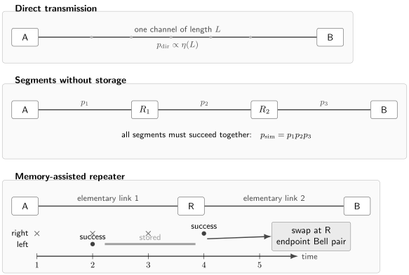
Why storage changes the stochastic problem. A direct photon must survive the full length. Memoryless segmentation still multiplies simultaneous segment successes. A memory-assisted repeater can keep the left link from cycle 2 while the right link succeeds in cycle 4, then swap at the middle node. The gain is purchased with memory time, local operations, heralding, classical control, and extra physical resources.

The Repeater Service Contract

The output should be named before the architecture is optimized. A common request is one Bell pair between endpoint registers $A$ and $B$ with fidelity at least $F_{\min}$. Other services request a secret key, teleported qubit, remote logical gate, graph-state edge, or distributed sensor state.

A Bell-pair service can be summarized by

$$\mathcal S_{AB} = \left( \rho_{\mathrm{tar}}, F_{\min}, R_{\mathrm{del}}, P_{\mathrm{lat}}, \varepsilon_{\mathrm{false}}, A_{\mathrm{svc}}, \mathcal T \right).$$

Here $R_{\mathrm{del}}$ is the rate after all retries, swaps, error control, cutoffs, and readout losses; $P_{\mathrm{lat}}$ is the latency distribution; $\varepsilon_{\mathrm{false}}$ bounds false heralds or wrong accepted output; $A_{\mathrm{svc}}$ is availability; and $\mathcal T$ states the trust model. The pair is delivered only when it occupies the advertised endpoint registers and is ready for the next advertised operation.

At least three event denominators should remain visible:

1. optical modes or elementary attempts launched;
2. local heralds and swaps accepted;
3. endpoint states delivered above the service threshold.

Conditional fidelity uses the second or third denominator. Throughput uses the first. A high-fidelity pair reconstructed after severe postselection is not automatically a high-rate service.

Elementary-Link Generation

An elementary link joins neighboring nodes separated by $L_0$. Many protocols place an optical Bell analyzer near the midpoint, so photons travel about $L_0/2$ from each node. A schematic two-photon heralding probability is

$$\begin{aligned} p_0 \approx{}& p_{\mathrm{emit}}^2 \eta_{\mathrm{int}}^2 \eta_{\mathrm f}(L_0/2)^2\\ &\times \eta_{\mathrm{det}}^2 p_{\mathrm{BSM}}. \end{aligned}$$

$p_{\mathrm{emit}}$ includes successful spin–photon or memory–photon state generation, $\eta_{\mathrm{int}}$ includes collection and conversion, $\eta_{\mathrm f}$ is fiber transmission, $\eta_{\mathrm{det}}$ is detector efficiency, and $p_{\mathrm{BSM}}$ is the accepted Bell-measurement fraction. The expression is not universal. Single-photon protocols, direct absorption, satellite links, cavity gates, and multiplexed schemes have different powers and correlated failure terms.

The attempt period cannot be inferred from a source clock alone. If the node must wait for a remote success or failure message before reusing a memory,

$$\tau_0 \gtrsim \tau_{\mathrm{prepare}} + \tau_{\mathrm{optical}} + \tau_{\mathrm{herald}} + \tau_{\mathrm{reset}}.$$

Depending on where detection and control decisions occur, $\tau_{\mathrm{herald}}$ contains one-way or round-trip propagation over part of $L_0$. A quoted megahertz emitter does not imply a megahertz independent link-attempt rate if only one memory mode is available.

Heralding must be trustworthy

A useful elementary event is heralded online and leaves a quantum state available at both nodes. Dark counts, multiphoton emission, double excitation, mode mismatch, and readout errors create false heralds. The link contract must report both

$$p_0 \quad\text{and}\quad \rho_0\mid\mathrm{herald},$$

not one without the other. Background subtraction may diagnose hardware, but raw false-herald probability determines how the repeater behaves.

Synchronizing Probabilistic Links

Let each of two links be attempted once per interval and succeed independently with probability $p$. The waiting times $N_1,N_2\in\{1,2,\ldots\}$ are geometric:

$$\Pr(N_i=n) = (1-p)^{n-1}p.$$

Both links are ready after $N_{\max}=\max(N_1,N_2)$ intervals. Its exact mean is

$$\mathbb E[N_{\max}] = \frac{3-2p}{p(2-p)} \simeq \frac{3}{2p}$$

for $p\ll1$. The earlier pair waits, on average,

$$\mathbb E[|N_1-N_2|] = \frac{2(1-p)}{p(2-p)} \simeq \frac1p$$

additional intervals. Thus a memory must usually survive much longer than one attempt. For $m$ equal links prepared in parallel, the small-$p$ behavior is

$$\mathbb E[N_{\max}] \simeq \frac{H_m}{p}, \qquad H_m = \sum_{j=1}^{m}\frac1j.$$

The logarithmic growth of $H_m$ is far better than demanding simultaneous success with probability $p^m$, but only if enough memories, modes, and local switching exist to keep the successes.

Memory age and cutoff policy

Memory quality is a function of age. A useful phenomenological ledger is

$$v(t) = \exp\left[-\left(\frac{t}{T_2}\right)^\beta\right], \qquad \eta_{\mathrm m}(t),$$

where $v(t)$ tracks coherence visibility and $\eta_{\mathrm m}(t)$ tracks retrieval. Conditioning only on successful retrieval can hide a low unconditional rate.

A scheduler may discard an old link after $k_c$ additional attempts. Given that one link has just succeeded, the probability that an independent partner arrives within the next $k_c$ trials is

$$P_{\mathrm{match}}(k_c) = 1-(1-p)^{k_c}.$$

Larger $k_c$ wastes fewer early successes but admits older, noisier states. The optimum depends on the fidelity threshold, latency objective, swap policy, and memory channel. There is no universally optimal timeout.

Multiplexing

If $M$ independent modes are genuinely available in one cycle, the probability of at least one success is

$$p_M = 1-(1-p)^M \simeq Mp$$

for $Mp\ll1$. Temporal, spectral, spatial, frequency-bin, and multi-emitter multiplexing can reduce waiting. Nominal mode count is not effective mode count unless successful modes can be identified, stored, routed, matched, and read independently without saturating shared detectors or control hardware.

Swapping and Nested Connection

Once adjacent links are ready, an intermediate node performs a Bell measurement or equivalent local operation. This consumes the two short pairs and creates a longer endpoint pair, conditioned on the swap result. The result also determines a Pauli frame that must be communicated or tracked. The canonical state identity and noisy Bell-diagonal examples are derived in Entanglement Swapping.

For $2^k$ equal elementary links, a binary nested schedule has levels $\ell=0,1,\ldots,k$. Level 0 prepares length-$L_0$ pairs; level 1 joins pairs across $2L_0$; level 2 joins those across $4L_0$; and so on.

Under a deliberately simple rare-success model, let $T_\ell$ be the mean time to obtain one accepted level-$\ell$ pair, and let $q_\ell$ be the probability that the swap and quality check at the next level keep the pair. Then

$$T_{\ell+1} \approx \frac{3}{2q_\ell}T_\ell + \tau_{\ell}^{\mathrm{ctrl}}.$$

The factor $3/2$ is the two-link synchronization penalty at small success probability. If swaps are deterministic, controls are fast, and every level has the same quality, nesting gives

$$T_k \sim \frac{\tau_0}{p_0} \left(\frac32\right)^k = \frac{\tau_0}{p_0} n^{\log_2(3/2)}, \qquad n=2^k,$$

rather than a simultaneous-success cost proportional to $p_0^{-n}$. This polynomial-scaling illustration is not a universal repeater-rate law. Finite buffers, failed swaps, nonidentical links, age-dependent states, purification, classical latency, resource contention, and parallel requests change the recurrence.

Swap-as-soon-as-possible is not always optimal

Immediately swapping any ready neighboring links reduces memory age, but it can create mismatched link lengths, consume scarce memories, or produce a long pair that waits even longer for a partner. Other policies reserve pairs for balanced nesting levels, prioritize youngest or highest-fidelity states, or optimize a deadline-aware application utility. The best policy depends on the complete network state, not only on which edges are occupied.

Controlling Accumulated Errors

Range extension normally reduces quality. Memory dephasing, imperfect local gates, readout faults, leakage, phase-reference errors, and false heralds accumulate with every level. A repeater therefore needs an explicit quality strategy.

Entanglement distillation

First-generation designs consume several noisy pairs to probabilistically produce fewer better pairs. Purification may occur at elementary and nested levels. It requires two-way classical communication and additional waiting, and a failed round may destroy both inputs. Entanglement Distillation owns recurrence protocols, acceptance probabilities, hashing yield, local noise, and distillability limits.

Quantum error correction

Encoded repeaters protect a logical qubit or logical Bell pair against erasure and operational faults. Located photon loss is structurally different from an unflagged Pauli error, so code selection and decoder assumptions matter. A third-generation design must correct loss quickly enough for one-way operation and suppress local operation errors below a logical target.

The Threshold Theorem owns fault-tolerance conditions. A statement that a repeater uses error correction is incomplete without the code, erasure and gate error model, syndrome circuit, decoder latency, logical failure target, and physical overhead.

Repeater Generations and Architectures

The common three-generation classification asks how loss and operation errors are handled. It is a resource taxonomy, not a chronology or quality ranking.

Architecture	Loss handling	Operation-error handling	Long-distance signaling	Main advantage	Main burden
first generation	heralded elementary generation	heralded purification	two-way at multiple nesting levels	modest local processor size and tolerant of probabilistic links	long memories and latency-limited rate
second generation	heralded elementary generation	quantum error correction	two-way for link generation, mostly one-way afterward	removes repeated purification latency	many high-quality local qubits and gates
third generation	quantum error correction for loss	quantum error correction	one-way	high throughput in principle	stringent coupling, loss, gate, and code thresholds

Which generation minimizes resources depends on distance, attenuation, coupling and detection efficiency, gate error and duration, memory coherence, node spacing, multiplexing, and the required output. A slower first-generation system can be preferable when excellent memories exist but local gate counts must stay small. A third-generation system can dominate only after its much larger node satisfies the relevant thresholds.

All-photonic repeaters

All-photonic protocols replace long-lived matter memories with large photonic cluster states, loss-tolerant tree encodings, and adaptive measurements. Photonic branching provides multiple chances to complete an effective Bell measurement or indirect measurement before the flying resource is lost.

This does not make the repeater resource-free. The burden moves to near-deterministic or highly multiplexed graph-state generation, low-loss delay, fast feed-forward, switching, number-resolving or high-efficiency detection, and management of a large number of optical modes. Calling the design “memoryless” should not hide short optical delays and synchronization needed within a station.

Hybrid and encoded-photonic designs

Many proposals combine matter communication qubits, long-lived local memories, multimode ensemble storage, telecom photons, bosonic loss codes, and photonic cluster states. “Hybrid” identifies an interface strategy, not a security or performance level. Every conversion and transfer must appear in the end-to-end efficiency and noise ledger.

Node Requirements

A complete repeater station is more than a memory plus fiber.

Node function	Required evidence
photonic interface	emission or absorption probability, indistinguishability, bandwidth, frequency conversion, added noise
memory bank	write and read efficiency, age-dependent channel, mode capacity, random access, cross-talk, reset
local processing	Bell-measurement success, gate and measurement errors, leakage, duration, parallelism
optical switching	insertion loss, extinction, routing latency, mode compatibility
reference distribution	clock, phase, polarization, and frequency stability under deployed conditions
controller	herald processing, Pauli frames, cutoff and swap policy, queueing, fault recovery
security boundary	authenticated classical messages, node trust, isolation, tamper and side-channel model

A useful memory ratio is

$$\Lambda = \frac{T_{\mathrm{useful}}}{\tau_0},$$

the number of elementary attempts that fit within useful storage. Large $T_2$ alone is not enough: low write efficiency, slow reset, one memory mode, or destructive readout may still make $\Lambda$ operationally small.

Interconnects and Transduction owns complete accepted-input-to-usable-output interfaces. Modular Architectures owns local processor composition and distributed fault domains. Quantum Network Architectures owns multiuser service layers, entanglement routing and inventory, control planes, and administrative trust boundaries.

Simulation and Scheduling

Average-link formulas are useful for orientation but can erase the variables a scheduler acts on. An event-driven simulation should retain, for every live edge resource $e$,

$$\mathcal X_e = \left( \rho_e, t_e, m_e, f_e, h_e, c_e \right),$$

where $\rho_e$ is the state or error summary, $t_e$ its age, $m_e$ the memory slot and mode, $f_e$ its Pauli frame, $h_e$ pending herald information, and $c_e$ the controller state. Events include link attempts, herald arrivals, timeouts, swaps, purification, retrieval, decoder completion, resets, and application requests.

A reproducible model should state:

• random-number seeds and the number of simulated service requests;
• channel, detector, memory, gate, and controller distributions;
• whether links and errors are independent, correlated, or drifting;
• buffer capacity, routing, cutoff, swap, purification, and retry policies;
• warm-up, calibration, and downtime assumptions;
• confidence intervals for rate, fidelity, latency quantiles, and failure.

Optimizing only the mean delivered rate can create unacceptable tail latency or unfairness among users. Deadline success, qubit-seconds, optical-mode use, energy, and service availability may belong in the objective.

Direct Benchmarks and Trust Models

A repeater claim needs a comparator with the same requested service.

• Direct transmission: count every optical mode, source attempt, detector, and temporal or spectral channel.
• Repeaterless capacity: state the channel model and whether the PLOB or another bound applies.
• Trusted relays: deployed QKD keys may be decrypted or combined at trusted nodes; this is not end-to-end untrusted entanglement distribution.
• Twin-field and related QKD: an untrusted middle measurement can improve rate–loss scaling without providing stored endpoint entanglement or a general quantum channel.
• Satellite links: long free-space spans can reduce attenuation relative to fiber, but a trusted satellite or source is not automatically a repeater.

An entanglement-based repeater can, in principle, leave intermediate stations untrusted for an end-to-end cryptographic task because the endpoints test the delivered correlations. A compromised node can still deny service, bias loss, or exploit implementation side channels. Classical control messages must be authenticated, and the application proof must cover postselection, finite statistics, node collusion, and device assumptions.

Resource Ledger

For each delivered endpoint pair or secret bit, report:

Resource	Minimum accounting unit
channel use	spatial, temporal, spectral, and polarization modes launched in each direction
time	attempt period, herald latency, memory age, swap and decoder time, tail latency
matter hardware	communication qubits, memory qubits, ancillas, transducers, detector channels per node
photonic hardware	sources, cluster-state photons, switches, delays, Bell analyzers, detector recovery
consumed entanglement	raw pairs per accepted long pair after purification and failed swaps
classical control	messages, bandwidth, processing, synchronization, authentication
quality	endpoint fidelity or logical error with uncertainty and reference plane
service	delivered rate, deadline success, availability, calibration and recovery overhead

The end-to-end wall-clock decomposition may be written schematically as

$$T_{\mathrm{service}} = T_{\mathrm{links}} + T_{\mathrm{wait}} + T_{\mathrm{connect}} + T_{\mathrm{error\ control}} + T_{\mathrm{deliver}}.$$

These terms are correlated. A purification decision changes memory age; a decoder delay changes buffer occupancy; a low-loss switch may have a slower reconfiguration time. Adding isolated component records does not produce a valid system estimate without interface compatibility.

Experimental Status Through 2026

Experiments have closed several loops required by repeaters, but different results establish different layers.

Year	Result	Repeater evidence	Remaining boundary
2021	atomic memories connected two repeater segments with on-demand swapping	directly demonstrated memory-enhanced connection scaling	not a long, sustained multi-level service
2021	three diamond nodes generated and swapped neighboring entanglement with real-time control	stationary memory, local logic, feed-forward, and a three-node stack	laboratory distances and low delivered rate
2024	nanophotonic diamond memory nodes were entangled over spooled and deployed telecom fiber	telecom conversion, second-scale storage, error detection, deployed interface	two-node elementary link rather than a chain
2025	a 250-mode solid-state memory array stored single-photon-level coherent pulses on demand	multiplexing and mode-routing capability	nonclassical storage and end-to-end repeater operation not shown there
2026	trapped-ion memory entanglement survived beyond mean establishment time over a 10 km configuration, with tests extending to 101 km	crossed a central memory-lifetime-versus-link-time bottleneck	no second simultaneous link, swap, and sustained chain in that result

The 1998 nested-repeater proposal, the 2001 atomic-ensemble protocol, and later generation and all-photonic theories established scalable architectural routes under explicit component assumptions. Experiments now demonstrate memory-assisted scaling, remote stationary entanglement, multi-node control, deployed telecom interfaces, multiplexing, and long-lived links. As of August 2026, these achievements should still be described as repeater protocols, nodes, chains, or enabling components according to what was actually operated; they do not collectively form one hypothetical system with every record value.

Network Case Studies develops the experimental denominators, uncertainties, and direct-link comparisons in detail.

Claim Checklist

Before calling a system a quantum repeater, ask:

1. What endpoint quantum service was requested and delivered?
2. Are there at least two elementary quantum links and an intermediate quantum operation, or only one link with a middle detector?
3. Are successes heralded online and retained for later use?
4. Which operation changes the distance scaling: storage, purification, error correction, or photonic encoding?
5. What are the raw mode count, attempt clock, false-herald rate, and delivered rate?
6. What memory-age distribution and cutoff policy were used?
7. Which swaps, failed retries, local errors, and pair consumptions are counted?
8. What endpoint fidelity, logical error, or application metric was measured?
9. Is the direct comparator matched in modes, trust, distance, and service?
10. Was the system operated repeatedly and autonomously long enough to measure availability and drift?

Common Mistakes

• Treating an optical amplifier as a quantum repeater. Amplification adds noise and cannot clone an unknown state.
• Assuming segmentation beats loss. Without retained or encoded progress, segment probabilities still multiply.
• Calling every middle station a repeater. Trusted relays, untrusted Bell analyzers, and satellites need their own labels.
• Multiplying swap probabilities and calling the product a rate. Waiting, memory age, retries, and reset determine wall-clock throughput.
• Quoting coherence time without attempt time. The ratio $\Lambda$, write and read efficiency, and mode capacity determine usefulness.
• Using conditional fidelity as the sole metric. Severe postselection can preserve quality while destroying delivered rate.
• Treating purification as error correction. Their resource, latency, and threshold structures differ.
• Calling all-photonic repeaters resource-light. They trade matter memory for large photonic states, switching, delay, and detection.
• Ignoring classical latency. Two-way generations cannot outrun the heralding and purification messages their proofs require.
• Combining record components from incompatible experiments. Interfaces, bandwidths, clocks, and reference planes must coexist in one system.

Exercises

Exercise 1: Fiber loss and the direct bound

A fiber has $\alpha=0.2\ \mathrm{dB/km}$ and length $L=200\ \mathrm{km}$. Compute its ideal transmissivity and the high-loss approximation to the PLOB bound in bits per optical mode.

Solution

The total attenuation is $40\ \mathrm{dB}$, so

$$\eta = 10^{-40/10} = 10^{-4}.$$

At high loss,

$$K_{\mathrm{PLOB}} \simeq \frac{10^{-4}}{\ln2} \approx 1.44\times10^{-4}$$

bits per mode. A real apparatus normally lies below this ideal pure-loss capacity because of source, coupling, detector, and protocol inefficiencies.

Exercise 2: Why memoryless segments do not help

The same path is split into four ideal equal segments, each with transmissivity $0.1$. If all four must succeed in one trial, what is the end-to-end success probability? Compare it with the unsplit path.

Solution

Without memory or encoding,

$$p_{\mathrm{sim}} = (0.1)^4 = 10^{-4}.$$

This equals the unsplit ideal transmissivity. Real intermediate interfaces would make it smaller. Segmentation becomes useful only when the system can retain separate successes or correct losses.

Exercise 3: Two-link synchronization

Two links are attempted in parallel with $p=0.01$ per $1\ \mathrm{ms}$ cycle. Find the mean number of cycles until both are ready and the mean additional age of the earlier success.

Solution

Using the exact formulas,

$$\mathbb E[N_{\max}] = \frac{3-0.02}{0.01(1.99)} \approx 149.75,$$

so both links are ready after about $150\ \mathrm{ms}$ on average. The earlier pair waits

$$\mathbb E[|N_1-N_2|] = \frac{2(0.99)}{0.01(1.99)} \approx 99.50$$

cycles, or about $99.5\ \mathrm{ms}$. A memory specified only for the $1\ \mathrm{ms}$ attempt interval would be inadequate.

Exercise 4: Multiplexing

Each optical mode succeeds with probability $p=10^{-3}$. Compute the chance of at least one success among $M=100$ independent modes in a cycle and compare it with the approximation $Mp$.

Solution

The exact probability is

$$p_M = 1-(1-10^{-3})^{100} \approx 0.0952.$$

The linear approximation gives $Mp=0.1$, about five percent high relative to the exact value. It is already beginning to leave the $Mp\ll1$ regime. This gain is realizable only if all 100 modes can be independently identified and routed.

Exercise 5: Cutoff versus decoherence

After one link succeeds, its partner has $p=0.02$ per $1\ \mathrm{ms}$ trial. Alice permits $k_c=50$ more trials. Find the matching probability. If the stored visibility is $v(t)=e^{-t/T_2}$ with $T_2=100\ \mathrm{ms}$, what is the visibility at the cutoff?

Solution

The partner arrives before cutoff with probability

$$P_{\mathrm{match}} = 1-(0.98)^{50} \approx 0.636.$$

At $t=50\ \mathrm{ms}$,

$$v(t_c) = e^{-50/100} = e^{-1/2} \approx 0.607.$$

Increasing the cutoff raises the match probability but admits lower-visibility pairs. The service threshold determines whether that trade is useful.

Exercise 6: A nesting estimate

Take $T_0=10\ \mathrm{ms}$ for an accepted elementary pair. Two nesting levels use identical swap-and-accept probability $q=0.8$, with negligible control latency. Estimate $T_2$ from the simple recurrence.

Solution

Each level multiplies the time by

$$\frac{3}{2q} = \frac{3}{1.6} = 1.875.$$

Therefore

$$T_2 \approx 10\ \mathrm{ms}\times(1.875)^2 \approx 35.2\ \mathrm{ms}.$$

This estimate assumes identical independent links, rare successes, complete regeneration after a failed swap, no memory aging, no purification, and no control latency. A scheduler simulation is needed when those assumptions fail.

Exercise 7: Classify the architecture

A proposal uses heralded photon transmission for elementary links, encodes each stored qubit to correct local gate errors, and waits for a classical herald only across each elementary span. Which generation best describes it?

Solution

It is a second-generation architecture: transmission loss is handled by heralded generation, while operation errors are handled by quantum error correction. Two-way signaling remains for elementary-link creation, but purification messages need not propagate through every nesting level. The label alone does not determine whether the proposed component parameters make it advantageous.

Exercise 8: Audit a repeater claim

An experiment entangles two memories across one $50\ \mathrm{km}$ fiber, reports $0.9$ conditional fidelity, and calls the device a metropolitan quantum repeater. What additional evidence is needed for a three-node repeater service claim?

Solution

The result is an elementary memory–memory link, a major repeater component. A three-node service additionally needs a second independently heralded link, simultaneous usable storage, an online swap or encoded connection at the middle node, endpoint quality after that operation, raw and delivered rates, memory-age and latency distributions, retry and cutoff policy, false-herald accounting, and a matched direct benchmark. Repeated autonomous operation and availability evidence are also needed for a service claim.

References

1. H.-J. Briegel, W. Dür, J. I. Cirac, and P. Zoller, “Quantum repeaters: The role of imperfect local operations in quantum communication,” Physical Review Letters 81, 5932–5935 (1998), doi:10.1103/PhysRevLett.81.5932.
2. W. Dür, H.-J. Briegel, J. I. Cirac, and P. Zoller, “Quantum repeaters based on entanglement purification,” Physical Review A 59, 169–181 (1999), doi:10.1103/PhysRevA.59.169.
3. L.-M. Duan, M. D. Lukin, J. I. Cirac, and P. Zoller, “Long-distance quantum communication with atomic ensembles and linear optics,” Nature 414, 413–418 (2001), doi:10.1038/35106500.
4. N. Sangouard, C. Simon, H. de Riedmatten, and N. Gisin, “Quantum repeaters based on atomic ensembles and linear optics,” Reviews of Modern Physics 83, 33–80 (2011), doi:10.1103/RevModPhys.83.33.
5. K. Azuma, K. Tamaki, and H.-K. Lo, “All-photonic quantum repeaters,” Nature Communications 6, 6787 (2015), doi:10.1038/ncomms7787.
6. S. Muralidharan et al., “Optimal architectures for long distance quantum communication,” Scientific Reports 6, 20463 (2016), doi:10.1038/srep20463.
7. S. Pirandola, R. Laurenza, C. Ottaviani, and L. Banchi, “Fundamental limits of repeaterless quantum communications,” Nature Communications 8, 15043 (2017), doi:10.1038/ncomms15043.
8. K. Azuma et al., “Quantum repeaters: From quantum networks to the quantum internet,” Reviews of Modern Physics 95, 045006 (2023), doi:10.1103/RevModPhys.95.045006.
9. Y.-F. Pu et al., “Experimental demonstration of memory-enhanced scaling for entanglement connection of quantum repeater segments,” Nature Photonics 15, 374–378 (2021), doi:10.1038/s41566-021-00764-4.
10. M. Pompili et al., “Realization of a multinode quantum network of remote solid-state qubits,” Science 372, 259–264 (2021), doi:10.1126/science.abg1919.
11. D. Lago-Rivera et al., “Telecom-heralded entanglement between multimode solid-state quantum memories,” Nature 594, 37–40 (2021), doi:10.1038/s41586-021-03481-8.
12. S. L. N. Hermans et al., “Qubit teleportation between non-neighbouring nodes in a quantum network,” Nature 605, 663–668 (2022), doi:10.1038/s41586-022-04697-y.
13. C. M. Knaut et al., “Entanglement of nanophotonic quantum memory nodes in a telecom network,” Nature 629, 573–578 (2024), doi:10.1038/s41586-024-07252-z.
14. A. J. Stolk et al., “Metropolitan-scale heralded entanglement of solid-state qubits,” Science Advances 10, eadp6442 (2024), doi:10.1126/sciadv.adp6442.
15. M. Teller et al., “A solid-state temporally multiplexed quantum memory array at the single-photon level,” npj Quantum Information 11, 92 (2025), doi:10.1038/s41534-025-01042-9.
16. P. Mantri, K. Goodenough, and D. Towsley, “Comparing one- and two-way quantum repeater architectures,” Communications Physics 8, 300 (2025), doi:10.1038/s42005-025-02222-x.
17. W.-Z. Liu et al., “Long-lived remote ion–ion entanglement for scalable quantum repeaters,” Nature 652, 51–57 (2026), doi:10.1038/s41586-026-10177-4.