Network Case Studies

Short Definition

A quantum-network case study follows a requested quantum service through physical links, heralding, memories, local operations, classical control, routing, and application-level validation. A detected photon, an entangled pair, a successful swap, a remote gate, and a delivered end-to-end service are different milestones. Trustworthy assessment keeps their denominators and failure modes separate.

This page compares four connected cases:

• photonic entanglement swapping and a three-node matter-qubit chain;
• a basic memory-assisted repeater protocol;
• an optical link between quantum-computing modules;
• satellite and free-space distribution of quantum states and entanglement.

Entanglement Swapping owns the Bell-basis identity, Pauli-frame record, noisy-link composition, and success accounting. Entanglement Sharing owns the multipartite structure and cut accounting. Quantum Teleportation owns state teleportation, feed-forward, and its resource identity. Quantum Memories owns write–store–read hardware. Quantum Repeaters owns stochastic link synchronization, memory-age policy, nested connection, generation taxonomy, scheduling, and repeater resource accounting. Interconnects and Transduction owns accepted-input-to-usable-output link physics, while Modular Architectures owns composition inside one distributed machine. Quantum Network Architectures owns service layers, the physical and entanglement graphs, routing, inventory, control planes, and multidomain trust. Network Verification owns the protocols that convert sampled states, correlations, channel probes, and service records into scoped certificates. The present page owns the end-to-end comparison: what was requested, what crossed each boundary, what was delivered, and what the evidence establishes.

The Network Service Contract

Begin with the requested object

A network should not be judged before its output is named. Typical requests include:

• one Bell pair between specified end nodes;
• an entangled graph state shared among several users;
• one teleported qubit with real-time feed-forward;
• one remote logical gate between processor modules;
• secret key under a declared security model;
• correlated probes for a sensing or clock-comparison protocol.

For a Bell-pair service, a useful contract is

$$\mathcal S_{\rm Bell} = \left( \rho_{\rm target}, F_{\min}, R_{\rm del}, \tau_q, \varepsilon_{\rm fail}, A, \mathcal T \right).$$

Here $\rho_{\rm target}$ fixes the state and reference frame, $F_{\min}$ is the accepted quality threshold, $R_{\rm del}$ is the delivered rate after all filtering and retries, $\tau_q$ is a declared latency quantile, $\varepsilon_{\rm fail}$ bounds wrong or falsely heralded outputs, $A$ is availability, and $\mathcal T$ records the trust and threat model. The word delivered means that the pair occupies the advertised endpoint registers and is ready for the advertised next operation.

Average rate alone is insufficient. A network that supplies ten pairs in a burst and then remains unavailable for an hour differs from one supplying them steadily. Mean latency can hide a heavy tail. Conditional fidelity can hide that nearly every attempt is discarded. Uptime measured while operators continuously retune the apparatus is not autonomous availability.

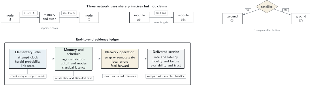
A network claim closes several ledgers at once. Elementary success probability and link fidelity determine stochastic arrivals; memory, scheduling, and classical latency determine which arrivals remain usable; swapping or gate teleportation determines the delivered state; and the application fixes the relevant quality, latency, trust, and comparison benchmark. A laboratory swap, a repeater service, a distributed processor, and a satellite link can share components without establishing the same claim.

Keep the layers separate

Layer	Input and output	Quantities that must remain visible
physical channel	emitted carrier to received optical or microwave mode	attenuation, background, mode overlap, polarization or phase drift, pointing
link generation	node states and photons to a heralded neighboring pair	attempt rate, success probability, false heralds, conditional state, raw duty factor
memory and scheduler	asynchronous link arrivals to simultaneously usable resources	storage efficiency, age distribution, cutoff, queue policy, multiplexing, crosstalk
network operation	neighboring resources to a longer pair, graph state, or remote gate	Bell-measurement success, local-operation error, feed-forward latency, consumed pairs
application	delivered resource to task output	teleportation or gate fidelity, secret-key rate, sensing utility, workload success

The same optical detection can appear in several denominators. It may count as a detector click at the physical layer, a successful herald at the link layer, or one accepted event in an application data set. Reporting must state which one.

Elementary-Link Accounting

A two-photon midpoint link

Consider nodes separated by one elementary length $L_0$. Each node emits a photon entangled with a stationary qubit, and the photons travel to a midpoint Bell-state analyzer. Define the accepted single-arm probability

$$q_i = p_{{\rm em},i} \eta_{{\rm col},i} \eta_{{\rm conv},i} \eta_{{\rm ch},i} \eta_{{\rm det},i}.$$

The factors represent emission into the desired transition, collection into the accepted mode, frequency conversion when present, propagation, and detection. If $p_{\rm BSM}$ is the probability that the analyzer identifies an accepted Bell outcome once both photons arrive, then

$$p_{\rm link} \simeq p_{\rm BSM}q_Aq_B.$$

For a symmetric midpoint link, each half-channel has transmissivity $\sqrt{\eta_0}$, where $\eta_0$ is the transmissivity across $L_0$. Collecting the nonchannel factors into $q_{\rm loc}$ gives

$$p_{\rm link} \simeq p_{\rm BSM} q_{\rm loc}^{\,2} \eta_0.$$

The square on local efficiency is consequential: a modest improvement at each node can change the two-photon rate substantially. Conversely, a quoted detector efficiency does not substitute for end-to-end $q_{\rm loc}$. Linear-optical Bell measurements, detector number resolution, auxiliary photons, and encoding determine $p_{\rm BSM}$; it should not automatically be set to one.

Single-photon heralding protocols use a different probability model. They can replace the coincidence of two transmitted photons by one detection and therefore improve loss scaling for an elementary link, but weak excitation, double emission, optical phase stabilization, and which-path information then enter the fidelity–rate tradeoff. A case study must use the probability model of the implemented protocol rather than borrowing the most favorable factor from another architecture.

Attempts, heralds, and latency

Let $\tau_0$ be the interval between statistically independent attempts, including reset, emission, propagation, detection, and any classical acknowledgement needed before a memory can be reused. With independent attempts, the number $N$ required for one success is geometric:

$$\Pr(N=n) = (1-p_{\rm link})^{n-1}p_{\rm link}, \qquad \mathbb E[N] = \frac{1}{p_{\rm link}}.$$

The idealized mean establishment time is therefore

$$\mathbb E[T_{\rm link}] = \frac{\tau_0}{p_{\rm link}}.$$

This expression is a starting point, not a complete rate. Dead time, periodic cooling, source reloading, detector recovery, phase-lock interruptions, finite acquisition windows, and retry limits all reduce the delivered rate. The full latency distribution matters when a memory expires or a computation waits for a network resource.

Classical signaling also imposes a floor. In fiber with group velocity $v_g$, a heralding pattern whose decision and acknowledgement span a distance $L_h$ requires at least

$$\tau_{\rm cl} \ge \frac{L_h}{v_g} +\tau_{\rm proc}.$$

The exact factor of one or two depends on where detection occurs and where the next decision must be known. Stating merely “the link is $L_0$ long” is not enough to infer the control latency.

The direct-transmission benchmark

For a pure-loss bosonic channel with transmissivity $\eta$, the repeaterless two-way assisted capacity is

$$K_{\rm direct}(\eta) = -\log_2(1-\eta) \simeq \frac{\eta}{\ln 2}$$

bits per optical mode at high loss. This Pirandola–Laurenza–Ottaviani–Banchi bound is a fundamental reference for direct entanglement distribution and secret-key generation over that channel model.

Beating a particular direct-transmission apparatus is useful engineering evidence. Beating the repeaterless bound under matched channel uses, modes, directions, and trust assumptions is a stronger statement. Neither follows from demonstrating a memory or an intermediate node. A fair comparison also keeps source clocks, parallel spectral or spatial modes, and unsuccessful attempts in the resource denominator.

Repeater Accounting Used in These Case Studies

A three-node chain needs independently generated neighboring links to be usable at the same time before the middle node can connect them. That sentence hides the central system variables: geometric waiting times, the age of the earlier link, timeout policy, effective multiplexing, swap recovery, and the difference between a conditional herald and a delivered endpoint state.

Quantum Repeaters derives the exact two-link waiting and age formulas, the many-link asymptotic, cutoff and multiplexing relations, nested schedules, error-control generations, and the event-driven state needed for rate simulation. The case studies below use those results as an accounting contract rather than duplicating their derivations.

For each experiment, keep at least these observations separate:

• every elementary attempt and optical mode launched;
• online heralds, false heralds, and the states left in named memories;
• memory ages and retrieval losses when two links become jointly usable;
• swap outcomes, Pauli-frame updates, failed-operation recovery, and local error;
• endpoint states above the advertised quality threshold;
• sustained delivered rate, latency distribution, availability, and the matched direct benchmark.

Entanglement Swapping owns the Bell-state composition and swap-noise examples, while Quantum Memories owns the age-dependent write–store–read channel. This page asks which of those layers was operated together and what conclusion the resulting evidence supports.

Case Study 1: From a Swap Event to a Three-Node Chain

Photonic entanglement swapping

Pan and co-workers’ 1998 experiment used two polarization-entangled photon pairs. One photon from each pair entered a Bell-state measurement; conditioned on the relevant four-photon detection pattern, the two photons that had not interacted exhibited entanglement. This was the first experimental realization of entanglement swapping.

The result established the physical projection at the heart of swapping. It did not establish a repeater service:

• the endpoint photons were measured rather than stored as on-demand node resources;
• accepted events were conditioned on multi-photon coincidences;
• the experiment did not synchronize independently heralded elementary links with long-lived memories;
• no repeated multi-segment service or direct-transmission rate advantage was claimed.

Those caveats do not diminish the experiment. They identify its exact evidence label: protocol primitive demonstrated.

A three-node solid-state network

Pompili and co-workers reported a three-node network in 2021 using nitrogen-vacancy centers in diamond. Optically active electron spins served as communication qubits, a nuclear spin supplied memory at the middle node, and a phase-stabilized photonic architecture generated neighboring entanglement. Real-time classical control and feed-forward supported entanglement swapping without selecting only favorable outcomes after the entire protocol. The same network distributed a genuine tripartite entangled state.

This result closed several loops absent from a photonic swap event:

1. an $A$–$B$ pair was generated and moved to memory at $B$;
2. the memory was protected while $B$–$C$ generation was attempted;
3. local logic and readout at $B$ performed the swap;
4. feed-forward identified the endpoint Bell state;
5. a network control stack coordinated the nodes.

The physical separations and rates remained laboratory scale. The result was a multi-node network and swapping demonstration, not evidence of metropolitan-distance repeater advantage.

Teleporting through the non-neighboring nodes

Hermans and co-workers extended the platform in 2022. The network first prepared an entangled state between non-neighboring nodes $A$ and $C$ by generating the two neighboring links and swapping at $B$. An input state at $C$ was then teleported to $A$ with real-time feed-forward.

For six cardinal input states, the reported conditional average fidelity was $0.702(11)$ at one event per $117\ {\rm s}$. The experiment also accepted every Bell-measurement outcome in an unconditional mode and reported $0.688(10)$ at one event per $100\ {\rm s}$ for the selected detection window. Both values exceeded the qubit measure-and-prepare benchmark of $2/3$ within the reported uncertainties.

The comparison between conditional and unconditional operation is instructive. “Unit efficiency” at the input of a prepared teleporter means every inserted state is processed; it does not mean that preparing the teleporter had unit probability or zero waiting time. The pre-distributed entanglement, memory protection, control messages, and failed link attempts remain in the service ledger.

Milestone	What it established	What it did not establish
Pan et al. (1998)	conditional photonic swapping primitive	stored or repeated network service
Pompili et al. (2021)	three stationary nodes, memory-assisted swapping, real-time control	long-distance or repeater-rate advantage
Hermans et al. (2022)	teleported qubit across non-neighboring matter nodes	scalable throughput or fault-tolerant network

Case Study 2: A Basic Memory-Assisted Repeater

Protocol skeleton

For three nodes $A$–$B$–$C$, a first-generation elementary repeater cycle is:

1. repeatedly attempt heralded $A$–$B$ entanglement;
2. store the successful pair in a memory at $B$;
3. repeatedly attempt $B$–$C$ entanglement while protecting the first pair;
4. when both links satisfy an age and quality policy, perform a Bell measurement at $B$;
5. communicate the swap outcome and update the endpoint Pauli frame;
6. verify, consume, distill, or deliver the $A$–$C$ pair;
7. regenerate resources after a timeout or failed swap.

Parallel generation changes steps 1–3 but not the need to synchronize. Nested repeaters apply the same idea at several length scales. Entanglement Distillation uses multiple pairs to improve quality probabilistically while accounting for acceptance, raw-pair yield, and local noise. Error-corrected repeaters replace some two-way heralding or purification with encoded operations and one-way processing, at much higher local-resource cost.

The nested scaling argument, three-generation taxonomy, rate model, and event-driven scheduler are developed in Quantum Repeaters. For an evidence audit here, a compact rate claim still has to count every attempt, memory cutoff, consumed pair, failed swap, reset, calibration period, and unavailable interval. Average component probabilities cannot replace the joint distribution of age, quality, controller state, and application latency.

Component milestones are not a complete chain

Several experiments have attacked different repeater bottlenecks:

• Lago-Rivera and co-workers (2021) heralded entanglement between two multimode solid-state memories at rates up to $1.4\ {\rm kHz}$, with predetermined storage up to $25\ \mu{\rm s}$ and $62$ temporal modes.
• Knaut and co-workers (2024) entangled nanophotonic diamond memory nodes through $40\ {\rm km}$ fiber spools and a $35\ {\rm km}$ deployed urban loop, combining telecom conversion, second-scale nuclear-spin storage, and integrated error detection.
• Liu and co-workers (2026) generated remote trapped-ion memory entanglement through $10\ {\rm km}$ of spooled fiber that survived beyond the average establishment time. They also extended elementary-link tests to $101\ {\rm km}$ and analyzed a device-independent key rate.

Each is major repeater-enabling evidence. None by itself is a universal multi-segment repeater chain. In particular, the 2026 result crosses the important inequality

$$T_{\rm useful} > \mathbb E[T_{\rm link}]$$

for the reported $10\ {\rm km}$ configuration, but a complete chain still requires at least two simultaneously usable links, a swap, end-to-end quality and rate accounting, and comparison with a direct benchmark.

What would establish a repeater service?

A strong repeater claim should provide:

1. at least two elementary segments with intermediate quantum resources;
2. online heralding and storage rather than retrospective coincidence selection;
3. swapping, purification, or error correction that changes end-to-end scaling or service quality;
4. raw and delivered rates with every attempted mode counted;
5. end-to-end fidelity or task performance without unsupported background subtraction;
6. memory-age and latency distributions;
7. a direct-transmission comparison under matched channel resources;
8. sustained operation, calibration overhead, and uncertainty.

An intermediate laboratory does not automatically make a link a repeater. Trusted classical key relays, twin-field QKD measurement stations, optical amplifiers, and postselected swapping experiments have different trust and resource models.

Case Study 3: A Modular Quantum-Computer Link

Entanglement as an intermodule instruction

Suppose two processor modules contain circuit qubits $a$ and $b$ plus network qubits $A$ and $B$. A heralded optical protocol prepares a Bell pair on $AB$. Local gates, measurements, classical messages, and Pauli-frame updates can then implement a nonlocal entangling gate on $ab$. In a common gate teleportation construction, one remote controlled-$Z$ consumes one Bell pair and two classical bits.

Distributed Quantum Computing owns the remote-gate derivation, teledata–telegate choice, partitioning, compiler/runtime semantics, and logical resource accounting. This case study owns the experimental evidence and matched comparison.

The important ordering is

$$\text{generate and verify Bell pair} \longrightarrow \text{admit remote instruction} \longrightarrow \text{local gates and measurements}.$$

Photon loss during pair generation can trigger another attempt without destroying the circuit-qubit inputs. Once a qualifying pair is buffered, the logical instruction can be deterministic with respect to that resource. This is stronger than a remote gate whose success is known only after the data qubits have been measured or lost.

The 2025 trapped-ion demonstration

Main and co-workers connected two trapped-ion modules with photons. Each module separated a strontium network qubit from calcium circuit and auxiliary qubits. Photons from the network qubits interfered at a Bell-state analyzer, while dynamical decoupling protected circuit states during stochastic entanglement generation.

The reported elementary-link figures were:

Quantity	Reported value	Role in the system
duration per optical attempt	$1.168\ \mu{\rm s}$	physical trial clock
mean attempts per herald	$7084$	stochastic link overhead
net entanglement rate with recooling	$9.7\ {\rm s}^{-1}$	available Bell-resource rate
Bell-state fidelity	$96.89(8)\%$	network-resource quality
circuit-memory process fidelities during generation	$98.1(4)\%$, $98.2(5)\%$	data survival while waiting
teleported controlled-$Z$ fidelity	$86\%$	remote instruction quality

The rate is lower than the inverse of attempt duration divided by mean attempts because entanglement bursts were interleaved with sympathetic recooling. That gap is precisely why a complete duty-factor ledger matters.

The experiment repeatedly executed teleported nonlocal gates and distributed circuits, including a two-qubit Grover search across the modules. It therefore demonstrated a small distributed processor, not merely remote entanglement. It did not establish that adding modules improves logical reliability or application throughput at scale.

Remote-gate quality and throughput

For small, approximately stochastic errors, an orienting budget is

$$r_{\rm remote} \approx r_{\rm Bell} +r_{{\rm local},A} +r_{{\rm local},B} +r_{\rm mem} +r_{\rm meas} +r_{\rm ff}.$$

Here $r=1-F$ must use compatible fidelity conventions. The sum is not a general theorem: coherent and correlated errors can add constructively or cancel, and leakage is not captured by one depolarizing number. A process matrix or logical error model is needed for prediction.

Throughput has a separate bottleneck:

$$R_{\rm remote} \le \min \left( \frac{R_{\rm Bell}}{n_{\rm Bell}}, R_{\rm local}, R_{\rm controller}, R_{\rm decoder} \right).$$

An application may require Bell pairs faster than they can be generated, or it may be limited by local gates while network pairs wait and decohere. Schedulers therefore need resource reservations, age-aware buffers, backpressure, and a declared policy for stale pairs.

The distinction from a long-distance communication network is architectural. Two separated modules operated under one compiler and controller can form one machine. A wide-area network serves independent endpoints, changing users, routing, security domains, and asynchronous requests. The physical Bell-pair primitive can be similar while the service contract is not.

Case Study 4: Satellite and Free-Space Links

Why free space changes the loss geometry

Fiber transmissivity decreases exponentially with path length:

$$\eta_{\rm fib}(L) = 10^{-\alpha L/10}.$$

In a diffraction-limited free-space link, geometric collection instead decreases approximately as an inverse square once the beam is much larger than the receiver. For a Gaussian beam of radius $w(R)$ and receiver aperture radius $a$,

$$\eta_{\rm geo} = 1- \exp \left[ -\frac{2a^2}{w^2(R)} \right] \simeq \frac{2a^2}{w^2(R)}$$

when $a\ll w(R)$. A link budget may be written

$$\eta_{\rm fs} = \eta_{\rm tx} \eta_{\rm atm} \eta_{\rm point} \eta_{\rm geo} \eta_{\rm rx} \eta_{\rm det}.$$

Atmospheric absorption and scattering, turbulence, beam wander, background light, pointing error, receiver field of view, synchronization, and weather all sit outside the ideal inverse-square picture. An uplink usually suffers more from turbulence near the transmitter than a downlink whose beam crosses the dense atmosphere near the end of propagation.

For an entangled-pair source on a satellite with two downlinks,

$$R_{\rm coinc} \simeq R_{\rm src} \eta_A \eta_B P_{\rm win} P_{\rm accept},$$

where $P_{\rm win}$ accounts for timing acceptance and $P_{\rm accept}$ for basis, background, and quality criteria. Both downlinks must be simultaneously visible, so orbital geometry and common weather become part of the rate.

The Micius demonstrations

In 2017, Yin and co-workers distributed members of entangled photon pairs from the Micius satellite to two ground stations separated by $1203\ {\rm km}$. The two downlinks had a combined optical path varying from about $1600$ to $2400\ {\rm km}$. The experiment observed Bell-inequality violation $S=2.37\pm0.09$ under its space-like-separation arrangement. The reported coincidence rate was about $1.1\ {\rm s}^{-1}$ across total dual-link loss of roughly $64$–$82\ {\rm dB}$.

Companion experiments established different services:

• Liao and co-workers performed satellite-to-ground decoy-state QKD over distances up to $1200\ {\rm km}$ at kilohertz key rates during suitable passes.
• Ren and co-workers teleported six independent photonic input states from a ground station to the satellite over distances up to $1400\ {\rm km}$, reporting average fidelity $0.80\pm0.01$.
• Yin and co-workers later used satellite-distributed entanglement for QKD between ground stations separated by $1120\ {\rm km}$, reporting a finite secret-key rate of $0.12\ {\rm bit\,s^{-1}}$ without a trusted relay.

These are not interchangeable records. Entanglement distribution, prepare-and-measure QKD, teleportation, and entanglement-based QKD have different sources, endpoint trust, classical processing, and output metrics.

A satellite is not automatically a quantum repeater

A satellite carrying an entangled-photon source distributes a bipartite resource through two lossy channels. A satellite that separately establishes keys with two stations and classically relays them is a trusted node. Neither operation necessarily stores an unknown quantum state, synchronizes adjacent quantum links, or performs swapping.

A genuine satellite repeater would need an explicit intermediate quantum resource, such as on-board memory and Bell measurement, or a memory-assisted ground architecture whose online operations change end-to-end scaling. Its service model would also need to include:

• finite pass windows and revisit time;
• day, night, cloud, turbulence, and background constraints;
• acquisition, pointing, and tracking latency;
• orbital ephemeris and handoff among ground stations;
• radiation, thermal cycling, launch, and maintenance constraints;
• authenticated classical control and the satellite trust boundary.

The dramatic geographic baseline is only one coordinate of the network problem.

Comparing the Four Cases

Case	Delivered object	Dominant stochastic resource	Quality bottleneck	Strongest supported label
photonic swap	conditional endpoint photon correlations	multi-photon coincidence	source purity, interference, detector pattern	swapping primitive
three-node matter network	stored endpoint pair or teleported qubit	two heralded links plus memory wait	optical phase, readout, memory under attempts	multi-node protocol
memory-assisted repeater	end-to-end pair above a service threshold	synchronized links, retries, cutoff	memory age, swaps, local operations	architecture until end-to-end benchmarked
modular computer link	remote gate on retained circuit data	buffered Bell-pair arrival	Bell quality plus local gate and memory errors	small distributed computation
satellite free-space link	photons, entanglement, teleported state, or key	channel visibility and dual-link loss	pointing, background, atmosphere, source	long-baseline link or application

No single scalar orders all cases. Distance favors satellite links; duty cycle can favor fiber. Conditional fidelity can favor rare accepted events; throughput can favor a noisier high-rate interface. A distributed computer may value deterministic admission and low tail latency more than geographic range. A cryptographic network must include security and authentication assumptions absent from an entanglement-rate comparison.

Control Plane, Routing, and Cut Limits

Quantum data do not remove the need for classical networking. A functioning service carries:

• attempt identifiers and synchronized clock labels;
• detector outcomes and herald validity;
• memory addresses, ages, and quality estimates;
• Bell-measurement outcomes and Pauli-frame updates;
• routing, reservation, timeout, and retry decisions;
• calibration versions and reference-frame corrections;
• application acknowledgements and audit records.

These messages have latency, loss, ordering, and security requirements. Applying a correction to the wrong time bin or reusing a memory before a late herald arrives is a protocol failure, not merely classical overhead.

Network topology also imposes cut limits. If an end-to-end task must cross a cut $\mathcal C$ of a graph and each edge $e$ has an assisted capacity $C_e$, an upper-bound structure is

$$C_{\rm end} \le \min_{\mathcal C} \sum_{e\in\mathcal C} C_e$$

under the specified routing and channel-use model. For a single path, its bottleneck edge limits asymptotic flow. Multipath routing can add capacity across a cut, but only when sources, memories, switches, and endpoint consumption can exploit the paths concurrently.

Entanglement fidelity introduces another routing dimension. The shortest path need not maximize delivered rate or quality. An age-aware router may prefer a longer path with fresh high-fidelity pairs over a nominally short path whose memories are near cutoff. The routing metric must therefore be derived from the application contract, not imported unchanged from classical packet networks.

Evidence Ladder

Network evidence becomes progressively stronger:

1. component characterization: source, detector, memory, converter, or local gate measured at a declared reference plane;
2. elementary quantum link: remote entanglement or state transfer between two nodes with online heralding;
3. network primitive: swapping, purification, routing, or remote gate completed with real-time control;
4. multi-node service: requested states delivered to named endpoints through an interface over repeated trials;
5. application result: teleportation, computation, key generation, or sensing validated end to end;
6. scaling evidence: rate, quality, latency, or logical reliability improves under added distance, nodes, or resources against a matched baseline;
7. operational evidence: sustained availability, autonomous calibration, security, maintainability, and reproducibility in the intended environment.

Later rungs do not make early rungs obsolete. They answer different questions. A component record can be scientifically important without showing application value; an application demonstration can work at small scale without establishing favorable scaling.

Common Mistakes

• Calling every intermediate optical station a quantum repeater.
• Multiplying link success probabilities when memories allow asynchronous successes to be synchronized.
• Ignoring the maximum of stochastic waiting times and the age of the first stored pair.
• Reporting conditional fidelity without herald probability, false-herald rate, or delivered throughput.
• Treating memory $T_2$ as the usable network storage time without write, read, and repeated-attempt noise.
• Calling postselected coincidence analysis an on-demand network service.
• Describing a gate as deterministic while omitting stochastic preparation of its entanglement resource.
• Comparing rates per second while hiding different source clocks, mode counts, or parallel channels.
• Treating geographic distance, fiber length, optical path, and node separation as the same quantity.
• Calling a trusted satellite key relay an untrusted entanglement repeater.
• Quoting a direct-transmission comparison without specifying whether it is an experimental baseline or a fundamental capacity bound.
• Inferring scalable operation from one successful multi-node sequence.

Reporting Checklist

A mature network report should include:

1. Topology: node locations, physical path lengths, logical edges, and trusted boundaries.
2. Requested service: endpoint state or operation, quality threshold, latency objective, availability, and failure parameter.
3. Attempt denominator: source clock, attempted modes, parallel resources, rejected attempts, and dead time.
4. Link characterization: end-to-end success, false heralds, conditional state, and drift at fixed settings.
5. Memory characterization: write and read efficiency, age-dependent channel, cutoff, and noise during repeated link attempts.
6. Network operations: swap or remote-gate process, outcome dependence, feed-forward, consumed resources, and recovery after failure.
7. Delivered metrics: raw and thresholded rate, latency distribution, fidelity or task output, uncertainty, and uptime.
8. Comparison: matched direct link, repeaterless capacity, prior architecture, or classical application baseline.
9. Control and security: synchronization, authenticated messages, calibration version, operator intervention, and threat model.
10. Evidence label: demonstrated, simulated from measured components, projected, or required by a future architecture.

Reporting Standards develops the broader provenance and uncertainty requirements. Claims, Hype, and Evidence Standards provides the canonical vocabulary for separating demonstrations from projections.

Exercises

Exercises 2, 3, and 5 apply the timing, cutoff, and multiplexing relations derived in Quantum Repeaters. Exercise 4 uses the Bell-diagonal swap model developed in Entanglement Swapping.

1. Elementary two-photon link

Two nodes are separated by $50\ {\rm km}$ of fiber with attenuation $0.2\ {\rm dB\,km^{-1}}$. For each arm, the product of emission, collection, conversion, and detection efficiencies excluding channel loss is $q_{\rm loc}=0.25$. A midpoint linear-optical analyzer accepts a Bell outcome with probability $p_{\rm BSM}=1/2$. Find $p_{\rm link}$ per attempt. If attempts occur every $250\ \mu{\rm s}$, find the idealized mean link time.

Solution

The total transmissivity across the elementary length is

$$\eta_0 = 10^{-0.2(50)/10} = 0.1.$$

Each half contributes $\sqrt{\eta_0}$, so the product of the two arms contains $\eta_0$. Therefore

$$p_{\rm link} = \frac12(0.25)^2(0.1) = 3.125\times10^{-3}.$$

The mean number of attempts is $320$, giving

$$\mathbb E[T_{\rm link}] = 320(250\ \mu{\rm s}) = 80\ {\rm ms}.$$

This omits reset failures, stabilization downtime, false-herald filtering, and any extra classical-control interval.

2. Waiting for two links

Two links are attempted in parallel with $p=0.01$ per cycle and $\tau_0=100\ \mu{\rm s}$. Compute the exact mean time until both are ready and the mean age of the first pair when the second arrives.

Solution

For the maximum of two geometric waiting times,

$$\mathbb E[N_{\max}] = \frac{3-2p}{p(2-p)} = \frac{2.98}{0.0199} \approx 149.75.$$

Thus the mean preparation time is about

$$14.98\ {\rm ms}.$$

The mean waiting-time difference is

$$\mathbb E[|N_1-N_2|] = \frac{2(1-p)}{p(2-p)} = \frac{1.98}{0.0199} \approx 99.50.$$

The first pair is therefore about $9.95\ {\rm ms}$ old on average when both links are ready. This age, not just the total preparation time, enters its memory channel.

3. A memory-age cutoff

A stored Bell pair has visibility $v(t)=0.96\exp[-t/(20\ {\rm ms})]$. The application requires $F\ge0.80$ under the Werner model. Find the latest acceptable age.

Solution

The Werner relation gives the minimum visibility

$$v_{\min} = \frac{4F_{\min}-1}{3} = \frac{2.2}{3} \approx 0.7333.$$

Set $0.96e^{-t_c/(20\ {\rm ms})}=0.7333$:

$$t_c = -20\ {\rm ms} \ln \left( \frac{0.7333}{0.96} \right) \approx 5.39\ {\rm ms}.$$

A scheduler using a longer cutoff may improve raw coincidence rate but would deliver pairs below the stated fidelity threshold in this model.

4. Fidelity after swapping

Two Werner links have fidelities $F_1=0.92$ and $F_2=0.90$. Model the swap by visibility $v_s=0.97$. Find the output fidelity.

Solution

Convert fidelity to visibility:

$$v_1 = \frac{4F_1-1}{3} \approx 0.8933, \qquad v_2 \approx 0.8667.$$

Then

$$v_{\rm out} = v_s v_1v_2 \approx 0.7509,$$

and

$$F_{\rm out} = \frac{1+3v_{\rm out}}{4} \approx 0.813.$$

Multiplying the input fidelities directly would give the wrong model.

5. Multiplexing gain

An elementary mode succeeds with probability $p=2\times10^{-4}$ per cycle. Compute the probability of at least one success with $M=100$ independent modes. Compare it with the linear approximation.

Solution

The exact probability is

$$p_M = 1-(1-p)^{100} \approx 1-(0.9998)^{100} \approx 0.01980.$$

The linear approximation gives

$$Mp = 0.02000.$$

The approximation is accurate here because $Mp=0.02\ll1$. The calculation assumes independent, simultaneously usable modes and does not include shared switching or detector limits.

6. Remote-gate error budget

A distributed-gate model assigns infidelities $0.031$ to the Bell resource, $0.020$ and $0.024$ to the two local couplings, $0.015$ to memory while waiting, and $0.010$ to measurement and feed-forward. Estimate the remote gate fidelity using a first-order stochastic budget. Why is this only an estimate?

Solution

The first-order infidelity is

$$r_{\rm remote} \approx 0.031+0.020+0.024+0.015+0.010 = 0.100.$$

Thus

$$F_{\rm remote} \approx 0.900.$$

The estimate assumes compatible fidelity definitions and small independent stochastic errors. Coherent errors, correlations, leakage, outcome dependence, and higher-order terms require channel composition or process tomography.

7. Free-space aperture capture

A downlink beam has radius $w=5.0\ {\rm m}$ at a circular receiver of radius $a=0.50\ {\rm m}$. Estimate $\eta_{\rm geo}$ exactly in the Gaussian model and by the small-aperture approximation. If all other efficiencies multiply to $0.12$, find the total detection probability per transmitted photon.

Solution

The exact geometric capture is

$$\eta_{\rm geo} = 1-\exp \left[ -\frac{2(0.50)^2}{(5.0)^2} \right] = 1-e^{-0.02} \approx 0.01980.$$

The approximation gives

$$\eta_{\rm geo} \simeq \frac{2(0.50)^2}{(5.0)^2} = 0.02000.$$

The total detection probability is

$$\eta_{\rm fs} \approx 0.12(0.01980) \approx 2.38\times10^{-3}.$$

Pointing fluctuations change the time distribution of this probability and cannot always be represented by one constant factor.

8. Classify the claim

An experiment entangles two memories through $40\ {\rm km}$ of fiber with online heralding and second-scale storage. It uses no second elementary link and performs no swap. Which evidence labels are justified, and what minimum additional demonstration would support a three-node repeater claim?

Solution

The experiment justifies elementary quantum link, remote memory–memory entanglement, and repeater-enabling component labels. It does not yet justify an end-to-end repeater service.

At minimum, a three-node claim needs two independently generated neighboring links, simultaneous usable storage, an online swap or error-corrected connection at the middle node, and characterization of the delivered endpoint state. A strong repeater-performance claim additionally needs rate, latency, memory-age, channel-use, and matched direct-transmission comparisons.

Further Connections

• Communication with Quantum Systems supplies the operational task and rate language used to compare direct, repeater-assisted, and distributed-computing services.
• Negative Results and Limitations develops the repeaterless pure-loss bound and the distinction between an enabling component, a direct-link benchmark, and a delivered network advantage.
• Claims and Evidence Checklist supplies the practical comparator, provenance, and bounded-disposition audit for a network claim.

References

1. M. Żukowski, A. Zeilinger, M. A. Horne, and A. K. Ekert, “Event-ready-detectors Bell experiment via entanglement swapping,” Physical Review Letters 71, 4287–4290 (1993), doi:10.1103/PhysRevLett.71.4287.
2. J.-W. Pan, D. Bouwmeester, H. Weinfurter, and A. Zeilinger, “Experimental entanglement swapping: Entangling photons that never interacted,” Physical Review Letters 80, 3891–3894 (1998), doi:10.1103/PhysRevLett.80.3891.
3. H.-J. Briegel, W. Dür, J. I. Cirac, and P. Zoller, “Quantum repeaters: The role of imperfect local operations in quantum communication,” Physical Review Letters 81, 5932–5935 (1998), doi:10.1103/PhysRevLett.81.5932.
4. L.-M. Duan, M. D. Lukin, J. I. Cirac, and P. Zoller, “Long-distance quantum communication with atomic ensembles and linear optics,” Nature 414, 413–418 (2001), doi:10.1038/35106500.
5. H. J. Kimble, “The quantum internet,” Nature 453, 1023–1030 (2008), doi:10.1038/nature07127.
6. N. Sangouard, C. Simon, H. de Riedmatten, and N. Gisin, “Quantum repeaters based on atomic ensembles and linear optics,” Reviews of Modern Physics 83, 33–80 (2011), doi:10.1103/RevModPhys.83.33.
7. S. Muralidharan et al., “Optimal architectures for long distance quantum communication,” Scientific Reports 6, 20463 (2016), doi:10.1038/srep20463.
8. S. Pirandola et al., “Fundamental limits of repeaterless quantum communications,” Nature Communications 8, 15043 (2017), doi:10.1038/ncomms15043.
9. S. Wehner, D. Elkouss, and R. Hanson, “Quantum internet: A vision for the road ahead,” Science 362, eaam9288 (2018), doi:10.1126/science.aam9288.
10. S. Pirandola, “End-to-end capacities of a quantum communication network,” Communications Physics 2, 51 (2019), doi:10.1038/s42005-019-0147-3.
11. L. Stephenson et al., “High-rate, high-fidelity entanglement of qubits across an elementary quantum network,” Physical Review Letters 124, 110501 (2020), doi:10.1103/PhysRevLett.124.110501.
12. M. Pompili et al., “Realization of a multinode quantum network of remote solid-state qubits,” Science 372, 259–264 (2021), doi:10.1126/science.abg1919.
13. D. Lago-Rivera et al., “Telecom-heralded entanglement between multimode solid-state quantum memories,” Nature 594, 37–40 (2021), doi:10.1038/s41586-021-03481-8.
14. S. Daiss et al., “A quantum-logic gate between distant quantum-network modules,” Science 371, 614–617 (2021), doi:10.1126/science.abe3150.
15. S. L. N. Hermans et al., “Qubit teleportation between non-neighbouring nodes in a quantum network,” Nature 605, 663–668 (2022), doi:10.1038/s41586-022-04697-y.
16. T. van Leent et al., “Entangling single atoms over 33 km telecom fibre,” Nature 607, 69–73 (2022), doi:10.1038/s41586-022-04764-4.
17. C. M. Knaut et al., “Entanglement of nanophotonic quantum memory nodes in a telecom network,” Nature 629, 573–578 (2024), doi:10.1038/s41586-024-07252-z.
18. A. J. Stolk et al., “Metropolitan-scale heralded entanglement of solid-state qubits,” Science Advances 10, eadp6442 (2024), doi:10.1126/sciadv.adp6442.
19. D. Main et al., “Distributed quantum computing across an optical network link,” Nature 638, 383–388 (2025), doi:10.1038/s41586-024-08404-x.
20. W.-Z. Liu et al., “Long-lived remote ion–ion entanglement for scalable quantum repeaters,” Nature 652, 51–57 (2026), doi:10.1038/s41586-026-10177-4.
21. J. Yin et al., “Satellite-based entanglement distribution over 1200 kilometers,” Science 356, 1140–1144 (2017), doi:10.1126/science.aan3211.
22. S.-K. Liao et al., “Satellite-to-ground quantum key distribution,” Nature 549, 43–47 (2017), doi:10.1038/nature23655.
23. J.-G. Ren et al., “Ground-to-satellite quantum teleportation,” Nature 549, 70–73 (2017), doi:10.1038/nature23675.
24. J. Yin et al., “Entanglement-based secure quantum cryptography over 1,120 kilometres,” Nature 582, 501–505 (2020), doi:10.1038/s41586-020-2401-y.
25. D. Hucul et al., “Modular entanglement of atomic qubits using photons and phonons,” Nature Physics 11, 37–42 (2015), doi:10.1038/nphys3150.
26. D. Gottesman and I. L. Chuang, “Demonstrating the viability of universal quantum computation using teleportation and single-qubit operations,” Nature 402, 390–393 (1999), doi:10.1038/46503.
27. A. Reiserer and G. Rempe, “Cavity-based quantum networks with single atoms and optical photons,” Reviews of Modern Physics 87, 1379–1418 (2015), doi:10.1103/RevModPhys.87.1379.