Materials Simulation Case Studies

Short Definition

A materials-simulation case study follows a declared material question through model construction, finite-instance selection, quantum implementation, observable estimation, validation, and comparison with the best relevant classical methods. The phrase covers several scientifically different tasks:

• studying an idealized many-body Hamiltonian that captures a mechanism;
• testing whether an effective Hamiltonian describes a real material;
• predicting a material property to useful accuracy;
• estimating the resources that a future fault-tolerant computer would need;
• comparing quantum and classical costs for a fixed computational problem.

Those tasks should not be merged into one generic claim of “simulating a material.” A programmable array that reveals a phase of the Hubbard model may be an important model experiment even when no specific compound is being predicted. Conversely, calculating a useful battery voltage requires more than solving one electronic Hamiltonian: structures, compositions, phases, free-energy corrections, and uncertainty all enter.

What Is Quantum Simulation? owns the general simulation contract and the digital–analog–hybrid taxonomy. Hubbard Model, Heisenberg Model, and Transverse-Field Ising Model own the canonical physics of those models. Hubbard Physics in Materials owns downfolding and the model-to-material bridge. Simulation of Quantum Materials owns the material-to-finite-target-to-processor workflow. This page owns the evidence-centered comparison of representative materials case studies.

Three Claims That Must Be Separated

Simulating a model

The target is a mathematical Hamiltonian with specified geometry, couplings, initial state, and observable. Success means reproducing a prediction of that model within a declared tolerance. The target need not be a literal material. Cold atoms in an optical lattice and Rydberg atoms in tweezer arrays are often used this way: they create clean, controllable realizations of lattice Hamiltonians that expose mechanisms difficult to isolate in solids.

Modeling a material

The target is an effective description of a compound in a specified regime. Success requires evidence that the retained orbitals, couplings, dimensional reduction, disorder model, and omitted interactions are adequate for the observable. Agreement between a simulator and the effective Hamiltonian verifies the simulation; agreement between the effective Hamiltonian and laboratory data validates the material model. Both links matter.

Computing a material property

The output is a quantity used in science or engineering, such as a phase boundary, dynamical structure factor, cell voltage, migration barrier, or reaction free energy. Success requires the complete workflow and propagated uncertainty. An accurate ground-state energy for one fixed geometry may be a kernel inside that workflow, not the final property.

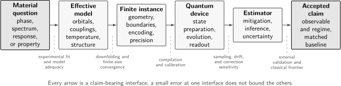
A materials claim crosses several independently fallible interfaces. Device accuracy does not certify the effective model, and model agreement at one parameter point does not establish a useful property calculation. Mature case studies identify the evidence attached to every arrow.

A Layered Error Ledger

Let $O_{\mathrm{lab}}$ be the experimentally defined material observable and let $O_{\mathrm{model}}$ be the exact prediction of the chosen effective model in the intended thermodynamic, continuum, and precision limits. Let $O_L$ be the exact answer for the finite encoded instance, and let $\widehat O$ be the reported quantum estimate. A diagnostic decomposition is

$$\begin{aligned} \widehat O-O_{\mathrm{lab}} ={}& \left( \widehat O-O_{\mathrm{impl}} \right) + \left( O_{\mathrm{impl}}-O_L \right) \\ &+ \left( O_L-O_{\mathrm{model}} \right) + \left( O_{\mathrm{model}}-O_{\mathrm{lab}} \right). \end{aligned}$$

The four terms represent:

1. estimation error: finite shots, readout, drift, mitigation, fitting, and statistical uncertainty;
2. implementation error: imperfect preparation and dynamics relative to the intended finite problem;
3. finite-model error: size, boundaries, discretization, truncation, Trotterization, and requested precision;
4. material-model discrepancy: downfolding, parameters, phonons, disorder, dimensionality, finite temperature, and other omitted physics.

This is an accounting device, not a promise that every contribution is independent or additive. Bias can cancel, mitigation is nonlinear, and an effective model may be calibrated using the same measurements later used for validation. A defensible uncertainty statement records covariance and avoids counting reused data as independent confirmation.

For phase or response claims, a scalar error at one point is rarely enough. One may need a norm over a parameter region,

$$\epsilon_{\mathcal R} = \sup_{\lambda\in\mathcal R} \left| \widehat O(\lambda)-O_{\mathrm{ref}}(\lambda) \right|,$$

or a weighted residual,

$$\chi^2 = \sum_a \frac{ \left[ \widehat O_a-O_a^{\mathrm{exp}} \right]^2 }{ \sigma_{a,\mathrm{q}}^2 + \sigma_{a,\mathrm{exp}}^2 }.$$

The residual is interpretable only when the covariance model, fitted parameters, and held-out validation data are reported.

Case Study 1: Cold-Atom Fermi–Hubbard Experiments

The target model

For spin-$1/2$ fermions on a lattice, a common inhomogeneous Hubbard Hamiltonian is

$$\begin{aligned} H ={}& -\sum_{\langle i,j\rangle,\sigma} t_{ij} \left( c_{i\sigma}^\dagger c_{j\sigma} + c_{j\sigma}^\dagger c_{i\sigma} \right) \\ &+ \sum_i U_i n_{i\uparrow}n_{i\downarrow} + \sum_i \left( V_i-\mu \right)n_i. \end{aligned}$$

Here $t_{ij}$ controls tunneling, $U_i$ the onsite interaction, $V_i$ the confining potential, and $\mu$ the chemical potential. In a quantum-gas microscope, local occupation and spin can be sampled across many experimental preparations. Relevant observables include the double occupancy

$$D_i = \langle n_{i\uparrow}n_{i\downarrow} \rangle$$

and connected spin correlations

$$C_{ij}^{zz} = \langle S_i^zS_j^z\rangle - \langle S_i^z\rangle \langle S_j^z\rangle.$$

The spin structure factor is a spatial Fourier transform,

$$S(\mathbf q) = \frac{1}{N} \sum_{i,j} e^{i\mathbf q\cdot(\mathbf r_i-\mathbf r_j)} C_{ij}^{zz}.$$

The 2017 antiferromagnet

Mazurenko and collaborators prepared a two-dimensional repulsive Fermi–Hubbard system with roughly 80 sites and observed antiferromagnetic correlations extending across the sample. Their quantum-gas microscope resolved local spin and density information, allowing the structure factor, correlation length, and staggered magnetization to be inferred. The reported temperature was in the low-$k_{\mathrm B}T/t$ regime, approximately one quarter in the central region, and antiferromagnetic correlations persisted under moderate hole doping.

This was a scientifically substantial analog-simulation result. It accessed a finite-temperature, doped, two-dimensional regime whose combination of size and sign structure is challenging for many classical methods. It did not, however, constitute a calculation of a cuprate or another specific solid. The implemented optical-lattice Hamiltonian was the target. Mapping the result to a material would additionally require a defensible orbital construction, couplings, longer-range terms, phonons, disorder, interlayer effects, and an observable-level validation argument.

Calibration is central to the evidence. Lattice depths determine $t$ and $U$; the trap makes density and entropy inhomogeneous; imaging has parity and classification errors; and the preparation need not realize a global Gibbs state. Thermometry therefore relies on comparison of selected correlations with controlled numerical or high-temperature results. That is a hybrid validation loop, not a weakness to hide.

Nagaoka polarons in 2024

Lebrat and collaborators used a triangular optical lattice and site-resolved imaging to study mobile dopants in a strongly interacting Fermi–Hubbard system. Particle dopants were surrounded by extended ferromagnetic correlations, while the frustrated geometry produced different, predominantly antiferromagnetic dressing around hole dopants. The experiment provided microscopic evidence for Nagaoka-polaron physics and compared distinct classical calculations with the measured correlation patterns.

The strongest claim is mechanism-level: coherent dopant motion and spin exchange can form extended magnetic polarons in the implemented Hubbard regime. The result does not show that a bulk ferromagnetic material has been designed, and it does not make every doped Hubbard regime classically inaccessible. Geometry, temperature, doping, observable, and benchmark method remain part of the statement.

What these cases establish

Cold-atom Hubbard experiments can:

• realize clean lattice Hamiltonians with tunable interaction and filling;
• measure local correlations unavailable in most bulk probes;
• test finite-temperature many-body methods in controlled regimes;
• discover mechanism-level behavior before a material-specific mapping exists.

They do not automatically establish:

• a quantitative prediction for a named solid;
• a speedup over every classical method;
• the low-temperature thermodynamic limit;
• a complete electronic-structure calculation.

Case Study 2: A 16-Qubit Digital Fermi–Hubbard Calculation

Stanisic and collaborators executed a scalable variational protocol for ground-state observables of $1\times8$ and $2\times4$ spinful Hubbard lattices. Direct occupation encoding used 16 qubits. The workflow combined a free-fermion initial state prepared with Givens rotations, a Hamiltonian-variational circuit, fermionic swap networks, grouped measurements, and error mitigation on superconducting processors.

A Hamiltonian variational family can be written schematically as

$$\lvert\psi(\boldsymbol\theta)\rangle = \prod_{\ell=1}^{p} e^{-i\theta_{\ell,U}H_U} e^{-i\theta_{\ell,h}H_h} \lvert\psi_0\rangle,$$

where $H_h$ contains hopping terms and $H_U$ onsite interactions. Respecting fermionic mode ordering and hardware connectivity is not bookkeeping: fermionic swaps and routing determine a large part of the two-qubit cost.

The experiment reproduced qualitative signatures including interaction-driven changes in double occupancy, density modulation, correlation decay, and antiferromagnetic ordering tendencies. Small exact instances enabled direct comparison. The important qualification is depth. Low-depth circuits retained qualitative structure on hardware, while the authors’ scaling analysis indicated that quantitatively accurate instances beyond routine classical reach would require hundreds of two-qubit layers under the studied approach, well beyond the demonstrated noise budget.

This case establishes an algorithmic hardware run for a finite lattice model. It does not establish a materials prediction or computational advantage. The geometry is small, classical reference answers are available, optimization and mitigation contribute material classical work, and extrapolating a successful shallow circuit to a deep target requires a measured error model.

The case is nevertheless instructive because it exposes the complete near-term bottleneck:

$$\text{useful scale} \Longrightarrow \text{greater depth} \Longrightarrow \text{more noise and mitigation cost} \Longrightarrow \text{weaker validation}.$$

A qubit count alone misses this tension. The accepted-answer tolerance, circuit depth, state overlap, number of observables, shots, optimizer evaluations, and classical baseline all belong in the resource statement.

Case Study 3: Rydberg Spin Models

Programmable Hamiltonian

A common neutral-atom Rydberg model is

$$H = \frac{\hbar\Omega}{2} \sum_i \sigma_i^x - \hbar\Delta \sum_i n_i + \sum_{i<j} V_{ij}n_in_j,$$

with

$$n_i = \frac{1+\sigma_i^z}{2}, \qquad V_{ij} \simeq \frac{C_6}{r_{ij}^6}.$$

After expanding $n_in_j$, this is a long-range Ising-type Hamiltonian with geometry-dependent couplings and longitudinal fields. The atom positions are programmable, which makes square, triangular, frustrated, and irregular graphs experimentally accessible. It is not generally the nearest-neighbor Ising model: interaction tails, boundary fields, missing atoms, Doppler effects, and position uncertainty must be retained or bounded.

Hundreds of atoms

In 2021, Ebadi and collaborators studied quantum phases and dynamics with 64–256 Rydberg atoms. They prepared ordered phases, mapped phase boundaries, and investigated dynamics near the $(2+1)$-dimensional Ising transition. Scholl and collaborators independently simulated two-dimensional antiferromagnets with up to 196 Rydberg atoms in square and triangular geometries, resolving correlations and frustrated ordering.

These experiments are strong examples of programmable model laboratories. Their scientific value does not depend on assigning each atom to an atom in a literal magnetic crystal. They probe phase formation, critical dynamics, frustration, defects, and correlation growth in Hamiltonians whose scale and geometry challenge exact diagonalization.

The relevant validation is observable-specific:

• calibrate $\Omega$, $\Delta$, positions, and the interaction law;
• compare small arrays and short times with exact or controlled numerical calculations;
• test symmetries, conservation laws where applicable, and repeated calibrations;
• report atom loss, preparation defects, readout confusion, and postselection;
• vary size, ramp rate, geometry, and boundary conditions;
• distinguish an equilibrium phase from a finite-rate dynamical pattern.

The nearest classical competitor depends on the regime. Tensor networks can be excellent for low entanglement and favorable geometry; quantum Monte Carlo can be powerful when weights are nonnegative; cluster expansions can control short times or high temperatures; and exact methods remain decisive on small light cones. “Two hundred atoms” is therefore a scale descriptor, not a complexity certificate.

Case Study 4: The 127-Qubit Kicked-Ising Experiment

Kim and collaborators executed Trotterized dynamics for a transverse-field Ising model on the heavy-hex connectivity of a 127-qubit superconducting processor. Across the reported experiments, circuits reached up to 60 layers of two-qubit gates and 2,880 CNOT gates. Pauli twirling, probabilistic error cancellation, and zero-noise extrapolation were used to estimate selected ideal-circuit observables.

The model was

$$H = -J \sum_{\langle i,j\rangle} Z_iZ_j + h \sum_i X_i,$$

and one first-order step has the form

$$U_{\delta t} \approx e^{-ih\delta t\sum_iX_i} e^{iJ\delta t\sum_{\langle i,j\rangle}Z_iZ_j}.$$

The paper deliberately treated the Trotterized circuit as the computational target for its classical comparisons. That choice isolates processor and estimator performance, but it also means that agreement certifies the circuit, not the continuous-time Hamiltonian at arbitrary step size and not a specific material.

The study first used regimes and observables with exact verification, then compared harder cases with available approximate classical methods. Its claim was “evidence for utility,” explicitly not a proven algorithmic speedup. This was a sensible narrower label: the experiment demonstrated controlled expectation-value estimation at notable circuit scale while leaving the classical frontier open.

That frontier moved quickly. Tindall and collaborators developed a belief-propagation tensor-network treatment adapted to the locally tree-like heavy-hex graph. For the same kicked-Ising problem, it produced results more accurate and precise than the quantum estimates and extended the calculation to the thermodynamic limit. Other classical methods also improved.

The lesson is not that the original experiment lacked value. It is that classical baselines are part of a living scientific record. A claim should therefore name:

1. the exact circuit family and observable;
2. the quantum hardware, calibration date, and total sampling cost;
3. every mitigation assumption and correction overhead;
4. the classical algorithms, convergence controls, hardware, and date;
5. whether a later classical result changes only the advantage claim or also the physical conclusion.

Case Study 5: Annealing Dynamics and a Contested Frontier

King and collaborators reported nonequilibrium spin-glass dynamics on superconducting quantum annealers and compared sampled correlations with solutions of the Schrödinger equation. A generic annealing Hamiltonian is

$$H(s) = -A(s) \sum_i X_i + B(s) \left( \sum_i h_iZ_i + \sum_{i<j}J_{ij}Z_iZ_j \right).$$

The 2025 peer-reviewed study considered two-, three-, and infinite-dimensional model geometries, reported area-law entanglement in the quench dynamics, and argued that leading tensor-network and neural-state calculations did not match the annealer’s accuracy within the studied resource budget. The authors described the result as beyond-classical quantum simulation.

That claim is both important and scope-sensitive. Independent classical work using tensor networks and time-dependent variational Monte Carlo reproduced substantial subsets of the benchmark and challenged parts of the inferred frontier. The quantum study and the classical responses differ in geometry, observable order, accuracy target, and which largest instances are covered. As of this review, the broadest claim remains actively contested rather than cleanly reducible to “proved” or “refuted.”

Even if a matched computational advantage is sustained for the full benchmark, another distinction remains: the target is programmable spin-glass quench dynamics, not an end-to-end prediction for a named material. “Scientifically meaningful model problem” and “validated material property” are both valuable labels, but they are not synonyms.

Case Study 6: Direct Comparison with Material Experiments

Two March 2026 preprints moved the evidence boundary from generic model experiments toward direct material validation. Because both were preprints at the review date, their results should be treated as developing evidence rather than settled benchmarks.

Digital dynamical structure factors

Lee and collaborators used a superconducting processor with up to 50 qubits in a quantum–classical workflow for the dynamical structure factor of $\mathrm{KCuF}_3$, a quasi-one-dimensional antiferromagnet with spinon excitations. For spin components $\alpha,\beta$, the target has the form

$$\begin{aligned} S^{\alpha\beta}(\mathbf q,\omega) ={}& \frac{1}{2\pi N} \sum_{j,k} e^{-i\mathbf q\cdot(\mathbf r_j-\mathbf r_k)} \\ &\times \int_{-\infty}^{\infty} dt\, e^{i\omega t} \langle S_j^\alpha(t)S_k^\beta(0) \rangle. \end{aligned}$$

This quantity is directly connected to inelastic neutron-scattering intensity after form factors, polarization factors, resolution, temperature, and normalization are handled. The study compared simulated spectra with laboratory measurements using several metrics and examined how circuit depth and fidelity affected agreement. It also considered a less integrable XXZ chain with next-nearest-neighbor coupling as a model relevant to $\mathrm{CsCoX}_3$ compounds above their ordering temperature.

The methodological advance is the explicit material-to-measurement bridge: the output is not only an abstract circuit expectation value but a spectrum that can be checked against a physical probe. The open questions include peer review, classical comparison in every reported regime, resolution and finite-temperature modeling, and whether increasing system size improves the material prediction rather than only the encoded model.

Analog one-to-one mapping

Leclerc and collaborators used a 256-atom Rydberg simulator to implement an effective two-dimensional model for the layered frustrated magnet $\mathrm{TmMgGaO}_4$. They compared simulator magnetization with independent laboratory measurements, studied the antiferromagnetic transition, connected snapshot observables with integrated neutron data, and explored nonequilibrium response on the corresponding material timescale.

This is stronger evidence than visual similarity between two phase diagrams: material data constrain a declared effective Hamiltonian and the simulator tests that Hamiltonian in a programmable setting. Yet “one-to-one” must still be read operationally. The real crystal has three-dimensional couplings, disorder, phonons, higher crystal-field states, and probe-dependent response; the simulator realizes a selected low-energy model over a selected regime. Agreement validates that model for the tested observables, not every property of the compound.

These preprints illustrate a productive standard for future work:

• identify a material whose effective degrees of freedom match the simulator;
• fit parameters using a declared training subset;
• predict held-out observables or regimes;
• compare against calibrated laboratory data with covariance;
• include the best classical calculation as a third vertex;
• state which discrepancy would falsify the proposed effective model.

Case Study 7: Fault-Tolerant Battery-Material Estimates

Delgado and collaborators developed an end-to-end algorithmic proposal for properties of lithium-ion battery materials and estimated resources for dilithium iron silicate. The quantum kernel uses first-quantized state preparation, qubitization, and phase estimation to obtain periodic ground-state energies. The intended scientific outputs include equilibrium cell voltage, ionic mobility, and thermal stability.

For two lithium compositions $x_1$ and $x_2$, a simplified zero-temperature voltage relation is

$$V = - \frac{ E_{\mathrm{cath}}(x_2) - E_{\mathrm{cath}}(x_1) - (x_2-x_1)E_{\mathrm{Li}} }{ (x_2-x_1)e }.$$

This equation makes the workflow boundary visible. At least three energies enter, and each may require structure optimization, phase selection, finite cells, pseudopotentials or all-electron choices, and error-controlled quantum estimation. At operating temperature, Gibbs free energies and configurational effects replace a simple difference of electronic ground energies.

An ionic migration barrier is likewise an energy difference along a path,

$$E_{\mathrm m} = \max_{\lambda\in[0,1]} E(\mathbf R(\lambda)) - E(\mathbf R_{\mathrm{min}}),$$

so a useful calculation needs enough images to locate the saddle and enough accuracy to resolve the barrier. Thermal stability may require competing decomposition products rather than one cathode energy.

This case is a resource estimate, not a hardware execution. Its value is to connect a fault-tolerant electronic-structure primitive to recognizable materials questions and expose state preparation, precision, and repeated energy calls. Its conclusions are conditional on:

• the first-quantized representation and basis cutoff;
• ground-state overlap and preparation success;
• block-encoding and qubitization costs;
• logical error budget and architecture assumptions;
• the number of structures, compositions, and phases;
• classical preprocessing and postprocessing;
• comparison with improving classical materials methods.

Resource Estimation Tools develops the logical-to-physical compilation and uncertainty sweeps needed before a logical gate count becomes a machine estimate.

Phase Estimation, VQE, or Analog Simulation?

No method wins independently of the task and hardware.

Route	Strength	Dominant cost or limitation	Appropriate evidence
Analog simulation	Native many-body evolution, large arrays, local snapshots	Hamiltonian calibration, restricted programmability, temperature and model mismatch	Cross-platform calibration, solvable limits, independent material data
Near-term VQE	Shorter coherent depth and symmetry-aware trial states	optimization, representation error, sampling, noise, and weak scaling evidence	exact finite-instance checks and full optimizer accounting
Digital real-time simulation	Programmable dynamics and direct correlators	product-formula or synthesis error, depth, mitigation overhead	convergence in step size and hardware error, observable-specific baselines
Fault-tolerant phase estimation	Systematic eigenvalue precision and favorable coherent-query scaling	state overlap, long logical depth, error correction, repeated geometries	compiled physical resources and end-to-end scientific error budget

For a Hamiltonian written as

$$H = \sum_{\ell=1}^{L} h_\ell P_\ell,$$

VQE estimates

$$E(\boldsymbol\theta) = \sum_{\ell=1}^{L} h_\ell \langle P_\ell\rangle_{\boldsymbol\theta}.$$

At fixed variance, sampling to additive precision $\epsilon$ has the familiar $O(\epsilon^{-2})$ statistical scaling, before optimizer iterations and noise overheads. Better measurement allocation and amplitude-estimation-style methods can change constants or asymptotic assumptions, but not erase state preparation and validation.

Ideal phase estimation resolves an eigenphase with coherent evolution cost scaling as $O(\epsilon^{-1})$ in energy precision. If the prepared state has target overlap probability $p_0$, the probability of seeing the target at least once after $r$ independent attempts is

$$P_{\mathrm{hit}} = 1- \left( 1-p_0 \right)^r.$$

Small overlap can dominate the nominal precision advantage. Phase estimation also requires a fault-tolerant implementation of controlled Hamiltonian evolution and a way to identify the desired eigenvalue.

The relevant comparison is therefore time to an accepted material answer:

$$\begin{aligned} T_{\mathrm{accepted}} ={}& T_{\mathrm{model}} + T_{\mathrm{prepare}} + T_{\mathrm{quantum}} \\ &+ T_{\mathrm{measure}} + T_{\mathrm{validate}} + T_{\mathrm{repeat}}. \end{aligned}$$

For analog simulation, $T_{\mathrm{model}}$ and $T_{\mathrm{validate}}$ can dominate. For VQE, optimization and measurement may dominate. For fault-tolerant phase estimation, logical runtime and overlap-dependent repetition may dominate.

What Counts as a Useful Observable?

Ground-state energy is important, but condensed-matter questions often ask for more:

• order parameters and correlation lengths;
• spectral functions and dynamical structure factors;
• compressibility, susceptibility, conductivity, and response kernels;
• excitation gaps and quasiparticle dispersions;
• finite-temperature free energies and phase boundaries;
• defect, adsorption, migration, and formation energies;
• forces, stresses, and geometry changes;
• samples from nonequilibrium dynamics.

Output cost must be included. A device that prepares a many-body state does not reveal every correlator for free. If $M$ incompatible settings each need $n_m$ shots, the total number of state preparations is

$$N_{\mathrm{prep}} = \sum_{m=1}^{M}n_m.$$

Fourier transforms do not remove measurement error. A dynamical spectrum also inherits finite-time broadening: observing only $0\leq t\leq T$ limits frequency resolution to a scale of order $1/T$, while discrete time steps constrain the accessible bandwidth. Window functions trade sidelobes against resolution. These are scientific errors, not plotting details.

A Reproducible Case-Study Protocol

1. Freeze the scientific question

State the material, phase, structure, temperature, composition, observable, parameter range, and acceptable error. “Study strongly correlated materials” is a program, not a benchmark.

2. Version the model construction

Record the crystal structure, orbital basis, pseudopotentials, downfolding method, interaction screening, double-counting convention, fitted parameters, and training data. For an abstract lattice model, record geometry, boundaries, couplings, conserved sector, and preparation protocol.

3. Define the accepted-answer rule

Specify whether success requires an absolute error, confidence interval, phase classification, spectral metric, or agreement with held-out experiment. Choose the rule before examining the final quantum result.

4. Separate resource boundaries

Report physical and logical qubits, circuit or pulse depth, coherent evolution time, shots, discarded runs, mitigation circuits, queue and calibration windows, optimizer evaluations, classical preprocessing, and postprocessing. For resource estimates, publish architecture and error-rate sweeps.

5. Use a baseline portfolio

Compare against methods matched to the regime: exact diagonalization, free-fermion or stabilizer methods, tensor networks, quantum Monte Carlo, DMRG, dynamical mean-field theory, coupled cluster, selected configuration interaction, neural quantum states, or specialized cluster expansions. Give each method convergence diagnostics and comparable hardware accounting.

6. Validate out of sample

Reserve observables, parameter points, system sizes, or material data that were not used to fit the model or tune mitigation. Agreement on training data is calibration evidence; predictive agreement on held-out data is stronger validation.

7. Publish enough to rerun the claim

Provide Hamiltonians, parameter files, circuits or pulse schedules, raw counts, calibration records, correction code, random seeds, classical baselines, uncertainty propagation, and the exact data behind figures. Follow Reporting Standards for the full provenance record.

Common Mistakes

Calling every lattice model a material

The Hubbard and Ising models are families. A model becomes a material model only after degrees of freedom and parameters are derived or fitted and validated for a compound and regime.

Treating system size as hardness

Hundreds of qubits or atoms may still permit efficient classical treatment for the selected observable, geometry, time, or noise level. Hardness is a property of the complete problem family and accuracy requirement.

Comparing with a generic classical method

A matrix-product state is not the universal classical baseline for a two-dimensional sparse graph, just as exact diagonalization is not the baseline for every finite-temperature lattice problem. Use the strongest structure-aware methods available at the comparison date.

Hiding model error behind device fidelity

High gate fidelity or precise analog calibration says little about whether the Hamiltonian omits a material interaction that controls the observable.

Treating mitigation as free

Noise scaling, randomized compilations, calibration circuits, discarded shots, and estimator variance all consume resources. Report raw and corrected data, correction factors, uncertainty, and sensitivity to the mitigation model.

Using one parameter point to claim a phase diagram

A phase boundary requires finite-size and protocol analysis across a region. A single magnetization trace or lowest energy does not establish equilibrium, universality, or the thermodynamic limit.

Confusing a resource estimate with a forecast

A logical gate count under an assumed oracle and input state is conditional. A forecast additionally needs physical architecture, error correction, throughput, data movement, repeated scientific calls, and uncertainty ranges.

Current Evidence

As of August 2026, the evidence supports several differentiated conclusions.

1. Analog quantum simulators are productive model experiments. Cold-atom and Rydberg platforms have measured many-body correlations, phases, defects, and dynamics at scales and in regimes that can challenge generic classical methods.
2. Near-term digital processors can execute meaningful lattice-model workflows. The strongest studies combine exact regimes, observable-level verification, error accounting, and classical comparison. Noise and depth still restrict quantitative scaling.
3. The classical frontier is mobile. The kicked-Ising and annealing cases show why advantage claims require versioned baselines and continuing reevaluation.
4. Direct material validation is emerging. The 2026 neutron-scattering and one-to-one magnet studies connect quantum simulations with laboratory data, but were preprints at the review date and do not yet settle computational advantage.
5. Fault-tolerant materials applications remain projections. Battery and correlated-electron estimates clarify possible workflows and costs, but their ambitious instances have not been executed end to end.
6. No broadly accepted end-to-end practical advantage for predicting a useful material property has yet been established. A future demonstration should combine a scientifically adequate model, accepted uncertainty, complete resource accounting, and a dated matched classical baseline.

This conclusion is intentionally narrower than “quantum simulation has no value.” Scientific value can come from testing a model, discovering a mechanism, calibrating a classical method, or measuring an otherwise inaccessible observable even before computational advantage is established.

Related Pages

• Simulation of Quantum Materials develops periodic, downfolded, and effective-model inputs, finite-instance choices, encodings, state preparation, observables, and validation.
• Lattice Models Overview defines common model classes, geometry, boundaries, and canonical observables.
• Hubbard Physics in Materials develops orbital selection, screened interactions, downfolding, and material validation.
• VQE owns the variational energy bound, ansatz, measurement, optimization, and noise ledger.
• Quantum Phase Estimation owns phase resolution, controlled evolution, state overlap, and coherent resource scaling.
• Algorithmic Benchmarking defines accepted-answer rules, baseline matching, and time to solution.
• Resource Estimation Tools defines auditable logical-to-physical estimate bundles.
• Negative Results and Limitations shows how later classical simulation can reverse a dated comparative claim without invalidating the original device data.

References

1. J. Hubbard, “Electron correlations in narrow energy bands,” Proceedings of the Royal Society A 276, 238–257 (1963), doi:10.1098/rspa.1963.0204.
2. D. Wecker, M. B. Hastings, and M. Troyer, “Progress towards practical quantum variational algorithms,” Physical Review A 92, 042303 (2015), doi:10.1103/PhysRevA.92.042303.
3. C. Cade et al., “Strategies for solving the Fermi–Hubbard model on near-term quantum computers,” Physical Review B 102, 235122 (2020), doi:10.1103/PhysRevB.102.235122.
4. S. Stanisic et al., “Observing ground-state properties of the Fermi–Hubbard model using a scalable algorithm on a quantum computer,” Nature Communications 13, 5743 (2022), doi:10.1038/s41467-022-33335-4.
5. A. Mazurenko et al., “A cold-atom Fermi–Hubbard antiferromagnet,” Nature 545, 462–466 (2017), doi:10.1038/nature22362.
6. M. Lebrat et al., “Observation of Nagaoka polarons in a Fermi–Hubbard quantum simulator,” Nature 629, 317–322 (2024), doi:10.1038/s41586-024-07272-9.
7. H. Bernien et al., “Probing many-body dynamics on a 51-atom quantum simulator,” Nature 551, 579–584 (2017), doi:10.1038/nature24622.
8. S. Ebadi et al., “Quantum phases of matter on a 256-atom programmable quantum simulator,” Nature 595, 227–232 (2021), doi:10.1038/s41586-021-03582-4.
9. P. Scholl et al., “Quantum simulation of 2D antiferromagnets with hundreds of Rydberg atoms,” Nature 595, 233–238 (2021), doi:10.1038/s41586-021-03585-1.
10. Y. Kim et al., “Evidence for the utility of quantum computing before fault tolerance,” Nature 618, 500–505 (2023), doi:10.1038/s41586-023-06096-3.
11. J. Tindall, M. Fishman, E. M. Stoudenmire, and D. Sels, “Efficient tensor network simulation of IBM’s Eagle kicked Ising experiment,” PRX Quantum 5, 010308 (2024), doi:10.1103/PRXQuantum.5.010308.
12. T. Begušić, J. Gray, and G. K.-L. Chan, “Fast and converged classical simulations of evidence for the utility of quantum computing before fault tolerance,” Science Advances 10, eadk4321 (2024), doi:10.1126/sciadv.adk4321.
13. A. D. King et al., “Beyond-classical computation in quantum simulation,” Science 388, 199–204 (2025), doi:10.1126/science.ado6285.
14. J. Tindall et al., “Dynamics of disordered quantum systems with two- and three-dimensional tensor networks,” Science 392, 868–872 (2026), doi:10.1126/science.adx2728.
15. L. Mauron and G. Carleo, “Challenging the quantum advantage frontier with large-scale classical simulations of annealing dynamics,” arXiv:2503.08247 (2025), doi:10.48550/arXiv.2503.08247.
16. Y.-T. Lee et al., “Benchmarking quantum simulation with neutron-scattering experiments,” arXiv:2603.15608 (2026), preprint, doi:10.48550/arXiv.2603.15608.
17. L. Leclerc et al., “One-to-one quantum simulation of the low-dimensional frustrated quantum magnet $\mathrm{TmMgGaO}_4$ with 256 qubits,” arXiv:2603.20372 (2026), preprint, doi:10.48550/arXiv.2603.20372.
18. A. Delgado et al., “Simulating key properties of lithium-ion batteries with a fault-tolerant quantum computer,” Physical Review A 106, 032428 (2022), doi:10.1103/PhysRevA.106.032428.
19. R. Babbush et al., “Low-depth quantum simulation of materials,” Physical Review X 8, 011044 (2018), doi:10.1103/PhysRevX.8.011044.
20. Y. Su, D. W. Berry, N. Wiebe, N. Rubin, and R. Babbush, “Fault-tolerant quantum simulations of chemistry in first quantization,” PRX Quantum 2, 040332 (2021), doi:10.1103/PRXQuantum.2.040332.
21. I. D. Kivlichan et al., “Improved fault-tolerant quantum simulation of condensed-phase correlated electrons via Trotterization,” Quantum 4, 296 (2020), doi:10.22331/q-2020-07-16-296.
22. A. W. Daley et al., “Practical quantum advantage in quantum simulation,” Nature 607, 667–676 (2022), doi:10.1038/s41586-022-04940-6.
23. E. Altman et al., “Quantum simulators: architectures and opportunities,” PRX Quantum 2, 017003 (2021), doi:10.1103/PRXQuantum.2.017003.
24. B. Bauer et al., “Quantum algorithms for quantum chemistry and quantum materials science,” Chemical Reviews 120, 12685–12717 (2020), doi:10.1021/acs.chemrev.9b00829.
25. S. R. White, “Density matrix formulation for quantum renormalization groups,” Physical Review Letters 69, 2863–2866 (1992), doi:10.1103/PhysRevLett.69.2863.

Exercises

1. Classify three claims

Classify each statement as primarily model simulation, material modeling, or material-property computation.

1. A 200-atom array maps the phase boundary of a long-range Ising Hamiltonian.
2. The same array reproduces held-out magnetization data for a named crystal.
3. A workflow predicts the crystal’s refrigeration capacity with propagated uncertainty.

Solution

The first is model simulation: the target is the specified Ising Hamiltonian. The second is material modeling because laboratory data test whether an effective model and its parameters describe the crystal. The third is material-property computation because the accepted output is an engineering quantity and its uncertainty, which may require additional thermodynamic and structural modeling.

2. Propagate a voltage error

Suppose $x_2-x_1=1$, and the three independent energies in the voltage formula each have standard uncertainty $10\,\mathrm{meV}$. Ignore uncertainty in $e$. Estimate the voltage uncertainty.

Solution

For independent errors, the variance of the numerator is the sum of three variances:

$$\sigma_{\Delta E} = \sqrt{3} \left( 10\,\mathrm{meV} \right) \approx 17.3\,\mathrm{meV}.$$

One electron-volt per elementary charge is one volt, so

$$\sigma_V \approx 17.3\,\mathrm{mV}.$$

Correlated energy errors can cancel or reinforce and should be propagated through the actual covariance matrix.

3. Determine a structure-factor signature

For an ideal one-dimensional Néel pattern with $S_j^z=(-1)^j/2$, ignore connected-subtraction effects and determine the wave vector at which $S(q)$ is maximal.

Solution

The correlation has the alternating factor

$$S_j^zS_k^z = \frac14 (-1)^{j-k}.$$

Because $(-1)^{j-k}=e^{i\pi(j-k)}$, the Fourier phases add coherently at $q=\pi$ modulo a reciprocal-lattice vector. The antiferromagnetic structure factor therefore peaks at the zone boundary.

4. Audit a 256-qubit claim

A paper reports agreement between a 256-atom simulator and magnetization data for one material after fitting three couplings to the same data. What additional evidence would make the validation stronger?

Solution

Reserve held-out fields, temperatures, orientations, response functions, or neutron-scattering data that were not used to fit the couplings. Report parameter covariance and propagate it to predictions. Test alternative effective Hamiltonians and finite-size effects, compare with the strongest classical solver where tractable, and state a quantitative rejection rule. Agreement with reused fitting data is calibration evidence, not independent predictive validation.

5. Count overlap-dependent repetitions

A phase-estimation input has target-state overlap probability $p_0=0.1$. How many independent ideal runs are needed for at least $99\%$ probability of observing the target once?

Solution

Require

$$1- \left( 1-0.1 \right)^r \geq 0.99.$$

Thus

$$r \geq \frac{\ln(0.01)}{\ln(0.9)} \approx 43.71.$$

The smallest integer is $r=44$. This excludes failed preparation, logical faults, phase-resolution error, and the cost of identifying the desired eigenvalue.

6. Diagnose a classical-baseline mismatch

A heavy-hex circuit experiment is compared only with a matrix-product state using a one-dimensional qubit ordering. Explain why that is insufficient.

Solution

The baseline ignores structure in the interaction graph and observable light cone. A graph-adapted tensor network, belief propagation, projected entangled pair state, Heisenberg-picture operator method, or sparse Pauli expansion may represent the same circuit much more efficiently. A defensible comparison uses a portfolio of structure-aware methods, documents convergence and hardware cost, and fixes the target accuracy and observable.

7. Estimate finite-time spectral resolution

A dynamical correlator is measured up to $T=20\,\hbar/J$. Estimate the natural angular-frequency resolution scale.

Solution

Truncating the time record gives a characteristic resolution

$$\Delta\omega \sim \frac{2\pi}{T} = \frac{\pi}{10} \frac{J}{\hbar} \approx 0.314 \frac{J}{\hbar}.$$

The exact linewidth depends on the window convention. Increasing the number of time samples at fixed $T$ expands or stabilizes the bandwidth and numerical transform, but does not provide the same resolution improvement as increasing $T$.

8. Write an accepted-answer rule

Design a concise accepted-answer rule for a quantum calculation of a magnetic material’s dynamical structure factor.

Solution

One defensible rule is: before running the final circuits, choose a held-out region $\mathcal R$ in $(q,\omega)$, fix the experimental resolution convolution, normalization, and covariance, and require both

$$\chi^2_{\mathcal R}/\nu \leq \chi^2_{\max}$$

and confidence intervals for specified peak positions and integrated weights to overlap the laboratory values within declared tolerances. The rule should also require convergence under time-window, Trotter-step, mitigation, and finite-size variations and comparison with a dated classical baseline.