Lattice Models Overview

Quantum lattice models replace unrestricted spatial motion by a specified set of local degrees of freedom and couplings. Their Hamiltonians are often short enough to fit on one line, yet they describe band motion, magnetism, Mott localization, superfluidity, quantum criticality, topological phases, impurity screening, and controlled numerical benchmarks.

Their power comes from disciplined simplification. A lattice model declares which local states are retained, which sites or links interact, which symmetries are exact, and which energy scales have been integrated out. Those choices can represent a physical crystal, an optical-lattice experiment, a numerical regulator, a network of qubits, or an effective low-energy theory. The same algebraic formula can mean different physics unless this modeling data is stated.

Canonical Scope

This page owns the general anatomy and interpretation of quantum lattice models:

• degrees of freedom on sites, links, plaquettes, cells, and localized modes;
• local Hilbert spaces and global state-space construction;
• geometric locality, interaction range, and extensivity;
• hopping, onsite terms, density interactions, exchange, and constraints;
• the distinction between particle, spin, and constrained models;
• symmetry, boundary, and graph data that complete a Hamiltonian;
• why simple lattice Hamiltonians can be universal low-energy descriptions;
• model-selection and validation workflows.

Specific pages retain their canonical roles. The Spin-$1/2$ Chain dossier owns the shared spin-chain family record, operator normalization, symmetry conditions, boundary audit, and benchmark handoffs. The Tight-Binding Model owns the generic hopping dispersion and band connection. Dedicated treatments include the Transverse-Field Ising Model, Hubbard Model, Bose–Hubbard Model, Heisenberg Model, XXZ Spin Chain, t–J Model Preview, and Kondo Model Preview. Anderson and spinless-chain pages retain their model-specific roles as they are built.

The Real-Space Representation owns continuum-to-lattice normalization and discretization. Effective Hamiltonians in Many-Body Systems owns controlled many-body projection formulas and generated operators. This overview explains how to read and compare the resulting lattice models. Simulation of Quantum Materials owns the later step from a declared lattice or materials Hamiltonian to a finite encoded processor task and accepted observable.

What Defines a Lattice Model

A complete lattice model specifies at least:

1. a set of sites, links, cells, or graph vertices;
2. a local degree of freedom attached to each chosen object;
3. the global Hilbert or Fock space, including constraints;
4. a Hamiltonian and all coefficient conventions;
5. geometry, orientation, and boundary conditions;
6. exact global, spatial, gauge, or subsystem symmetries;
7. the observables and regime the model is intended to describe;
8. a relation to microscopic or continuum physics when one is claimed.

A displayed operator without this surrounding data is an incomplete model specification.

Lattice, Graph, and Mode Language

A regular lattice carries geometric information such as spacing, dimension, primitive vectors, and point-group symmetry. A graph retains vertices and edges without requiring an embedding in Euclidean space. A mode model may use labels that are localized orbitals, circuit nodes, cavity modes, or synthetic dimensions.

The same graph Hamiltonian can be embedded in different physical geometries. Conversely, two models on the same geometric lattice can have different local Hilbert spaces or constraints and therefore describe different physics.

When distance matters, define a metric such as shortest-path distance

$$d(i,j) = \text{minimum number of edges from }i\text{ to }j.$$

Statements about finite range, decay, and locality require such a notion of separation.

Sites, Links, and Plaquettes

Degrees of freedom need not live only on sites.

• Site variables include spins, orbitals, bosonic modes, fermionic modes, and qudits.
• Link variables include hopping phases, quantum rotors, gauge fields, and dimer occupations.
• Plaquette or cell operators measure flux, ring exchange, or multi-site constraints.
• Global modes can couple to all sites, as in cavity-mediated or collective-spin models.

An interaction term can also be supported on a link or plaquette even when the elementary degrees of freedom live on sites.

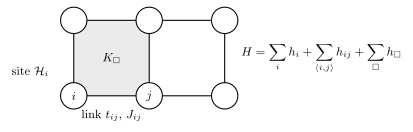
A lattice model is assembled from local data at several supports. A site carries $\mathcal H_i$, a link can carry hopping $t_{ij}$ or exchange $J_{ij}$, and a plaquette can carry a multi-site term $K_\square$.

Local Hilbert Spaces

For distinguishable site degrees of freedom with local spaces $\mathcal H_i$, the global space is

$$\mathcal H = \bigotimes_{i=1}^{L} \mathcal H_i.$$

If every site has dimension $q$, then

$$\dim\mathcal H = q^L.$$

This exponential growth is present even when the Hamiltonian contains only order-$L$ local terms. Scaling of Hilbert Space develops the counting and computational consequences.

The tensor-product form needs qualifications for identical particles. Bosonic and fermionic lattice modes live naturally in Fock space. After choosing an ordering, finite fermionic Fock space is isomorphic as a vector space to a product of local occupation spaces, but the operator algebra retains fermion-parity signs.

Spin and Qudit Sites

A spin-$s$ site has

$$\mathcal H_i \simeq \mathbb C^{2s+1}.$$

For spin $1/2$,

$$\mathcal H_i \simeq \mathbb C^2,$$

with Pauli operators or dimensionless spin operators $\mathbf s_i=\boldsymbol\sigma_i/2$.

A qudit model generalizes this to any finite local dimension $q$. The local basis may represent literal atomic levels, encoded qubits, clock variables, constrained charge states, or a truncated low-energy multiplet.

Finite local dimension makes operator norms and locality bounds particularly transparent, but it does not make the many-body spectrum easy.

Bosonic Sites

One ideal bosonic mode per site has local basis

$$\lvert0\rangle_i, \lvert1\rangle_i, \lvert2\rangle_i, \ldots,$$

so the exact local Hilbert space is infinite-dimensional. A numerical cutoff

$$0\le n_i\le n_{\max}$$

produces local dimension $n_{\max}+1$, but it changes the canonical commutator at the cutoff boundary. Convergence requires checking the probability weight near $n_{\max}$.

Hard-core bosons instead impose the physical or effective constraint

$$n_i\in\{0,1\}.$$

Their local state count matches spin $1/2$, although the identification of operators, symmetries, and exchange statistics must still be stated.

Fermionic Sites

One spinless fermionic mode has local states

$$\lvert0\rangle_i, \qquad \lvert1\rangle_i.$$

One spin-$1/2$ orbital has four states,

$$\lvert0\rangle_i, \quad \lvert\uparrow\rangle_i, \quad \lvert\downarrow\rangle_i, \quad \lvert\uparrow\downarrow\rangle_i.$$

Local occupancy is finite because of Pauli exclusion. Fermionic transfer operators nevertheless depend on a global mode ordering in an occupation basis. Spatially neighboring sites need not be adjacent in that ordering.

The practical sign conventions are developed in Fermionic Operators in Many-Body Models.

Constrained Local Spaces

Some models retain only a subspace of an underlying local Fock space. Examples include:

• no-double-occupancy states in a $t$–$J$ description;
• one dimer touching each vertex in a quantum dimer model;
• fixed electric-flux or Gauss-law sectors in lattice gauge models;
• Rydberg blockade constraints;
• fixed total spin in a projected atomic multiplet.

If $P$ projects onto the allowed space, a projected operator is

$$\widetilde O = POP.$$

In general,

$$\widetilde{AB} \ne \widetilde A\,\widetilde B,$$

because the intermediate state in $AB$ may leave the retained subspace. Constraints therefore alter operator algebra as well as state counting.

Operator Support

An operator $O_X$ is supported on a set of sites $X$ if it acts as the identity outside $X$:

$$O_X = O_X^{(X)} \otimes I_{X^{\mathrm c}}.$$

For fermionic systems, strictly local observable algebras are most naturally built from parity-even operators. Odd fermion operators on disjoint regions anticommute rather than commute, even though physical even observables can satisfy the expected locality structure.

Support identifies where an operation acts. Range identifies the diameter of that support in the graph metric.

Local Hamiltonians

A general lattice Hamiltonian can be organized as

$$H = \sum_{X\subseteq\Lambda} h_X,$$

where $h_X$ is supported on a finite subset $X$ of the lattice $\Lambda$.

For a finite-range Hamiltonian, there is a range $R$ such that

$$h_X=0 \qquad \text{when} \qquad \operatorname{diam}(X)>R.$$

For a short-range Hamiltonian, terms may extend farther but their norms decay sufficiently rapidly with diameter or separation.

Local does not mean noninteracting, weak, classical, or exactly solvable. It is a statement about operator support and geometry.

Geometric Locality Versus k-Locality

In quantum information, a Hamiltonian is called $k$-local when every term acts on at most $k$ subsystems. A two-site term connecting opposite ends of a large graph is $2$-local but not geometrically short-ranged.

Thus

$$|X|\le k$$

does not imply

$$\operatorname{diam}(X)\le R.$$

The distinction matters for Lieb–Robinson bounds, tensor networks, finite-size effects, and physical realizability.

Extensivity and Stability

For bounded local terms on a graph of bounded coordination, a finite-range Hamiltonian typically has order-$L$ terms. If

$$\lVert h_X\rVert \le J$$

and each site participates in at most a bounded number of terms, then

$$\lVert H\rVert \le \sum_X \lVert h_X\rVert = O(L).$$

This upper bound supports an extensive energy scale. It does not prove a particular thermodynamic phase or guarantee that every state has energy proportional to $L$.

Long-range interactions require more care. For pair couplings $J_{ij}$, a useful stability condition is a uniform bound of the form

$$\sup_i \sum_{j\ne i} |J_{ij}| < \infty$$

along the chosen sequence of larger systems. All-to-all models often need size-dependent normalization to retain a finite energy per site.

Locality and Information Propagation

Local lattice Hamiltonians do not impose relativistic microcausality, but they can limit how quickly initially separated observables develop a large commutator. Schematically,

$$\lVert[A_X(t),B_Y]\rVert \lesssim e^{-\mu[d(X,Y)-v|t|]}.$$

The constants and even the shape of the effective causal region depend on interaction range and decay. The precise theorem, assumptions, and limitations live in the Lieb–Robinson Bound reference entry.

This effective light cone helps explain why spatial locality remains useful despite an exponentially large Hilbert space.

Onsite Terms

An onsite Hamiltonian has the form

$$H_{\mathrm{site}} = \sum_i h_i.$$

Examples include:

$$\sum_i\epsilon_i n_i, \qquad -\sum_i\mathbf h_i\boldsymbol\cdot\mathbf s_i, \qquad \frac U2\sum_i n_i(n_i-1).$$

Onsite terms can set local energy splittings, chemical potentials, fields, anisotropies, constraints, or interactions between different modes at one site.

Calling a term onsite does not make it one-body. The bosonic operator $n_i(n_i-1)$ and the fermionic operator $n_{i\uparrow}n_{i\downarrow}$ are two-body interactions localized at one site.

Hopping Terms

A number-conserving hopping Hamiltonian is

$$H_t = -\sum_{i,j} \sum_{\alpha,\beta} t_{i\alpha,j\beta} c_{i\alpha}^\dagger c_{j\beta}.$$

Hermiticity requires

$$t_{i\alpha,j\beta} = t_{j\beta,i\alpha}^*.$$

The minus sign is conventional and can be absorbed into $t$ if definitions are adjusted consistently. On a graph, nonzero $t_{ij}$ defines directed or undirected transfer edges. Complex phases can encode magnetic flux or synthetic gauge fields.

Hopping changes local occupations while preserving total number:

$$\widehat N = \sum_{i,\alpha} n_{i\alpha}, \qquad [H_t,\widehat N]=0.$$

Quadratic Does Not Mean Single Particle

A quadratic hopping Hamiltonian acts on every particle-number sector of Fock space. It is noninteracting in the sense that its many-particle spectrum is assembled from one-particle modes, but it can still describe arbitrarily many bosons or fermions.

Diagonalizing the one-body matrix gives

$$H_t = \sum_\lambda \varepsilon_\lambda d_\lambda^\dagger d_\lambda.$$

Particle statistics then control how these one-particle energies are occupied. The dedicated tight-binding page develops translation-invariant dispersions, Fourier diagonalization, and the connection to bands.

Density Interactions

A general density interaction is

$$H_V = \frac12 \sum_{i,j} V_{ij} {:}n_i n_j{:}_0.$$

For separated sites, a common nearest-neighbor form is

$$H_V = V \sum_{\langle i,j\rangle} n_i n_j.$$

Density interactions are diagonal in the site-occupation basis. They do not directly move particles, although they change the energies and dynamics of configurations through their competition with hopping.

Long-range $V_{ij}$ can represent Coulomb, dipolar, cavity-mediated, or phenomenological interactions. Boundary and summation conventions must accompany slowly decaying kernels.

Exchange Interactions

A general bilinear spin interaction is

$$H_J = \sum_{\langle i,j\rangle} \sum_{a,b} J_{ij}^{ab} s_i^a s_j^b.$$

Special choices include:

• Ising exchange with only $J^{zz}$;
• XXZ exchange with $J^{xx}=J^{yy}\ne J^{zz}$;
• isotropic Heisenberg exchange with $J^{ab}=J\delta_{ab}$;
• antisymmetric Dzyaloshinskii–Moriya exchange;
• bond-dependent compass or Kitaev-type exchange.

The sign convention must be declared. In the common Heisenberg convention $H=J\sum\mathbf s_i\cdot\mathbf s_j$, positive $J$ favors antiferromagnetic alignment and negative $J$ favors ferromagnetic alignment.

Pairing and Conversion Terms

Not every lattice Hamiltonian conserves particle number. Pairing terms have the form

$$H_\Delta = \sum_{i,j} \left( \Delta_{ij}c_i^\dagger c_j^\dagger + \Delta_{ij}^*c_j c_i \right).$$

They change particle number by two while often preserving fermion parity. Bosonic models can include coherent conversion between species, pair hopping, or source terms.

The conserved quantities must be derived from the full Hamiltonian rather than inferred from a familiar model name.

Multi-Site and Ring Terms

Effective Hamiltonians can contain terms supported on three or more sites. A schematic four-site ring exchange is

$$H_K = K \sum_\square \left( P_\square + P_\square^{-1} \right),$$

where $P_\square$ cyclically permutes states around a plaquette.

Such terms can arise from higher-order virtual processes. They are local if each plaquette has bounded size, even though they are not pairwise.

Discarding multi-site terms is an approximation, not a consequence of locality.

Particle Models

Particle lattice models have creation and annihilation operators, occupation numbers, and often a global U(1) symmetry. Typical observables include:

• density and filling;
• compressibility;
• momentum distribution;
• one-particle spectral functions;
• superfluid stiffness or charge transport;
• double occupancy and pair correlations.

Examples include tight-binding, Hubbard, Bose–Hubbard, spinless-fermion, Anderson impurity, and Kondo-lattice descriptions.

The site labels refer to one-particle modes, not distinguishable particles.

Spin Models

Spin models assign a fixed local multiplet to each site. Their elementary operators rotate or compare local spin states rather than create or destroy microscopic particles.

Typical observables include:

• magnetization;
• spin correlations and structure factors;
• spin gaps;
• susceptibility;
• chirality and multipolar order;
• entanglement and string order.

Examples include Ising, XY, XXZ, Heisenberg, compass, and quantum-link models.

A spin flip can behave as a mobile quasiparticle in a suitable background, but that does not turn the microscopic spin model into a literal conserved-particle model.

Spin and Particle Models Are Related but Distinct

A spin-$1/2$ site and a hard-core boson site both have two local states. One can identify

$$b_i^\dagger \longleftrightarrow s_i^+, \qquad n_i \longleftrightarrow s_i^z+\frac12.$$

For hard-core bosons on different sites, these local operator algebras match a spin model. The mapping translates hopping into XY exchange and density interactions into Ising exchange plus lower-rank terms.

Spinless fermions also have two local states, but mapping them to spins in one dimension requires the parity strings and boundary-sector care derived in Jordan–Wigner Transformation. Equal local dimensions do not imply identical exchange statistics.

Effective Spin Models from Particle Models

At strong coupling, virtual particle motion can generate spin exchange within a low-energy subspace. For the repulsive half-filled Hubbard model,

$$J \sim \frac{4t^2}{U}$$

at leading order under standard assumptions.

This is a controlled effective relation in the regime $t/U\ll1$, not an operator identity between the full Hubbard and Heisenberg Hilbert spaces. Charge fluctuations are projected out, and higher-order terms remain.

The derivation and error structure belong to Effective Hamiltonians in Many-Body Systems.

Symmetries of Lattice Models

Symmetries can act on internal states, spatial labels, or both. Common examples include:

• global particle-number U(1);
• fermion parity;
• spin rotations or discrete spin flips;
• lattice translations and point-group operations;
• time reversal;
• particle-hole or sublattice transformations;
• gauge redundancies and Gauss-law constraints;
• subsystem symmetries acting on lines or planes.

A symmetry must preserve the graph, boundary conditions, coefficients, and constraints. A uniform bulk formula can lose translation or point-group symmetry on a finite open sample.

Onsite and Spatial Symmetries

An onsite internal symmetry factors as

$$U(g) = \bigotimes_i u_i(g).$$

A spatial symmetry instead permutes sites and may also rotate internal orbitals:

$$U_g c_{i\alpha}U_g^\dagger = \sum_\beta [D_g]_{\beta\alpha} c_{g(i),\beta}.$$

Nonsymmorphic and magnetic space-group structures require additional translations, phases, or antiunitary actions. This overview uses only the distinction needed to read generic lattice Hamiltonians.

Boundary Conditions Are Model Data

Open boundaries omit couplings beyond an edge. Periodic boundaries identify opposite edges and add wraparound bonds. Twisted boundaries insert a net phase around a periodic direction.

These choices affect:

• exact spatial symmetries;
• allowed momentum sectors;
• edge and surface states;
• finite-size gaps and degeneracies;
• fermion-parity sectors under nonlocal mappings;
• topological flux sectors.

Boundary effects can vanish in some bulk thermodynamic observables, but that is a conclusion to establish, not permission to omit the finite-system definition.

Energy Scales and Dimensionless Ratios

Most lattice physics depends on ratios of energy scales rather than isolated coefficients. Examples include

$$\frac Ut, \qquad \frac Jt, \qquad \frac hJ, \qquad \frac{k_{\mathrm B}T}{t}.$$

One overall nonzero energy scale can set units, but signs, phases, anisotropies, filling, geometry, and boundary conditions remain physical.

Parameter conventions vary. A Hamiltonian written with $-t$ hopping, $+J$ exchange, or dimensionful versus dimensionless spins must be translated before numerical values are compared.

Simple Formulas, Noncommuting Terms

Many canonical models have the structure

$$H = H_A+H_B,$$

where each part is separately simple but

$$[H_A,H_B] \ne 0.$$

In the Hubbard model, hopping is simple in momentum space and onsite repulsion is simple in real space. In the transverse-field Ising model, Ising exchange is diagonal in the $z$ basis while the transverse field is diagonal in the $x$ basis.

Competing noncommuting tendencies prevent simultaneous minimization and generate entanglement, collective behavior, and phase transitions.

Exact Limits and Benchmarks

Every model page should identify limits where the answer simplifies. Typical examples are:

• zero hopping or zero interaction;
• zero field or dominant field;
• a single site, bond, dimer, or plaquette;
• noninteracting particles;
• fully polarized spin states;
• high temperature;
• large coupling ratios with controlled projection.

Exact limits check signs, constants, degeneracies, and operator conventions. They do not establish the behavior at intermediate coupling.

Representative Model Families

Model family	Local degrees of freedom	Characteristic terms	Central competition
tight binding	bosonic or fermionic orbitals	hopping, onsite energy	geometry versus delocalization
transverse-field Ising	spin $1/2$	Ising exchange, transverse field	order versus quantum fluctuations
Heisenberg and XXZ	fixed spins	exchange, anisotropy, field	alignment, frustration, dimensionality
Hubbard	spinful fermions	hopping, onsite interaction	itinerancy versus local correlation
Bose–Hubbard	bosons	hopping, onsite pair repulsion	phase coherence versus number localization
spinless fermion chain	one fermion mode per site	hopping, density interaction	transport versus charge order
t–J	constrained spinful carriers	projected hopping, exchange	doped motion versus spin background
Kondo family	local spins plus itinerant fermions	exchange, hopping	screening versus magnetic correlations
Anderson impurity	localized and bath orbitals	hybridization, onsite interaction	charge fluctuation versus local moment

The table classifies ingredients, not full phase diagrams. Dimension, filling, coupling sign, range, and symmetry can change the physics within each family.

Why Lattice Models Can Be Universal

A model is a universal low-energy description when long-distance observables become insensitive to many microscopic details after relevant parameters and symmetries are matched.

The logic is not that every microscopic difference is unimportant. Rather, coarse graining can make some operators irrelevant while retaining:

• dimensionality and locality;
• symmetry and its possible anomalies;
• conserved quantities;
• low-energy degrees of freedom;
• topology and filling constraints;
• relevant and marginal couplings.

Different materials or platforms can then share critical exponents, scaling functions, collective modes, or effective Hamiltonians without sharing atomic details.

Projection and Scale Separation

Suppose the microscopic Hilbert space splits into a low-energy subspace $P$ and its complement $Q=I-P$. A schematic effective Hamiltonian is

$$H_{\mathrm{eff}} = PHP + O\!\left( \frac{V^2}{\Delta} \right),$$

where $V$ mixes the sectors and $\Delta$ is a separation scale.

Controlled use requires more than writing the ratio. One must identify the retained states, estimate omitted terms, transform observables, and state the energy or time window of validity.

Projection can generate longer-range, multi-site, and symmetry-allowed terms absent from the simplest named model.

Renormalization-Group View

Renormalization Group Preview owns the general construction of coarse-graining maps and coupling-space flows. For a lattice Hamiltonian, coarse graining generally generates every operator allowed by the retained symmetries and degrees of freedom. A simple effective model is stable only when omitted operators are irrelevant, parametrically small, forbidden, or explicitly included in an uncertainty budget.

Near a continuous transition, the correlation length can satisfy

$$\xi \gg a,$$

where $a$ is the microscopic lattice spacing. Long-distance behavior can then approach a continuum field theory even though the microscopic Hamiltonian is discrete.

Emergent rotational, Lorentz-like, or internal symmetry is possible, but it must be demonstrated in the low-energy limit. The lattice Hamiltonian does not possess that larger symmetry microscopically.

Lattice as Physical Model or Regulator

A physical lattice model can represent localized orbitals in a material or optical potential. Its spacing, coordination, and retained bands are part of the physics.

A regulator lattice approximates a continuum theory and is intended to approach

$$a\to0$$

with parameters matched appropriately. The Real-Space Representation gives this normalization and coupling dictionary.

These roles can overlap, but they should not be conflated. A fixed-spacing Hubbard model is not automatically a discretization destined for a continuum limit.

Filling and Sector Data

For particle models on $L$ sites, filling is commonly

$$\nu = \frac NL$$

or number per unit cell when several orbitals are present. Spin-resolved fillings may also be required.

The same Hamiltonian at different filling can realize qualitatively different regimes. Half filling, integer boson filling, dilute density, and a single impurity are distinct model specifications.

Canonical calculations fix conserved particle numbers. Grand-canonical calculations include

$$K = H-\mu N.$$

The chemical potential convention must be included when comparing phase boundaries or local energies.

Geometry and Frustration

Geometry affects more than coordination number. Odd cycles, non-bipartite graphs, and competing couplings can prevent every local interaction from being simultaneously minimized.

For antiferromagnetic Ising variables on a triangle, each bond favors opposite signs, but no configuration satisfies all three bonds. This is geometric frustration.

Quantum frustration also arises from noncommuting local terms even on simple geometries. The word should be tied to a specified inability to minimize compatible local tendencies, not used as a synonym for difficulty.

Observables and Diagnostics

A lattice model is not characterized by its ground-state energy alone. Common diagnostics include:

• local occupations, moments, and double occupancy;
• connected two-point functions;
• static and dynamic structure factors;
• gaps and finite-size level flow;
• response coefficients and stiffnesses;
• entanglement entropy and spectra;
• order parameters and Binder-type ratios;
• spectral functions and quasiparticle residues;
• transport and current correlations.

Each observable needs an operator definition and normalization. A phase label without diagnostics is not a reproducible result.

Phases Need Large-System Evidence

At finite size, the spectrum is discrete and exact symmetry eigenstates need not display a nonzero symmetry-breaking order parameter. Evidence for a phase can involve:

• correlation functions approaching long-range order;
• gaps that remain open or close with size;
• quasi-degenerate low-energy sectors;
• scaling collapse near a critical point;
• stiffness or topological response;
• entanglement and boundary signatures.

The Thermodynamic Limit explains why finite-size crossover and true bulk singularity must be distinguished.

Numerical Representation

Local Hamiltonians are often sparse in a local occupation or spin basis. Each basis vector connects only to configurations changed by one of the local terms.

This supports:

• sparse exact diagonalization in symmetry sectors;
• Krylov time evolution;
• matrix-product states and density-matrix renormalization in one dimension;
• tensor-network methods in higher dimensions;
• quantum Monte Carlo for sign-compatible models;
• cluster, embedding, and impurity approaches;
• analog or digital quantum simulation.

The global problem remains exponentially large, and each method has a regime of reliability. Sparse Matrices owns storage and matrix-vector details.

Symmetry Blocks and Basis Ordering

Before diagonalization, identify commuting charges such as

$$[H,Q_a]=0.$$

Working in fixed $Q_a$ sectors reduces memory and exposes exact degeneracies. Common sectors include total particle number, spin projection, crystal momentum, reflection parity, and fermion parity.

For fermions, declare the global mode ordering used to construct occupation basis states. A change of ordering is a unitary convention change when implemented consistently, but partial sign changes produce a different matrix.

Model-Building Workflow

1. Identify the physical regime and target observables.
2. Choose sites, links, orbitals, or constrained variables and define their local spaces.
3. Specify graph geometry, orientation, and boundaries.
4. List exact symmetries and conserved quantities.
5. Write every retained term with counting and sign conventions.
6. Explain the microscopic projection, discretization, or phenomenological rationale.
7. Estimate omitted terms and the energy window of validity.
8. Identify exact limits and the smallest nontrivial finite clusters.
9. Choose diagnostics before assigning phase labels.
10. Test finite-size, truncation, and parameter convergence.

Validation Checks

A lattice Hamiltonian should pass at least:

$$H^\dagger = H,$$

and every claimed conservation law should satisfy

$$[H,Q]=0.$$

Also check:

• each unoriented bond is counted once or compensated by a factor $1/2$;
• local and global Hilbert-space dimensions match the constraints;
• coefficient units and overall energy offsets are documented;
• open, periodic, and twisted matrices differ exactly where intended;
• one-site and two-site spectra match hand calculations;
• known noninteracting, atomic, strong-field, or strong-coupling limits are recovered;
• numerical results respect exact symmetries to solver tolerance;
• omitted local occupation or range truncations are converged.

Common Mistakes

• Treating the lattice drawing as a complete model specification.
• Confusing graph vertices with distinguishable particles.
• Assuming equal local dimensions imply identical bosonic, fermionic, and spin algebras.
• Calling every two-site Hamiltonian geometrically local.
• Calling every onsite term one-body.
• Counting both bond orientations without adjusting coefficients.
• Forgetting Hermitian-conjugate hopping or pairing terms.
• Comparing hopping or exchange signs across incompatible conventions.
• Ignoring filling, chemical potential, and conserved sector.
• Assuming open boundaries merely remove irrelevant edge details.
• Treating a named model as a quantitatively complete material description.
• Dropping symmetry-allowed terms without a scale estimate.
• Presenting a strong-coupling effective model outside its validity regime.
• Inferring a bulk phase from one small cluster without scaling diagnostics.
• Assuming locality makes the model exactly solvable or numerically easy.
• Confusing a physical lattice with a continuum regulator.

Quick Reference

Question	Required model data
What lives locally?	site, link, or cell Hilbert space and constraints
What is the geometry?	graph, embedding, distances, orientation, boundaries
What is local?	support and range of every term
What moves particles?	hopping or conversion operators
What correlates sites?	density, exchange, pairing, or multi-site interactions
What is conserved?	charges derived from commutators with the full Hamiltonian
What sets the regime?	dimensionless coupling ratios, filling, temperature, size
Why is the model valid?	projection, discretization, symmetry, or phenomenological argument
How is it tested?	exact limits, small clusters, convergence, and observables

Summary

A quantum lattice model is a structured tuple of local spaces, graph data, operators, coefficients, constraints, symmetries, and boundaries. Its short Hamiltonian is meaningful only together with those definitions.

Locality organizes the Hamiltonian as

$$H = \sum_X h_X,$$

while hopping, interactions, exchange, and fields encode distinct physical processes. Particle and spin models can map into one another in controlled settings, but equal state counts do not erase statistics or constraints.

Simple lattice models become universal when they retain the low-energy degrees of freedom, symmetries, locality, topology, and relevant couplings of a wider microscopic class. That claim requires scale separation, matched observables, and a stated validity regime.

Exercises

Exercise 1: Compare local and global dimensions

Find the full Hilbert-space dimension for $L$ sites in each case:

1. spin $1/2$;
2. one spinful fermionic orbital per site;
3. one bosonic mode truncated to $0\le n_i\le n_{\max}$.

Solution

A spin-$1/2$ site has two states, so

$$\dim\mathcal H_{\mathrm{spin}} = 2^L.$$

A spinful fermionic orbital has the four states empty, up, down, and doubly occupied, so

$$\dim\mathcal F_{\mathrm{fermion}} = 4^L.$$

A bosonic site with occupations $0$ through $n_{\max}$ has $n_{\max}+1$ states, so

$$\dim\mathcal H_{\mathrm{boson,cut}} = (n_{\max}+1)^L.$$

The bosonic result describes the truncated numerical space, not the exact unbounded local Fock space.

Exercise 2: Hermiticity of hopping

Consider

$$H_t = -\sum_{i,j} t_{ij}c_i^\dagger c_j.$$

Derive the condition on $t_{ij}$ for $H_t$ to be Hermitian.

Solution

Taking the adjoint gives

$$H_t^\dagger = -\sum_{i,j} t_{ij}^*c_j^\dagger c_i.$$

Relabel $i\leftrightarrow j$:

$$H_t^\dagger = -\sum_{i,j} t_{ji}^*c_i^\dagger c_j.$$

Therefore $H_t^\dagger=H_t$ when

$$t_{ij} = t_{ji}^*.$$

The hopping matrix must be Hermitian. A complex phase on one orientation must be conjugated on the reverse orientation.

Exercise 3: Total number under hopping and density interactions

Let

$$N = \sum_i n_i,$$

and consider

$$H = -\sum_{i,j}t_{ij}c_i^\dagger c_j + \frac12\sum_{i,j}V_{ij}n_i n_j.$$

Show that $[H,N]=0$ for bosons or fermions.

Solution

The number operator satisfies

$$[N,c_i^\dagger] = c_i^\dagger, \qquad [N,c_j] = -c_j.$$

Hence

$$\begin{aligned} [N,c_i^\dagger c_j] &= [N,c_i^\dagger]c_j + c_i^\dagger[N,c_j] \\ &= c_i^\dagger c_j - c_i^\dagger c_j =0. \end{aligned}$$

Every $n_i$ commutes with total number, so every product $n_i n_j$ also commutes with it. Therefore $[N,H]=0$, equivalently $[H,N]=0$.

Exercise 4: Extensivity bound for a bond Hamiltonian

Let a graph have $L$ sites and maximum degree $z$. Suppose

$$H = \sum_{(i,j)\in E} h_{ij}, \qquad \lVert h_{ij}\rVert\le J.$$

Show that $\lVert H\rVert\le JzL/2$.

Solution

The triangle inequality gives

$$\lVert H\rVert \le \sum_{(i,j)\in E} \lVert h_{ij}\rVert \le J|E|.$$

The handshaking identity is

$$2|E| = \sum_i z_i.$$

Since every degree obeys $z_i\le z$,

$$|E| \le \frac{zL}{2}.$$

Combining the bounds yields

$$\lVert H\rVert \le \frac{JzL}{2}.$$

Bounded coordination and bounded bond strength therefore produce an operator-norm upper bound linear in system size.

Exercise 5: Hard-core bosons and spin one-half

On each site identify

$$\lvert0\rangle \longleftrightarrow \lvert\downarrow\rangle, \qquad \lvert1\rangle \longleftrightarrow \lvert\uparrow\rangle.$$

Show that $b_i^\dagger\leftrightarrow s_i^+$ and $n_i\leftrightarrow s_i^z+1/2$. Translate nearest-neighbor boson hopping into spin operators.

Solution

On the two-state local space,

$$b_i^\dagger\lvert0\rangle_i = \lvert1\rangle_i, \qquad b_i^\dagger\lvert1\rangle_i = 0,$$

which is the action of $s_i^+$ under the stated identification. Also,

$$s_i^z+\frac12$$

has eigenvalues $0$ on $\lvert\downarrow\rangle$ and $1$ on $\lvert\uparrow\rangle$, so it equals $n_i$.

The hopping term becomes

$$\begin{aligned} -t\sum_{\langle i,j\rangle} (b_i^\dagger b_j+b_j^\dagger b_i) &= -t\sum_{\langle i,j\rangle} (s_i^+s_j^-+s_j^+s_i^-) \\ &= -2t\sum_{\langle i,j\rangle} (s_i^x s_j^x+s_i^y s_j^y). \end{aligned}$$

This local mapping applies to hard-core bosons. Mapping spinless fermions requires additional parity strings in one dimension.

Exercise 6: Competing terms in a two-spin Ising dimer

For

$$H = -J\sigma_1^z\sigma_2^z - h(\sigma_1^x+\sigma_2^x),$$

identify the ground states in the limits $h=0$ with $J>0$, and $J=0$ with $h>0$. Explain why the two terms compete.

Solution

At $h=0$ and $J>0$, the exchange energy is minimized by aligned $z$ spins:

$$\lvert\uparrow\uparrow\rangle, \qquad \lvert\downarrow\downarrow\rangle.$$

They are degenerate with energy $-J$.

At $J=0$ and $h>0$, each site minimizes $-h\sigma^x$ in the $+1$ eigenstate of $\sigma^x$. The ground state is

$$\lvert+\rangle_x \otimes \lvert+\rangle_x.$$

The operators $\sigma^z$ and $\sigma^x$ do not commute. A state sharp in the exchange-preferred $z$ basis is not sharp in the field-preferred $x$ basis, so the two terms cannot generally be minimized simultaneously.

Exercise 7: Bond counting on a periodic chain

How many distinct nearest-neighbor bonds does a chain of $L\ge3$ sites have with open boundaries and with periodic boundaries? What error results from summing both orientations without a compensating factor?

Solution

An open chain has bonds

$$(1,2),(2,3),\ldots,(L-1,L),$$

for a total of $L-1$.

A periodic chain adds $(L,1)$, giving $L$ distinct unoriented bonds.

If one sums both $(i,j)$ and $(j,i)$ for a symmetric bond operator, each physical bond appears twice. Without a factor $1/2$ or a directed-term convention, the interaction energy is doubled.

Exercise 8: Classify an all-to-all model

Consider an all-to-all Ising interaction

$$H_L = -J_L \sum_{1\le i<j\le L} \sigma_i^z\sigma_j^z.$$

Classify the Hamiltonian by interaction arity and geometric range. What scaling of $J_L$ keeps the fully polarized energy of order $L$, and which properties does that normalization fail to restore?

Solution

Each term acts on two sites, so the Hamiltonian is two-local in arity, but it is geometrically all-to-all. Since the pair count is quadratic, $J_L\propto 1/L$ keeps the aligned energy of order $L$. The normalization controls the leading energy scale; it does not make the interaction short-ranged or additive. Extensive and Intensive Quantities owns the derivation and Kac-scaling audit.

References

1. A. Auerbach, Interacting Electrons and Quantum Magnetism, Springer (1994).
2. P. Coleman, Introduction to Many-Body Physics, Cambridge University Press (2015).
3. A. Altland and B. Simons, Condensed Matter Field Theory, 2nd ed., Cambridge University Press (2010).
4. S. Sachdev, Quantum Phase Transitions, 2nd ed., Cambridge University Press (2011).
5. T. Giamarchi, Quantum Physics in One Dimension, Oxford University Press (2004).
6. P. Fazekas, Lecture Notes on Electron Correlation and Magnetism, World Scientific (1999).
7. E. Fradkin, Field Theories of Condensed Matter Physics, 2nd ed., Cambridge University Press (2013).
8. X.-G. Wen, Quantum Field Theory of Many-Body Systems, Oxford University Press (2004).
9. M. Lewenstein, A. Sanpera, and V. Ahufinger, Ultracold Atoms in Optical Lattices, Oxford University Press (2012).
10. E. H. Lieb and D. W. Robinson, “The finite group velocity of quantum spin systems,” Communications in Mathematical Physics 28, 251–257 (1972).