Tight-Binding Model

The tight-binding model describes coherent motion among a retained set of localized orbitals. Instead of resolving the continuous wavefunction between neighboring orbital centers, it records that motion through Hamiltonian matrix elements called hopping amplitudes. Translation-invariant hopping turns localized site states into extended crystal-momentum eigenstates and, on a periodic chain, produces the characteristic cosine dispersion.

The basic model is quadratic: it contains onsite one-body energies and hopping, but no particle–particle interaction. It can therefore be solved by diagonalizing a one-particle Hermitian matrix. The same matrix may describe one particle, many noninteracting fermions, or many noninteracting bosons; statistics and filling determine how its modes are occupied.

Canonical Scope

This page is the canonical home for:

• the generic hopping Hamiltonian on a finite graph in one-particle and Fock-space language;
• nearest-neighbor hopping and its sign conventions;
• exact diagonalization on arbitrary finite graphs;
• Fourier diagonalization of translation-invariant chains;
• cosine dispersions, bandwidth, velocity, and effective mass;
• open, periodic, and twisted boundary conditions for the basic chain;
• the algebraic extension to longer-range and multi-orbital quadratic models;
• the occupation of one-particle modes by noninteracting fermions or bosons;
• validity checks and the limits of what a noninteracting hopping model can establish.

The Tight-Binding Chain dossier owns the convention-complete one-dimensional baseline and finite validation targets. The Tight-Binding Dimer owns the two-site first encounter. Momentum-Space Representation owns Fourier normalization, Brillouin-zone kinematics, and interaction vertices. Tight-Binding Models is the canonical quantum-matter method page for continuum projection, crystalline orbital embeddings, material Bloch matrices, spin–orbit terms, Wannier downfolding, and the worked SSH, square, and honeycomb models.

Optical Lattices owns the AMO construction, recoil scales, loading, and calibration that connect a standing-wave potential to measured hopping parameters. Detailed electronic structure, material-specific orbital choices, band topology, and realistic crystal modeling belong in Tight-Binding Models and its neighboring Quantum Matter articles. The present page develops the generic lattice Hamiltonian that those subjects use.

Physical Idea

Choose normalized localized states

$$\lvert i,\alpha\rangle,$$

where $i$ labels a site or unit cell and $\alpha$ labels an orbital, sublattice, spin, or another internal mode. A particle initially localized near one site can evolve into neighboring orbitals because the Hamiltonian has off-diagonal matrix elements.

For one orbital per site, a useful schematic form is

$$h_{\mathrm{tb}} = \sum_i \epsilon_i \lvert i\rangle\langle i\rvert - \sum_{i\ne j} t_{ij} \lvert i\rangle\langle j\rvert.$$

The onsite energy $\epsilon_i$ is diagonal in the localized basis. The hopping $t_{ij}$ couples distinct orbitals. Hopping is coherent unitary coupling, not an irreversible stochastic jump.

Localized Orbitals from a Continuum Problem

Suppose a one-particle continuum Hamiltonian $\widehat h$ is projected onto orthonormal localized orbitals $w_{i\alpha}(\mathbf r)$. Its retained matrix elements are

$$h_{i\alpha,j\beta} = \int d^dr\, w_{i\alpha}^*(\mathbf r) \widehat h w_{j\beta}(\mathbf r).$$

The projected Hamiltonian is

$$h_{\mathrm{proj}} = \sum_{i,\alpha} \sum_{j,\beta} h_{i\alpha,j\beta} \lvert i,\alpha\rangle \langle j,\beta\rvert.$$

A common sign convention defines off-diagonal hopping by

$$t_{i\alpha,j\beta} = -h_{i\alpha,j\beta}, \qquad (i,\alpha)\ne(j,\beta).$$

The minus sign is conventional. A trustworthy calculation states whether $t_{ij}$ denotes the matrix element itself or its negative.

Projection and Truncation

Tight binding is not defined solely by drawing a lattice. It is an approximation or effective model only after specifying:

• which localized orbitals are retained;
• how well separated they are from omitted orbitals;
• which hopping ranges are kept;
• whether overlap between basis functions has been orthogonalized;
• whether interactions, spin–orbit terms, or external fields are omitted or added;
• which observables and energy window the model is intended to reproduce.

Exponential localization often makes distant hopping amplitudes small, but it does not make every nearest-neighbor truncation exact. Symmetry can also force a nominally short-range matrix element to vanish while a longer-range one remains important.

Nonorthogonal Basis Caveat

Atomic-orbital trial functions are not always orthogonal. If

$$S_{ab} = \langle a\vert b\rangle \ne \delta_{ab},$$

then the coefficients obey a generalized eigenvalue problem,

$$\sum_b h_{ab}u_b = E \sum_b S_{ab}u_b.$$

Replacing $S$ by the identity without an orthogonalization or a controlled small-overlap argument changes the model. The canonical tight-binding formulas below assume an orthonormal retained basis.

One-Particle Hamiltonian

Compress the combined label $(i,\alpha)$ into $a$. The most general finite tight-binding Hamiltonian is a Hermitian matrix,

$$h_{\mathrm{tb}} = \sum_{a,b} h_{ab} \lvert a\rangle\langle b\rvert, \qquad h_{ba}=h_{ab}^*.$$

Separating onsite and intersite terms gives

$$h_{\mathrm{tb}} = \sum_a \epsilon_a \lvert a\rangle\langle a\rvert - \sum_{a\ne b} t_{ab} \lvert a\rangle\langle b\rvert,$$

with

$$\epsilon_a\in\mathbb R, \qquad t_{ba}=t_{ab}^*.$$

If each unordered bond is counted once, write instead

$$\begin{aligned} h_{\mathrm{tb}} ={}& \sum_a \epsilon_a \lvert a\rangle\langle a\rvert \\ &- \sum_{\langle a,b\rangle} \left( t_{ab} \lvert a\rangle\langle b\rvert + t_{ab}^* \lvert b\rangle\langle a\rvert \right). \end{aligned}$$

These two conventions are equivalent only when their summation rules are respected.

Hermiticity and Bond Orientation

A directed hopping amplitude has an orientation:

$$t_{ab} \quad \text{multiplies} \quad \lvert a\rangle\langle b\rvert.$$

Hermiticity fixes the reverse process to have amplitude $t_{ab}^*$. For real hopping, both directions carry the same real coefficient. For complex hopping, the phase changes sign under reversal.

A frequent factor-of-two error comes from summing both ordered pairs $(a,b)$ and $(b,a)$ and also appending a Hermitian conjugate. Use either an ordered-pair sum or an unordered-bond sum, not both.

Graph Interpretation

For one orbital on each vertex of a graph, uniform real nearest-neighbor hopping gives

$$h_{\mathrm{tb}} = \epsilon_0 I-tA,$$

where $A$ is the graph adjacency matrix:

$$A_{ij} = \begin{cases} 1,&i\text{ and }j\text{ are connected},\\ 0,&\text{otherwise}. \end{cases}$$

The graph spectrum of $A$ therefore determines the one-particle tight-binding spectrum. Geometry enters through connectivity, loops, boundaries, coordination, and any spatial dependence assigned to the amplitudes.

Adjacency Matrix Versus Discrete Laplacian

The graph Laplacian is

$$L = D-A,$$

where $D_{ii}=z_i$ is the degree of vertex $i$. On a regular graph with degree $z$,

$$tL = tzI-tA.$$

Thus a Laplacian kinetic term and a nearest-neighbor tight-binding term differ only by the constant onsite shift $tz$ on a regular graph. On an irregular graph or at an open boundary, $D$ is not generally proportional to the identity, so replacing $-tA$ by $tL$ changes boundary onsite terms and can change the spectrum.

The continuum-discretization meaning of this distinction is developed in Real-Space Representation.

Second-Quantized Hamiltonian

Introduce a creation operator $c_a^\dagger$ for each retained orbital. The Fock-space lift of the one-particle matrix is

$$H_{\mathrm{tb}} = \sum_{a,b} h_{ab} c_a^\dagger c_b.$$

For onsite energies and unordered hopping bonds,

$$\begin{aligned} H_{\mathrm{tb}} ={}& \sum_a \epsilon_a n_a \\ &- \sum_{\langle a,b\rangle} \left( t_{ab}c_a^\dagger c_b + t_{ab}^*c_b^\dagger c_a \right), \end{aligned}$$

where

$$n_a=c_a^\dagger c_a.$$

The operators may be bosonic or fermionic. Their algebra changes allowed occupations and many-body states, but it does not change the one-particle matrix $h$.

Quadratic Does Not Mean One Particle

The Hamiltonian is quadratic because every term contains one creation and one annihilation operator. It acts on every particle-number sector. A quadratic Hamiltonian can therefore describe a macroscopic noninteracting gas, not merely a single particle.

What is absent is a term such as

$$U \sum_i n_{i\uparrow}n_{i\downarrow},$$

or another quartic interaction. Adding that term for spinful fermions produces the Hubbard Model, whose competition between hopping and interaction is no longer solved by a one-particle basis change. Projecting out doublons in its strong-repulsion sector instead leads to the constrained t–J Model Preview. Coupling the band locally to a separate spin gives the Kondo Model Preview. For bosons, hopping plus onsite pair interaction produces the Bose–Hubbard Model.

Number Conservation

The total number operator is

$$\widehat N = \sum_a n_a.$$

Every hopping term destroys one particle in one mode and creates one in another, so

$$[H_{\mathrm{tb}},\widehat N] = 0.$$

Hopping redistributes particles without changing their total number. Pairing terms such as $c_a^\dagger c_b^\dagger+\mathrm{h.c.}$ are quadratic but are not part of the number-conserving tight-binding model defined here.

Exact Diagonalization on an Arbitrary Graph

Solve the one-particle eigenproblem

$$\sum_b h_{ab}u_{b\nu} = \varepsilon_\nu u_{a\nu}.$$

Choose the eigenvectors orthonormally:

$$\sum_a u_{a\nu}^*u_{a\mu} = \delta_{\nu\mu}.$$

Define normal-mode operators

$$d_\nu = \sum_a u_{a\nu}^*c_a, \qquad c_a = \sum_\nu u_{a\nu}d_\nu.$$

The transformation preserves the canonical commutation or anticommutation relations. Substitution gives

$$H_{\mathrm{tb}} = \sum_\nu \varepsilon_\nu d_\nu^\dagger d_\nu.$$

This is the complete solution of the number-conserving quadratic model on a finite graph.

Many-Body Spectrum

In the normal-mode occupation basis,

$$\lvert\{n_\nu\}\rangle,$$

the energy is

$$E_{\{n_\nu\}} = \sum_\nu \varepsilon_\nu n_\nu.$$

For spinless fermions,

$$n_\nu\in\{0,1\},$$

while for ordinary bosons,

$$n_\nu\in\{0,1,2,\ldots\}.$$

Adding a nearest-neighbor density interaction to a one-dimensional spinless hopping band gives the Spinless Fermion Chains $t$–$V$ model. That interaction changes the problem from a one-body band-filling exercise into an interacting Luttinger-liquid and charge-order problem.

If spin or another conserved flavor is present, each flavor has its own mode occupation. The one-body eigenvalues are shared when the hopping is flavor independent.

The Nearest-Neighbor Chain

Take $N$ sites at

$$x_j=ja, \qquad j=0,\ldots,N-1,$$

with lattice spacing $a$, uniform onsite energy $\epsilon_0$, and real nearest-neighbor hopping $t$. The standard Hamiltonian is

$$\begin{aligned} H ={}& \epsilon_0 \sum_j n_j \\ &- t \sum_j \left( c_{j+1}^\dagger c_j + c_j^\dagger c_{j+1} \right). \end{aligned}$$

The meaning of the final bond depends on the boundary condition. This small piece of model data changes the finite-size eigenstates.

Periodic Boundary Conditions

For a ring,

$$c_{j+N}=c_j.$$

There are $N$ bonds, including the bond from $N-1$ back to $0$. Translation by one site is an exact symmetry.

The allowed wave numbers satisfy

$$e^{ikNa}=1,$$

so

$$k_m = \frac{2\pi m}{Na}.$$

Choose any $N$ inequivalent representatives modulo $2\pi/a$. A common first Brillouin zone is

$$-\frac{\pi}{a} \le k < \frac{\pi}{a}.$$

The endpoints differ by a reciprocal-lattice vector and are not distinct.

Lattice Fourier Modes

Use the unitary transform

$$c_j = \frac1{\sqrt N} \sum_k e^{ikx_j}c_k,$$

with inverse

$$c_k = \frac1{\sqrt N} \sum_j e^{-ikx_j}c_j.$$

Discrete orthogonality gives

$$\frac1N \sum_{j=0}^{N-1} e^{i(k-q)x_j} = \delta_{kq}.$$

Consequently,

$$\sum_j n_j = \sum_k n_k.$$

The transform changes basis; it does not change the number of one-particle modes.

Fourier Diagonalization

For the forward hopping sum,

$$\sum_j c_{j+1}^\dagger c_j = \sum_k e^{-ika} c_k^\dagger c_k.$$

The reverse hopping gives the complex conjugate phase:

$$\sum_j c_j^\dagger c_{j+1} = \sum_k e^{ika} c_k^\dagger c_k.$$

Therefore

$$H = \sum_k \varepsilon(k) c_k^\dagger c_k,$$

with

$$\varepsilon(k) = \epsilon_0 - t \left( e^{ika}+e^{-ika} \right).$$

Using $e^{ix}+e^{-ix}=2\cos x$,

$$\varepsilon(k) = \epsilon_0-2t\cos(ka).$$

The localized site basis and the energy basis are different whenever $t\ne0$.

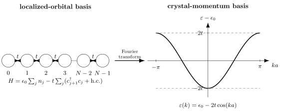
A periodic nearest-neighbor chain is diagonalized by the lattice Fourier transform. Real uniform hopping produces one cosine band with edges $\epsilon_0\mp2t$ for $t>0$.

Dispersion Relation

The function $\varepsilon(k)$ is periodic:

$$\varepsilon \left( k+\frac{2\pi}{a} \right) = \varepsilon(k).$$

This periodicity reflects crystal-momentum equivalence, not repeated physically distinct states. A finite ring samples the dispersion at $N$ allowed $k$ values; the continuous curve is the large-$N$ interpolation.

For real hopping, the dispersion is even:

$$\varepsilon(-k) = \varepsilon(k).$$

That equality follows from the combination of real hopping and inversion-symmetric nearest-neighbor geometry.

Band Edges and Bandwidth

For $t>0$,

$$\varepsilon_{\min} = \epsilon_0-2t \quad \text{at} \quad k=0,$$

and

$$\varepsilon_{\max} = \epsilon_0+2t \quad \text{at} \quad k=\frac{\pi}{a}.$$

The bandwidth is

$$W = \varepsilon_{\max} - \varepsilon_{\min} = 4t.$$

For arbitrary real $t$,

$$W=4\lvert t\rvert.$$

The onsite energy shifts the whole band but does not change its width.

Group Velocity

For a wave packet narrow in crystal momentum, the semiclassical group velocity is

$$v(k) = \frac1{\hbar} \frac{d\varepsilon}{dk} = \frac{2ta}{\hbar} \sin(ka).$$

Thus

$$\lvert v(k)\rvert \le \frac{2\lvert t\rvert a}{\hbar}.$$

At a band extremum, the group velocity vanishes even though the eigenstate is spatially extended. Localization and zero group velocity are different statements.

Effective Mass Near a Band Edge

For $t>0$ and $\lvert ka\rvert\ll1$,

$$\cos(ka) = 1-\frac{(ka)^2}{2} + O((ka)^4).$$

The band bottom is therefore

$$\varepsilon(k) = \epsilon_0-2t + ta^2k^2 + O(k^4a^4).$$

Comparing with

$$\varepsilon(k) = \varepsilon_{\min} + \frac{\hbar^2k^2}{2m^*} +\cdots$$

gives

$$m^* = \frac{\hbar^2}{2ta^2}.$$

At the top of the same band, the curvature is negative and the electron effective mass defined by curvature is negative. Hole variables reorganize nearly filled-band dynamics with a positive hole mass. The compact curvature formula is collected in Effective Mass.

Density of States Preview

The density of states counts one-particle modes per energy interval. In one dimension,

$$g(E) \propto \sum_{k_*} \frac1{ \left| d\varepsilon/dk \right|_{k_*} },$$

where the sum runs over solutions of $\varepsilon(k_*)=E$. The group velocity vanishes at the cosine-band edges, so the one-dimensional density of states has band-edge singularities in the infinite-chain limit.

Normalization conventions and dimensional examples belong to Density of States.

Open Boundary Conditions

For an open chain, sites are labeled

$$j=1,\ldots,N,$$

and the hopping sum contains only

$$j=1,\ldots,N-1.$$

There is no bond between sites $N$ and $1$. Translation by one site is not an exact symmetry, so periodic plane waves are not exact finite-chain eigenstates.

The one-particle difference equation in the interior is

$$E\psi_j = \epsilon_0\psi_j - t \left( \psi_{j-1}+\psi_{j+1} \right).$$

Open ends are encoded by

$$\psi_0=0, \qquad \psi_{N+1}=0.$$

These are endpoint conditions for the discrete recurrence, not extra physical sites.

Standing-Wave Eigenstates

The normalized open-chain eigenvectors are

$$\psi_m(j) = \sqrt{\frac{2}{N+1}} \sin(q_mj),$$

where

$$q_m = \frac{\pi m}{N+1}, \qquad m=1,\ldots,N.$$

Their energies are

$$E_m = \epsilon_0-2t\cos q_m.$$

The variable $q_m$ is dimensionless. A wave number may be defined as $k_m=q_m/a$, but it is not an eigenvalue of an exact finite-chain translation symmetry.

The open chain has $N$ standing-wave modes, exactly matching its $N$ sites.

Boundary Effects

Open and periodic chains approach the same bulk dispersion as $N\to\infty$, but their finite spectra are not identical. Open boundaries:

• remove one bond relative to a ring;
• break discrete translation symmetry;
• replace traveling waves by standing waves;
• permit boundary-localized states when edge couplings or onsite terms are modified;
• change finite-size level spacing and degeneracies.

Boundary Conditions on Lattices owns systematic finite-size comparisons, momentum-sector bookkeeping, and fermion-parity caveats. Here the boundary conditions are developed only far enough to solve the basic hopping chain.

Twisted Boundary Conditions

A twist $\theta$ imposes

$$c_{j+N} = e^{i\theta}c_j.$$

Allowed plane waves satisfy

$$e^{ikNa} = e^{i\theta},$$

so

$$k_m(\theta) = \frac{2\pi m+\theta}{Na}.$$

The energies are

$$\varepsilon_m(\theta) = \epsilon_0 - 2t \cos \left( \frac{2\pi m+\theta}{N} \right).$$

A twist shifts the finite momentum grid through the same bulk dispersion. Because $\theta$ and $\theta+2\pi$ describe the same boundary condition,

$$\operatorname{Spec}H(\theta+2\pi) = \operatorname{Spec}H(\theta)$$

as an unordered set, although individual level labels can permute.

Boundary Phase and Flux

The twist can be placed on the boundary bond,

$$-t \left( e^{-i\theta}c_0^\dagger c_{N-1} + e^{i\theta}c_{N-1}^\dagger c_0 \right),$$

or distributed uniformly over all bonds by a site-dependent phase redefinition. The spectrum depends on the total loop phase, not on where a particular gauge places it.

For a charged particle on a ring, this total phase can represent an Aharonov–Bohm flux. The gauge principle and its limits are developed in Peierls Phase Preview.

Boundary Comparison

Boundary	Final bond	Exact one-site translation	Natural modes
open	absent	no	standing waves
periodic	real hopping	yes	discrete plane waves
twisted	phase $e^{i\theta}$	gauge-dependent representation of a twisted translation	shifted plane waves

All three require exactly $N$ one-particle eigenstates for $N$ single-orbital sites.

Sign of the Hopping

On an open nearest-neighbor chain, the transformation

$$c_j \longmapsto (-1)^j c_j$$

changes

$$t\longmapsto -t.$$

It exchanges the apparent band minimum and maximum by shifting momentum by $\pi/a$. On a bipartite graph with hopping only between the two sublattices, the same sign change can be made with opposite phases on the two sublattices.

This does not mean that every hopping sign is unphysical. On an odd ring, a uniform sign flip changes the phase accumulated around the loop. With several hopping ranges or frustrated loops, no single site rephasing need remove all relative signs.

Local Basis Phases

Under a rephasing

$$c_i' = e^{i\chi_i}c_i,$$

the hopping coefficients in the primed basis are

$$t_{ij}' = e^{i(\chi_i-\chi_j)} t_{ij}.$$

Individual link phases therefore depend on the localized-orbital convention. Around a closed oriented loop $C$, the phase

$$\Phi_C = \arg \prod_{(ij)\in C} t_{ij}$$

is invariant under site rephasings. Spectra can depend on such loop phases.

Real Hopping and Time Reversal

For a spinless model written in a basis where every hopping and onsite energy is real, complex conjugation $K$ satisfies

$$KhK^{-1}=h.$$

This is the standard spinless time-reversal symmetry. A loop phase not congruent to $0$ or $\pi$ modulo $2\pi$ generally obstructs a globally real representation and can break this symmetry. A $\pi$ loop phase can still be represented by real signed hoppings.

For spinful particles, time reversal also acts on spin and squares to $-1$ for a single spin-$1/2$ particle. Spin-dependent hopping then requires a matrix treatment beyond the scalar real-hopping criterion.

Hypercubic Lattices

On a $d$-dimensional hypercubic lattice with primitive spacings $a_\mu$ and real axis-dependent hoppings $t_\mu$,

$$\varepsilon(\mathbf k) = \epsilon_0 - 2 \sum_{\mu=1}^d t_\mu \cos(k_\mu a_\mu).$$

For isotropic $t_\mu=t>0$,

$$\varepsilon_{\min} = \epsilon_0-2dt,$$

and

$$\varepsilon_{\max} = \epsilon_0+2dt.$$

The bandwidth is

$$W=4d\lvert t\rvert.$$

Coordination and bandwidth are related for this simple lattice, but the exact bandwidth of a general graph is not determined by coordination alone.

General Translation-Invariant Hopping

Let $\boldsymbol\delta$ run over directed displacement vectors and let

$$t(-\boldsymbol\delta) = t(\boldsymbol\delta)^*.$$

Then

$$H = - \sum_{j,\boldsymbol\delta} t(\boldsymbol\delta) c_{j+\boldsymbol\delta}^\dagger c_j$$

has dispersion

$$\varepsilon(\mathbf k) = - \sum_{\boldsymbol\delta} t(\boldsymbol\delta) e^{-i\mathbf k\cdot\boldsymbol\delta},$$

up to any separately displayed onsite energy. Hermiticity makes $\varepsilon(\mathbf k)$ real.

This compact formula is useful, but its bond-counting convention must be stated: the displacement set here includes both directions.

Longer-Range Hopping

For a one-dimensional inversion-symmetric chain with real hopping $t_r$ across $r$ lattice spacings,

$$\varepsilon(k) = \epsilon_0 - 2 \sum_{r\ge1} t_r\cos(rka).$$

Nearest-neighbor tight binding retains only $t_1$. A next-nearest-neighbor term adds

$$-2t_2\cos(2ka).$$

It can shift band extrema, change curvature, break the simple bipartite spectral symmetry, and alter the density of states. A fit that needs substantial $t_2$ is still tight binding, but it is not a nearest-neighbor model.

Several Orbitals per Unit Cell

Let $\alpha=1,\ldots,M$ label orbitals or sublattices within each cell. Translation symmetry block-diagonalizes the Hamiltonian as

$$H = \sum_{\mathbf k} \mathbf c_{\mathbf k}^\dagger h(\mathbf k) \mathbf c_{\mathbf k},$$

where

$$\mathbf c_{\mathbf k} = \begin{pmatrix} c_{\mathbf k1}\\ \vdots\\ c_{\mathbf kM} \end{pmatrix},$$

and $h(\mathbf k)$ is an $M\times M$ Hermitian matrix.

Fourier transformation resolves translation sectors. A second, generally $\mathbf k$-dependent unitary transformation diagonalizes $h(\mathbf k)$ inside each sector.

Two-Orbital Bloch Matrix

A generic two-orbital block is

$$h(k) = \begin{pmatrix} \epsilon_A(k) & f(k)\\ f(k)^* & \epsilon_B(k) \end{pmatrix}.$$

Its two band energies are

$$\begin{aligned} E_\pm(k) ={}& \frac{ \epsilon_A(k)+\epsilon_B(k) }{2} \\ &\pm \sqrt{ \left[ \frac{ \epsilon_A(k)-\epsilon_B(k) }{2} \right]^2 + \lvert f(k)\rvert^2 }. \end{aligned}$$

Hybridization $f(k)$ generally splits levels that would cross in its absence. Symmetry may force $f(k)$ to vanish at selected momenta, in which case crossings can remain.

The SSH Model and Graphene Dirac Model are compact examples of multi-sublattice hopping, but their topology and material interpretation have separate canonical homes.

Relation to Bloch Theory

For a periodic lattice, the localized operators and crystal-momentum operators are related by a discrete Fourier transform. Translation by a lattice vector acts diagonally on $c_{\mathbf k}^\dagger\lvert0\rangle$, so each $\mathbf k$ labels a translation character.

With one orbital per primitive cell and no additional internal mixing, there is one band per retained flavor:

$$\mathbf k \longmapsto \varepsilon(\mathbf k).$$

With $M$ orbitals per cell, diagonalizing $h(\mathbf k)$ yields $M$ bands:

$$h(\mathbf k) u_n(\mathbf k) = \varepsilon_n(\mathbf k) u_n(\mathbf k).$$

This is the tight-binding route to band structure. Bloch theorem is the symmetry statement; tight binding is a particular localized-basis representation and truncation of the Hamiltonian.

Wannier and Bloch Descriptions

In an isolated set of bands, localized orbitals and extended Bloch states can be related by Fourier transformation. Wannier Functions owns the exact Bloch-frame construction, localization, disentanglement, and topology diagnostics; this page begins with declared lattice orbitals and hopping matrices and owns their graph and Fock-space consequences. The same retained subspace can therefore have:

• a real-space description with localized orbitals and hopping amplitudes;
• a momentum-space description with band energies and orbital eigenvectors.

These are complementary bases, not competing physical theories. Within a fixed selected subspace the complete basis transform is exact; selecting or disentangling that subspace and truncating the resulting hopping matrix are separate approximations.

Tight Binding Versus Nearly Free Particles

Tight binding begins from localized orbitals and treats intersite hybridization through hopping. A nearly-free-particle expansion begins from plane waves and treats a periodic potential as coupling reciprocal-space modes.

Both can describe the same periodic Hamiltonian in different regimes. Neither slogan alone guarantees quantitative accuracy. The useful basis is the one in which the retained subspace is small and omitted couplings are controlled.

Filling and Statistics

The dispersion does not determine a many-body state until statistics and filling are specified. For noninteracting fermions at zero temperature, the ground state fills the lowest available one-particle modes up to the particle number. For noninteracting bosons, repeated occupation of the lowest mode is allowed.

In a grand-canonical description,

$$K = H-\mu\widehat N = \sum_\nu \left( \varepsilon_\nu-\mu \right) d_\nu^\dagger d_\nu.$$

The chemical potential changes occupations; it does not alter the eigenvectors of a number-conserving one-body Hamiltonian.

Calling a tight-binding model metallic, insulating, magnetic, or superconducting requires more than displaying $\varepsilon(k)$. One must specify filling, degeneracies, gaps to other bands, interactions, disorder, dimension, and the observable criterion.

Spin and Flavor

If hopping is independent of a flavor $\sigma$,

$$H = \sum_{\mathbf k,\sigma} \varepsilon(\mathbf k) c_{\mathbf k\sigma}^\dagger c_{\mathbf k\sigma}.$$

Each one-particle energy is flavor degenerate. Spin-independent hopping alone does not produce magnetism. Magnetism requires a state-selection mechanism such as interactions, spin-dependent fields, exchange, or explicit spin-dependent hopping.

Disorder and Inhomogeneity

An onsite potential

$$H_V = \sum_j V_j n_j$$

or position-dependent hopping $t_{ij}$ breaks translation symmetry unless its pattern is periodic. The model remains quadratic and exactly reducible to a one-particle matrix, but ordinary Fourier modes no longer diagonalize it.

Real-space eigenvectors, inverse participation ratios, local densities, and boundary sensitivity then become useful. Disorder-induced localization is a deeper subject; a localized finite-size eigenvector by itself does not establish a thermodynamic localization transition.

Sublattice Symmetry

Consider a bipartite graph with only hopping between sublattices $A$ and $B$ and no onsite term after subtracting a common $\epsilon_0$. Define

$$\Gamma = \begin{cases} +1,&A,\\ -1,&B. \end{cases}$$

As a one-particle operator,

$$\{\Gamma,h-\epsilon_0 I\} = 0.$$

If $(h-\epsilon_0 I)\lvert u\rangle=E\lvert u\rangle$, then

$$(h-\epsilon_0 I) \Gamma\lvert u\rangle = -E \Gamma\lvert u\rangle.$$

The spectrum is symmetric about $\epsilon_0$. Same-sublattice hopping or nonuniform onsite energies generally break this symmetry.

Translation and Inversion

Translation symmetry requires hopping and onsite data to repeat from cell to cell. In a one-orbital Bravais lattice,

$$t_{ij} = t(\mathbf R_i-\mathbf R_j).$$

Inversion symmetry imposes an additional relation between displacement amplitudes. For scalar real hopping,

$$t(\boldsymbol\delta) = t(-\boldsymbol\delta)$$

implies

$$\varepsilon(\mathbf k) = \varepsilon(-\mathbf k).$$

With internal orbitals, inversion can exchange sublattices and must be represented by a matrix; evenness of each matrix element is not the correct general criterion.

Observables

Useful one-body observables include:

• site occupations $\langle n_i\rangle$;
• momentum occupations $\langle n_{\mathbf k}\rangle$ when translation labels apply;
• bond correlations $\langle c_i^\dagger c_j\rangle$;
• wave-packet center and spreading;
• density of states and local density of states;
• response to a boundary twist;
• orbital weights in multi-band eigenvectors.

The continuity equation and bond-current conventions are developed in Density Operators and Current Operators. A current must be derived from the stated hopping orientation and charge convention rather than guessed from a diagram.

Continuum Limit Near a Band Minimum

For the nearest-neighbor chain,

$$\varepsilon(k)-\varepsilon_{\min} = 2t \left[ 1-\cos(ka) \right].$$

Using

$$1-\cos(ka) = \frac{(ka)^2}{2} + O((ka)^4),$$

one obtains

$$\varepsilon(k)-\varepsilon_{\min} = ta^2k^2 + O(k^4a^4).$$

To approximate a continuum particle of mass $m$, choose

$$t = \frac{\hbar^2}{2ma^2},$$

and subtract the divergent energy offset associated with the band minimum as $a\to0$. Merely sending $a\to0$ at fixed $t$ does not preserve a fixed continuum mass.

Physical Lattice Versus Numerical Grid

For a physical lattice, $a$ is an atomic, molecular, optical, or synthetic spacing and need not be taken to zero. The band is a physical low-energy structure.

For a numerical grid, the lattice is a regulator. Then $a\to0$ is a refinement limit, hopping must scale with $a$, and boundary terms must reproduce the intended continuum operator. The Real-Space Representation owns that continuum–lattice dictionary.

Exact Limits and Checks

Several limits expose mistakes quickly.

Atomic limit

At $t=0$,

$$H = \epsilon_0 \sum_j n_j.$$

Every site orbital has the same one-particle energy $\epsilon_0$ in the uniform model.

Dimer limit

For two sites with one bond,

$$h = \begin{pmatrix} \epsilon_0&-t\\ -t&\epsilon_0 \end{pmatrix},$$

with energies

$$\epsilon_0-t, \qquad \epsilon_0+t.$$

This is the Tight-Binding Dimer. A two-site periodic-chain sum needs special bond-counting care because the left and right neighbor coincide.

Trace check

For any finite matrix,

$$\sum_\nu\varepsilon_\nu = \operatorname{Tr}h.$$

If all onsite energies equal $\epsilon_0$ and hopping has no diagonal part,

$$\sum_\nu\varepsilon_\nu = N\epsilon_0.$$

The hopping redistributes one-particle energies around their mean but does not change the trace.

Mode-count check

One orbital on each of $N$ sites gives exactly $N$ one-particle eigenvalues, including multiplicities. A Fourier transform, boundary twist, or basis rotation cannot change this count.

Numerical Representation

For short-range hopping, the one-particle matrix is sparse. In one dimension with open boundaries it is tridiagonal; on a finite-dimensional local lattice, the number of nonzero entries grows linearly with the number of sites at fixed coordination.

Useful computational choices include:

• dense diagonalization for small systems and all eigenvectors;
• sparse extremal eigensolvers for band edges or selected states;
• Fourier diagonalization for exact translation invariance;
• Krylov propagation for wave-packet dynamics;
• shift-invert methods for interior eigenvalues;
• twisted-boundary sampling for finite-size momentum resolution.

Sparse storage and conditioning live in Sparse Matrices. Exploiting translation symmetry is exact only when the finite Hamiltonian and boundary condition possess that symmetry.

Modeling Workflow

For a new tight-binding problem:

1. define the retained localized orbitals and their normalization;
2. specify the graph, unit cell, and boundary condition;
3. state the sign and bond-counting convention;
4. list onsite, hopping, flavor, and phase data;
5. identify exact symmetries and conserved sectors;
6. decide whether one-particle, fermionic, or bosonic Fock space is intended;
7. diagonalize in real space or translation sectors as appropriate;
8. test exact limits, trace, mode count, and boundary dependence;
9. compare against the energy window or observables the model is meant to reproduce;
10. add interactions only with a separate physical justification.

Common Mistakes

• Calling hopping an incoherent random jump.
• Omitting the boundary condition from a finite-chain Hamiltonian.
• Counting each bond twice while also adding its Hermitian conjugate.
• Mixing $t_{ij}=-h_{ij}$ with a convention in which $t_{ij}=h_{ij}$.
• Treating crystal momentum as unrestricted mechanical momentum.
• Forgetting that an open chain has standing waves, not exact plane-wave eigenstates.
• Assuming the sign of every hopping can be removed on any graph.
• Using a nonorthogonal orbital basis as though its overlap matrix were the identity.
• Calling a quadratic tight-binding Hamiltonian interacting because it acts on many particles.
• Inferring a metal, insulator, magnet, or superconductor without specifying filling and missing physics.
• Taking a continuum limit at fixed $t$ instead of scaling $t$ with $a^{-2}$ when appropriate.
• Treating a finite-size boundary state or level crossing as a bulk phase diagnosis.

Quick Reference

Item	Formula or statement
finite model	$H=\sum_{ab}h_{ab}c_a^\dagger c_b$
Hermiticity	$h_{ba}=h_{ab}^*$
periodic chain	$\varepsilon(k)=\epsilon_0-2t\cos(ka)$
allowed periodic modes	$k_m=2\pi m/(Na)$
open-chain modes	$q_m=\pi m/(N+1)$
twisted modes	$k_m=(2\pi m+\theta)/(Na)$
one-dimensional bandwidth	$W=4\lvert t\rvert$
group velocity	$v(k)=\hbar^{-1}d\varepsilon/dk$
band-bottom mass	$m^*=\hbar^2/(2ta^2)$ for $t>0$
hypercubic dispersion	$\epsilon_0-2\sum_\mu t_\mu\cos(k_\mu a_\mu)$

Summary

The tight-binding model is a localized-basis representation of a one-body Hamiltonian. On a finite graph it is solved by diagonalizing a Hermitian hopping matrix. On a periodic lattice, translation symmetry organizes that diagonalization by crystal momentum; nearest-neighbor hopping on a chain gives a cosine band.

The simplicity is precise but limited. Boundary conditions select finite-size modes, basis phases redistribute link phases, longer-range hopping reshapes the dispersion, and multiple orbitals produce matrix-valued Bloch Hamiltonians. Statistics and filling determine the many-body occupation of the one-particle spectrum, while interactions require additional terms and new methods.

Exercises

Exercise 1: Fourier diagonalization of the ring

Starting from

$$H = \epsilon_0\sum_j n_j - t\sum_j \left( c_{j+1}^\dagger c_j + c_j^\dagger c_{j+1} \right),$$

with $c_{j+N}=c_j$, derive the diagonal momentum-space Hamiltonian.

Solution

Insert

$$c_j = \frac1{\sqrt N} \sum_k e^{ikja}c_k.$$

For the forward term,

$$\begin{aligned} \sum_j c_{j+1}^\dagger c_j ={}& \frac1N \sum_{j,k,q} e^{-ik(j+1)a} e^{iqja} c_k^\dagger c_q \\ ={}& \sum_k e^{-ika} c_k^\dagger c_k, \end{aligned}$$

where discrete orthogonality sets $q=k$. The reverse term gives $e^{ika}$. Hence

$$H = \sum_k \left[ \epsilon_0 - t(e^{ika}+e^{-ika}) \right] c_k^\dagger c_k.$$

Therefore

$$H = \sum_k \left[ \epsilon_0-2t\cos(ka) \right] c_k^\dagger c_k.$$

Exercise 2: Open-chain standing waves

Verify that

$$\psi_m(j) = \sqrt{\frac{2}{N+1}} \sin \left( \frac{\pi mj}{N+1} \right)$$

solves the open-chain eigenproblem, and find its energy.

Solution

Set

$$q_m = \frac{\pi m}{N+1}.$$

The endpoint conditions hold because

$$\sin(0)=0, \qquad \sin(q_m(N+1))=\sin(\pi m)=0.$$

Using

$$\sin(q(j-1)) + \sin(q(j+1)) = 2\cos q\sin(qj),$$

the difference equation gives

$$\begin{aligned} E_m\psi_m(j) ={}& \epsilon_0\psi_m(j) \\ &- 2t\cos(q_m)\psi_m(j). \end{aligned}$$

Thus

$$E_m = \epsilon_0-2t\cos q_m.$$

The displayed normalization follows from the discrete sine orthogonality relation.

Exercise 3: Twisted momentum grid

For $c_{j+N}=e^{i\theta}c_j$, derive the allowed $k$ values and show that the spectrum is $2\pi$-periodic in $\theta$ as a set.

Solution

A plane wave obeys

$$c_{j+N} \propto e^{ik(j+N)a} = e^{ikNa}e^{ikja}.$$

The boundary condition requires

$$e^{ikNa} = e^{i\theta}.$$

Therefore

$$k_m(\theta) = \frac{2\pi m+\theta}{Na}.$$

Increasing $\theta$ by $2\pi$ gives

$$k_m(\theta+2\pi) = k_{m+1}(\theta).$$

The labels are permuted, so the unordered set of energies is unchanged:

$$\operatorname{Spec}H(\theta+2\pi) = \operatorname{Spec}H(\theta).$$

Exercise 4: Effective mass and grid scaling

Expand the one-dimensional cosine band near $k=0$ for $t>0$. What scaling of $t$ reproduces a continuum mass $m$ as $a\to0$?

Solution

Near $k=0$,

$$\cos(ka) = 1-\frac{k^2a^2}{2} + O(k^4a^4).$$

Hence

$$\varepsilon(k) = \epsilon_0-2t + ta^2k^2 +\cdots.$$

Matching the energy above the minimum to

$$\frac{\hbar^2k^2}{2m}$$

requires

$$t = \frac{\hbar^2}{2ma^2}.$$

The band-bottom offset must also be subtracted or absorbed into the onsite energy. Holding $t$ fixed would send the effective mass to infinity as $a\to0$.

Exercise 5: Flipping the hopping sign

Show that $c_j\mapsto(-1)^jc_j$ flips the sign of nearest-neighbor hopping on an open chain. Why does the same argument fail on an odd periodic ring?

Solution

Each nearest-neighbor bilinear transforms as

$$c_{j+1}^\dagger c_j \longmapsto (-1)^{j+1} (-1)^j c_{j+1}^\dagger c_j = - c_{j+1}^\dagger c_j.$$

Thus every open-chain bond changes sign.

On a periodic ring, the boundary bond connects $N-1$ to $0$. Its sign factor is

$$(-1)^{N-1}(-1)^0.$$

For odd $N$, this factor is $+1$, whereas every ordinary nearest-neighbor bond has factor $-1$. One cannot flip all bonds consistently. Equivalently, an odd cycle is not bipartite, and the loop phase is invariant under site rephasings.

Exercise 6: Next-nearest-neighbor extrema

Consider

$$\varepsilon(k) = \epsilon_0 - 2t_1\cos(ka) - 2t_2\cos(2ka).$$

Find the stationary-point condition and identify when extrema away from $ka=0,\pi$ are possible.

Solution

Let $x=ka$. Differentiation gives

$$\frac{d\varepsilon}{dx} = 2t_1\sin x + 4t_2\sin(2x).$$

Using $\sin(2x)=2\sin x\cos x$,

$$\frac{d\varepsilon}{dx} = 2\sin x \left( t_1+4t_2\cos x \right).$$

The usual stationary points satisfy $\sin x=0$, so $x=0$ or $\pi$ modulo $2\pi$. Additional stationary points satisfy

$$\cos x = - \frac{t_1}{4t_2}.$$

Real solutions exist when

$$\left| \frac{t_1}{4t_2} \right| \le 1.$$

Thus sufficiently strong next-nearest-neighbor hopping can create extrema away from the center and edge of the Brillouin zone.

Exercise 7: Two-orbital bands

Diagonalize

$$h(k) = \begin{pmatrix} \Delta & f(k)\\ f(k)^*&-\Delta \end{pmatrix}.$$

When can the two bands touch?

Solution

The characteristic equation is

$$E^2 - \Delta^2 - \lvert f(k)\rvert^2 = 0.$$

Therefore

$$E_\pm(k) = \pm \sqrt{ \Delta^2+\lvert f(k)\rvert^2 }.$$

The bands touch only if the square root vanishes, requiring both

$$\Delta=0$$

and

$$f(k)=0$$

at the same momentum. A nonzero sublattice offset $\Delta$ opens a gap in this two-band model.

Exercise 8: Statistics and many-body counting

A finite tight-binding matrix has $M$ nondegenerate one-particle modes. How many fixed-$Q$ Fock states exist for spinless fermions and for one species of bosons? Write their energies.

Solution

For spinless fermions, each mode is occupied at most once. Choosing $Q$ occupied modes from $M$ gives

$$\dim\mathcal H_Q^{\mathrm F} = \binom{M}{Q}.$$

For bosons, distributing $Q$ identical particles among $M$ modes gives

$$\dim\mathcal H_Q^{\mathrm B} = \binom{M+Q-1}{Q}.$$

In either case, a mode-occupation configuration has energy

$$E_{\{n_\nu\}} = \sum_{\nu=1}^M \varepsilon_\nu n_\nu.$$

The difference lies in the allowed occupation numbers and therefore in which sums occur.

References

• N. W. Ashcroft and N. D. Mermin, Solid State Physics, Holt, Rinehart and Winston, 1976.
• C. Kittel, Introduction to Solid State Physics, 8th ed., Wiley, 2005.
• S. H. Simon, The Oxford Solid State Basics, Oxford University Press, 2013.
• M. P. Marder, Condensed Matter Physics, 2nd ed., Wiley, 2010.
• J. C. Slater and G. F. Koster, “Simplified LCAO Method for the Periodic Potential Problem”, Physical Review 94, 1498–1524, 1954.
• G. H. Wannier, “The Structure of Electronic Excitation Levels in Insulating Crystals”, Physical Review 52, 191–197, 1937.
• E. N. Economou, Green’s Functions in Quantum Physics, 3rd ed., Springer, 2006.
• A. Altland and B. Simons, Condensed Matter Field Theory, 2nd ed., Cambridge University Press, 2010.
• P. Fazekas, Lecture Notes on Electron Correlation and Magnetism, World Scientific, 1999.
• P. Coleman, Introduction to Many-Body Physics, Cambridge University Press, 2015.