Tight-Binding Chain

One-Sentence Description

The tight-binding chain is a quadratic one-dimensional lattice model in which coherent nearest-neighbor hopping turns one localized orbital per site into an exactly calculable cosine band.

This dossier fixes the model data needed to compare spectra and computations: Hilbert-space meaning, hopping sign, bond list, boundary condition, exact-solution scope, observables, limiting cases, and finite validation targets. The Tight-Binding Model teaching article owns the derivation from localized orbitals, Fourier diagonalization, generalized hopping graphs, and the broader connection to Bloch and Wannier descriptions.

Baseline Model Record

Unless a variant is stated explicitly, this dossier uses the following chain.

Field	Baseline choice
sites	$N$ sites at $x_j=ja$, with $j=0,\ldots,N-1$
retained basis	one orthonormal localized orbital $\lvert j\rangle$ per site
one-particle space	$\mathcal H_1\simeq\mathbb C^N$
Fock-space lift	one spinless bosonic or fermionic mode per site, stated explicitly
onsite energy	uniform real $\epsilon_0$
hopping	real nearest-neighbor amplitude $t>0$ in the convention $h_{j,j+1}=-t$
interactions	none
internal flavor	none
boundaries	open, periodic, or twisted, always stated
energy scale	$t$
lattice spacing	$a$
thermodynamic reference	periodic rings followed by $N\to\infty$ at fixed $a$

The one-particle problem does not require particle statistics. Statistics enter only when the same one-body matrix is lifted to a many-particle Fock space. Likewise, a band dispersion alone does not specify a many-body ground state: particle number or chemical potential, statistics, temperature, and any omitted internal degeneracy must also be supplied.

The baseline assumes an orthonormal retained basis. A nonorthogonal orbital set instead leads to a generalized eigenvalue problem $hu=ESu$ and is not silently identified with this model.

Degrees of Freedom and Hilbert Spaces

One-particle formulation

The localized basis obeys

$$\langle j\vert k\rangle = \delta_{jk}, \qquad \sum_{j=0}^{N-1} \lvert j\rangle\langle j\rvert = \mathbb I_{\mathcal H_1}.$$

A one-particle state is

$$\lvert\psi\rangle = \sum_{j=0}^{N-1} \psi_j\lvert j\rangle, \qquad \sum_j\lvert\psi_j\rvert^2 = 1.$$

The site amplitudes are basis coefficients, not classical probabilities moving by random jumps. Their coherent phases determine interference, current, and band formation.

Fock-space formulation

Introduce annihilation and creation operators $c_j$ and $c_j^\dagger$. For fermions,

$$\{c_j,c_k^\dagger\} = \delta_{jk}, \qquad \{c_j,c_k\} = 0,$$

whereas bosons obey

$$[c_j,c_k^\dagger] = \delta_{jk}, \qquad [c_j,c_k] = 0.$$

In either case,

$$n_j = c_j^\dagger c_j, \qquad \widehat N = \sum_j n_j.$$

For spinless fermions, $n_j\in\{0,1\}$ and the fixed-$Q$ sector has dimension

$$\dim\mathcal H_Q^{\mathrm F} = \binom NQ.$$

For one bosonic species, $n_j\in\mathbb N_0$ and

$$\dim\mathcal H_Q^{\mathrm B} = \binom{N+Q-1}{Q}.$$

The Fock-space Hamiltonian is many-particle in its domain but remains noninteracting because it is quadratic and number conserving.

Hamiltonian and Conventions

Open chain

For open boundaries, the one-particle operator is

$$\begin{aligned} h_{\mathrm O} ={}& \epsilon_0 \sum_{j=0}^{N-1} \lvert j\rangle\langle j\rvert \\ &- t \sum_{j=0}^{N-2} \left( \lvert j+1\rangle\langle j\rvert + \lvert j\rangle\langle j+1\rvert \right). \end{aligned}$$

There are $N-1$ undirected bonds. The corresponding Fock-space operator is

$$\begin{aligned} H_{\mathrm O} ={}& \epsilon_0 \sum_{j=0}^{N-1} n_j \\ &- t \sum_{j=0}^{N-2} \left( c_{j+1}^\dagger c_j + c_j^\dagger c_{j+1} \right). \end{aligned}$$

Periodic chain

For a ring, site labels are understood modulo $N$:

$$\lvert j+N\rangle = \lvert j\rangle, \qquad c_{j+N} = c_j.$$

The Hamiltonian is

$$\begin{aligned} H_{\mathrm P} ={}& \epsilon_0 \sum_{j=0}^{N-1} n_j \\ &- t \sum_{j=0}^{N-1} \left( c_{j+1}^\dagger c_j + c_j^\dagger c_{j+1} \right). \end{aligned}$$

An ordinary simple ring has $N$ distinct bonds for $N\ge3$. At $N=2$, the modular shorthand visits the same undirected pair twice. The two-site limit in this dossier therefore means one explicitly listed bond, as in the Tight-Binding Dimer.

Bond-list form

For either boundary condition, let $\mathcal B$ be the set of distinct undirected bonds. Then

$$H = \epsilon_0\widehat N - t \sum_{\{j,k\}\in\mathcal B} \left( c_j^\dagger c_k + c_k^\dagger c_j \right).$$

This form makes bond counting explicit and is the preferred starting point for finite numerics. If a directed sum already contains both orientations, adding a separate Hermitian-conjugate term would double the hopping.

Energy zero and hopping sign

In a fixed-$Q$ sector, the onsite term contributes the constant

$$\epsilon_0 Q.$$

It shifts every energy in that sector without changing eigenvectors or gaps. Across sectors, however, it changes particle-addition energies and cannot be dropped without also stating how the chemical potential is transformed.

On an open bipartite chain, the basis rephasing

$$c_j \longmapsto (-1)^j c_j$$

maps $t\mapsto-t$. The same transformation works on an even ring. It fails to flip every bond on an odd ring because the loop phase is invariant under local basis rephasings. Thus the baseline $t>0$ is harmless for an open chain or even ring, but hopping signs around general loops carry physical information.

Complete Problem Data

For a reproducible calculation, the Hamiltonian expression must be supplemented by:

• $N$, $a$, and the ordered site or bond list;
• open, periodic, or twisted boundaries;
• $\epsilon_0$, $t$, and the hopping-sign convention;
• one-particle, fermionic Fock, or bosonic Fock interpretation;
• fixed particle number $Q$ or ensemble data such as $\mu$ and $T$;
• the observable normalization and energy zero;
• any disorder, flavor, flux, longer-range hopping, or interaction term;
• the finite-size sequence used for a bulk inference.

Natural dimensionless variables include

$$\frac{E-\epsilon_0}{t}, \qquad ka, \qquad \nu=\frac QN, \qquad \frac{k_{\mathrm B}T}{t}, \qquad \theta,$$

where $\nu$ is a Fock-space filling and $\theta$ is a dimensionless boundary twist. The one-particle baseline has no nontrivial coupling ratio: after subtracting $\epsilon_0$ and measuring energy in units of $t$, only geometry and boundary data remain.

Symmetries and Conserved Quantities

Number conservation

The quadratic lift has a global $U(1)$ symmetry,

$$c_j \longmapsto e^{i\alpha}c_j,$$

and

$$[H,\widehat N] = 0.$$

Fixed-particle-number sectors are therefore exact invariant subspaces.

Translation

On a uniform periodic ring, one-site translation $T$ acts as

$$T c_j T^{-1} = c_{j+1}, \qquad T^N = \mathbb I,$$

and satisfies

$$[H_{\mathrm P},T] = 0.$$

The translation eigenvalues $e^{ika}$ label the $N$ crystal-momentum sectors. Open boundaries remove this exact symmetry even though the bulk couplings remain uniform.

Inversion and spinless time reversal

For a reflection-symmetric chain, inversion sends $j$ to its reflected site and commutes with $H$. With real onsite energies and hoppings, complex conjugation $K$ in the site basis gives the spinless time-reversal relation

$$K h K^{-1} = h.$$

For a ring carrying a generic twist, time reversal and reflection both reverse the loop phase:

$$\theta \longmapsto -\theta.$$

They are symmetries of the same twisted Hamiltonian only at twists equivalent to $0$ or $\pi$ modulo $2\pi$, although spectra at $\theta$ and $-\theta$ are related.

Sublattice spectral symmetry

An open chain and an even ring are bipartite. Define the one-particle sublattice operator

$$\Gamma\lvert j\rangle = (-1)^j\lvert j\rangle.$$

After subtracting the uniform onsite energy,

$$h' = h-\epsilon_0\mathbb I,$$

nearest-neighbor hopping obeys

$$\Gamma h'\Gamma^{-1} = -h'.$$

Consequently, every one-particle eigenvalue $\epsilon_0+\lambda$ is paired with $\epsilon_0-\lambda$. This is a one-particle chiral or sublattice spectral symmetry. It should not be promoted automatically to a many-body particle–hole statement without specifying statistics, filling, constants, and the transformation of the Fock operators.

Exact Solution Status

Finite one-particle problem

For any declared finite graph, the tight-binding problem is exactly the spectral problem of an $N\times N$ Hermitian matrix:

$$h u_\alpha = \varepsilon_\alpha u_\alpha.$$

A unitary eigenvector matrix $U$ gives

$$U^\dagger hU = \operatorname{diag} \left( \varepsilon_1,\ldots,\varepsilon_N \right).$$

“Exact” here means reduction to finite Hermitian diagonalization. Closed-form radicals are neither expected nor required for a generic large graph.

Quadratic many-particle lift

Define normal modes

$$d_\alpha = \sum_j U_{j\alpha}^*c_j.$$

The same unitary transformation preserves either the canonical anticommutation or commutation relations and yields

$$H = \sum_{\alpha=1}^{N} \varepsilon_\alpha d_\alpha^\dagger d_\alpha.$$

Every occupation configuration is an eigenstate with energy

$$E_{\{n_\alpha\}} = \sum_{\alpha=1}^{N} \varepsilon_\alpha n_\alpha.$$

For spinless fermions, $n_\alpha=0$ or $1$; for bosons, $n_\alpha$ is any nonnegative integer. This solves the number-conserving free many-body problem once the one-particle modes are known. Adding density interactions, pairing, a local constraint, or a dynamical gauge field changes the solution class.

Scope of the claim

The following statements are exact for the baseline:

• all finite one-particle eigenvalues and eigenvectors;
• all free Fock-space energies and occupation eigenstates;
• the periodic dispersion and open-chain standing waves;
• equilibrium occupation observables reducible to the one-body spectrum;
• unitary one-particle dynamics and free many-body Gaussian correlators.

The baseline does not establish an interacting phase diagram, quasiparticle lifetime, thermalization mechanism, Mott transition, superconductivity, or material-specific band accuracy.

Periodic Exact Fingerprints

Use the unitary Fourier transform

$$c_j = \frac1{\sqrt N} \sum_{m} e^{ik_mja} c_{k_m}, \qquad k_m = \frac{2\pi m}{Na},$$

where any $N$ inequivalent integer values of $m$ may be chosen. The Hamiltonian becomes

$$H_{\mathrm P} = \sum_m \varepsilon(k_m) c_{k_m}^\dagger c_{k_m},$$

with

$$\varepsilon(k) = \epsilon_0 - 2t\cos(ka).$$

The finite ring samples a periodic function:

$$\varepsilon \left( k+\frac{2\pi}{a} \right) = \varepsilon(k).$$

There are exactly $N$ inequivalent one-particle modes, not an infinite number of distinct copies of the band.

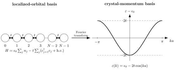
The periodic baseline is diagonal in crystal momentum. For $t>0$, the one-particle band runs from $\epsilon_0-2t$ at $k=0$ to $\epsilon_0+2t$ at the Brillouin-zone edge; a finite ring retains only its $N$ allowed momenta.

Band edges and velocity

For real nonzero $t$,

$$W = \varepsilon_{\max} - \varepsilon_{\min} = 4\lvert t\rvert.$$

For $t>0$,

$$\varepsilon_{\min} = \epsilon_0-2t, \qquad \varepsilon_{\max} = \epsilon_0+2t.$$

The wave-packet group velocity is

$$v(k) = \frac1{\hbar} \frac{d\varepsilon}{dk} = \frac{2ta}{\hbar} \sin(ka),$$

so

$$\lvert v(k)\rvert \le \frac{2\lvert t\rvert a}{\hbar}.$$

An extended eigenstate at a band edge has zero group velocity; zero velocity is not localization.

Effective mass

Near the $t>0$ band minimum,

$$\varepsilon(k) = \epsilon_0-2t + ta^2k^2 + O(k^4a^4).$$

Matching to $\hbar^2k^2/(2m^*)$ gives

$$m^* = \frac{\hbar^2}{2ta^2}.$$

The curvature at the band top has the opposite sign. Effective Mass owns the general tensor definition and convention checks.

Infinite-chain density of states

Per site and per retained flavor, the normalized one-particle density of states is

$$\rho(E) = \frac{ \Theta\!\left( 2\lvert t\rvert-\lvert E-\epsilon_0\rvert \right) }{ \pi \sqrt{ 4t^2-(E-\epsilon_0)^2 } }.$$

It satisfies

$$\int_{-\infty}^{\infty} \rho(E)\,dE = 1.$$

The inverse-square-root divergences at the two band edges are one-dimensional van Hove singularities, not delta-function bound states. Density of States owns normalization across dimensions and degeneracy conventions.

Open-Chain Exact Fingerprints

For $j=0,\ldots,N-1$, the normalized eigenvectors are

$$\psi_m(j) = \sqrt{\frac{2}{N+1}} \sin \left[ \frac{\pi m(j+1)}{N+1} \right],$$

with

$$m = 1,\ldots,N.$$

Their energies are

$$E_m = \epsilon_0 - 2t \cos \left( \frac{\pi m}{N+1} \right).$$

These are standing waves satisfying the discrete endpoint conditions

$$\psi(-1) = 0, \qquad \psi(N) = 0.$$

The dimensionless angle $\pi m/(N+1)$ is sometimes denoted $q_m$. It is not the eigenvalue of an exact finite-chain translation operator because open boundaries break that symmetry.

Open and periodic chains share the same bulk band as $N\to\infty$, but their finite spectra, degeneracies, bond counts, eigenvectors, and trace moments differ.

Twisted Boundary Fingerprints

A boundary twist is defined here by

$$c_{j+N} = e^{i\theta}c_j.$$

The allowed wave numbers and energies are

$$\begin{aligned} k_m(\theta) &= \frac{2\pi m+\theta}{Na}, \\ \varepsilon_m(\theta) &= \epsilon_0 - 2t \cos \left( \frac{2\pi m+\theta}{N} \right). \end{aligned}$$

Increasing $\theta$ by $2\pi$ relabels the finite modes:

$$k_m(\theta+2\pi) = k_{m+1}(\theta).$$

Therefore

$$\operatorname{Spec}H(\theta+2\pi) = \operatorname{Spec}H(\theta)$$

as an unordered multiset. A site-dependent rephasing can place the entire twist on one boundary bond or distribute it uniformly, but it cannot remove the total loop phase. Peierls Phase Preview owns the gauge and flux interpretation.

Filling and Free Many-Body Ground States

For $Q$ spinless fermions at zero temperature, the ground state fills the $Q$ lowest one-particle energies, with degeneracy handled explicitly at the Fermi level. In the infinite translation-invariant chain, define the filling

$$\nu = \frac QN, \qquad 0\le\nu\le1.$$

For $0<\nu<1$ and $t>0$, symmetric filling about $k=0$ gives

$$k_{\mathrm F} = \frac{\pi\nu}{a},$$

and

$$v_{\mathrm F} = \frac{2ta}{\hbar} \sin(\pi\nu).$$

At half filling,

$$k_{\mathrm F} = \frac{\pi}{2a}, \qquad v_{\mathrm F} = \frac{2ta}{\hbar}.$$

For noninteracting bosons at fixed finite $Q$, the zero-temperature ground state puts every particle into the lowest one-particle mode. Degeneracy of that mode must be resolved before claiming a unique condensate. In one-dimensional thermodynamic systems, condensate and finite-temperature statements require the infrared and ensemble analysis developed in the Ideal Bose Gas dossier.

Calling the baseline a metal or insulator before specifying statistics and filling is incomplete. A completely filled isolated spinless band has no available state within that retained band, but whether a physical material is insulating also depends on omitted bands, gaps, interactions, and charge response.

Observables

Site density and one-body density matrix

The local occupation is

$$n_j = c_j^\dagger c_j.$$

The equal-time one-body density matrix is

$$C_{jk} = \langle c_j^\dagger c_k\rangle.$$

For a translation-invariant state it depends only on $k-j$. In the zero-temperature infinite spinless Fermi sea,

$$\langle c_0^\dagger c_r\rangle = \frac{\sin(k_{\mathrm F}ar)}{\pi r}, \qquad r\ne0,$$

and

$$\langle n_j\rangle = \nu.$$

The algebraic decay is a free one-dimensional Fermi-sea fingerprint. Interactions generally change its exponent and belong to Spinless Fermion Chains.

Momentum occupation

For a periodic chain,

$$n(k) = \langle c_k^\dagger c_k\rangle.$$

At zero temperature, a spinless free Fermi sea has unit occupation below the Fermi energy and zero occupation above it, apart from finite-size degeneracy choices. A free Bose ground state instead has macroscopic occupation of the lowest mode at fixed large particle number.

Bond current

For the real-hopping convention, define the particle current from site $j$ to $j+1$ by

$$J_{j\to j+1} = \frac{it}{\hbar} \left( c_{j+1}^\dagger c_j - c_j^\dagger c_{j+1} \right).$$

It appears in the lattice continuity equation

$$\frac{d n_j}{d\tau} + J_{j\to j+1} - J_{j-1\to j} = 0,$$

where $\tau$ denotes time. A charge current requires multiplication by the carrier charge with a declared sign convention.

Spectral and dynamical quantities

Useful diagnostics include:

• the finite spectrum and level degeneracies;
• the local density of states;
• the return probability and spreading of a localized wave packet;
• the one-body propagator;
• density correlations obtained by Wick reduction;
• ground-state energy versus boundary twist;
• band velocity and curvature.

On an infinite chain, the exact one-particle amplitude from site $0$ to site $r$ is

$$\langle r\vert e^{-ih\tau/\hbar} \vert0\rangle = i^r e^{-i\epsilon_0\tau/\hbar} J_r \left( \frac{2t\tau}{\hbar} \right),$$

where $J_r$ on the right is a Bessel function. This ballistic quantum spreading is coherent and differs from diffusion generated by stochastic hopping.

Physical Phenomena and Limitations

The baseline captures:

• formation of an extended band from localized orbitals;
• finite bandwidth and a maximal group velocity;
• standing waves at open ends;
• boundary-phase sensitivity on a coherent ring;
• free Fermi-sea and free Bose occupation physics;
• ballistic one-particle propagation;
• sublattice spectral pairing on bipartite chains.

It does not by itself capture:

• particle–particle scattering or finite quasiparticle lifetime;
• Mott localization or interaction-driven magnetism;
• phonon-assisted incoherent transport;
• dephasing, disorder averaging, or an external bath;
• multiband topology;
• realistic material parameters outside the retained-orbital window.

The model is best regarded as a declared projection and truncation. Agreement with one low-energy dispersion does not validate every state or observable.

Important Limits and Variants

Limit or variant	Model change	Exact consequence or handoff
atomic limit	$t=0$	all $N$ one-particle site states have energy $\epsilon_0$
dimer	two sites and one bond	energies $\epsilon_0\mp t$
open bulk limit	$N\to\infty$ through open chains	standing-wave spectrum becomes dense in the same cosine band
periodic bulk limit	$N\to\infty$ through rings	momentum grid becomes continuous in the Brillouin zone
continuum near band bottom	$ka\ll1$ with $t=\hbar^2/(2ma^2)$	recovers a quadratic kinetic energy after subtracting the band offset
boundary twist	total phase $\theta$ around a ring	shifts the finite momentum grid
site disorder	$\epsilon_j$ varies	translation is lost; one-dimensional localization physics can emerge
longer-range hopping	add $t_r$	dispersion becomes $\epsilon_0-2\sum_r t_r\cos(rka)$ for real inversion-symmetric hopping
staggered or dimerized chain	alternating onsite energies or bonds	produces a two-site unit cell and two bands
several orbitals or flavors	matrix-valued onsite and hopping terms	Bloch Hamiltonian has multiple bands
Hubbard interaction	add $U\sum_j n_{j\uparrow}n_{j\downarrow}$	compare the Hubbard Dimer and Hubbard Chain
spinless density interaction	add $V\sum_j n_jn_{j+1}$	route to the $t$–$V$ chain and XXZ mapping
pairing terms	add $cc$ and $c^\dagger c^\dagger$	number conservation is lost; Bogoliubov rather than unitary diagonalization is required

The continuum scaling requires both

$$t = \frac{\hbar^2}{2ma^2}$$

and subtraction or absorption of the diverging band-bottom offset $\epsilon_0-2t$. Taking $a\to0$ at fixed $t$ instead sends the effective mass to infinity.

Minimal Worked Example: One Bond

For two sites joined by one bond,

$$h_2 = \begin{pmatrix} \epsilon_0 & -t\\ -t & \epsilon_0 \end{pmatrix}.$$

The normalized eigenstates are

$$\lvert+\rangle = \frac{ \lvert0\rangle+\lvert1\rangle }{\sqrt2}, \qquad \lvert-\rangle = \frac{ \lvert0\rangle-\lvert1\rangle }{\sqrt2},$$

with

$$h_2\lvert+\rangle = (\epsilon_0-t)\lvert+\rangle,$$

and

$$h_2\lvert-\rangle = (\epsilon_0+t)\lvert-\rangle.$$

For $t>0$, constructive relative phase lowers the energy. A particle prepared on site $0$ evolves with transfer probability

$$P_{0\to1}(\tau) = \sin^2 \left( \frac{t\tau}{\hbar} \right).$$

The onsite energy contributes only a common dynamical phase to this fixed one-particle process. The Tight-Binding Dimer develops this two-level dynamics in full.

Numerical Validation Targets

The following dossier-local checks are small enough to run in every implementation. They test matrix assembly, boundary bonds, degeneracies, eigenvalue ordering, and the free Fock-space lift.

TB-O4: Four-site open chain

Use

$$N=4, \qquad \epsilon_0=0, \qquad t=1,$$

and the ordered basis

$$\left( \lvert0\rangle, \lvert1\rangle, \lvert2\rangle, \lvert3\rangle \right).$$

The one-particle matrix is

$$h_{\mathrm{O4}} = \begin{pmatrix} 0&-1&0&0\\ -1&0&-1&0\\ 0&-1&0&-1\\ 0&0&-1&0 \end{pmatrix}.$$

Define the golden ratio

$$\varphi = \frac{1+\sqrt5}{2}.$$

The exact ordered spectrum is

$$\operatorname{Spec}h_{\mathrm{O4}} = \left\{ -\varphi, -\varphi^{-1}, \varphi^{-1}, \varphi \right\}.$$

Numerically,

$$\begin{aligned} E_1&=-1.618033988749895,\\ E_2&=-0.618033988749895,\\ E_3&=\phantom{-}0.618033988749895,\\ E_4&=\phantom{-}1.618033988749895. \end{aligned}$$

The exact trace checks are

$$\operatorname{Tr}h_{\mathrm{O4}} = 0, \qquad \operatorname{Tr}h_{\mathrm{O4}}^2 = 6.$$

There must be four nondegenerate eigenvalues. A wrap bond added accidentally changes both the spectrum and the second moment.

TB-P6: Six-site periodic ring

Use

$$N=6, \qquad \epsilon_0=0, \qquad t=1,$$

with the six distinct bonds

$$\mathcal B_{\mathrm{P6}} = \left\{ \{0,1\}, \{1,2\}, \{2,3\}, \{3,4\}, \{4,5\}, \{5,0\} \right\}.$$

The ordered one-particle spectrum is

$$\operatorname{Spec}h_{\mathrm{P6}} = \left\{ -2, -1, -1, 1, 1, 2 \right\}.$$

Its trace checks are

$$\operatorname{Tr}h_{\mathrm{P6}} = 0, \qquad \operatorname{Tr}h_{\mathrm{P6}}^2 = 12.$$

The levels at $-1$ and $1$ are each twofold degenerate because momenta $k$ and $-k$ are distinct but have the same energy. Losing those degeneracies indicates broken translation, inversion, or real-hopping symmetry; creating a zero level usually indicates a wrong bond list or momentum grid.

Two-fermion lift

Lift TB-P6 to two spinless fermions. The sector dimension must be

$$\binom62 = 15.$$

The many-body ground energy is

$$E_0^{(Q=2)} = -3,$$

with degeneracy two: the $-2$ mode is occupied together with either member of the $-1$ pair. Occupying the same one-particle mode twice is forbidden. A dimension larger than $15$ or a ground energy $-4$ signals that fermionic occupation constraints were not enforced.

General trace-moment audit

For a simple unweighted chain graph with $N_b$ distinct bonds,

$$\operatorname{Tr}h = N\epsilon_0,$$

and

$$\operatorname{Tr} \left( h-\epsilon_0\mathbb I \right)^2 = 2N_b t^2.$$

Thus the centered second moment per site is

$$\frac1N \operatorname{Tr} \left( h-\epsilon_0\mathbb I \right)^2 = \begin{cases} 2\left(1-\dfrac1N\right)t^2, &\text{open},\\ 2t^2, &\text{periodic simple ring}. \end{cases}$$

This invariant checks every bond without depending on an eigenvector phase convention.

Acceptance criteria

For double-precision dense diagonalization of TB-O4 and TB-P6:

Quantity	Acceptance target
Hermiticity	$\lVert h-h^\dagger\rVert_\infty\le10^{-14}$
sorted eigenvalues	maximum absolute error $\le10^{-12}$
eigenvector residual	$\max_\alpha\lVert hu_\alpha-E_\alpha u_\alpha\rVert_2\le10^{-12}$
orthonormality	$\lVert U^\dagger U-\mathbb I\rVert_\infty\le10^{-12}$
trace and centered second moment	absolute error $\le10^{-12}$
mode count	exactly $N$ one-particle eigenvalues including multiplicity

Degenerate eigenvectors may rotate within their eigenspaces, so validation should compare projectors or residuals rather than component-by-component eigenvectors.

No dedicated notebook or global MB-B benchmark identifier is currently reserved for this chain. The tests above are the page-level validation contract. Any future artifact should be registered through Reproducible Notebooks before being described as published or reproducible.

Modeling and Computation Workflow

1. Declare the localized basis and whether it is orthonormal.
2. Build a set of distinct undirected bonds.
3. Insert onsite terms and one pair of Hermitian hopping entries per bond.
4. State the boundary condition and any total loop phase.
5. Check Hermiticity, trace, centered second moment, and mode count.
6. Use Fourier modes only when the finite Hamiltonian has translation symmetry.
7. Diagonalize the one-particle matrix before constructing a free Fock-space spectrum.
8. Enforce bosonic or fermionic occupations and the declared particle-number sector.
9. Validate a small exact target before increasing $N$.
10. Separate finite-size observations from bulk claims.

For short-range open chains, $h$ is tridiagonal. For rings it is cyclic tridiagonal. Dense diagonalization is appropriate for small complete spectra, sparse methods for selected eigenpairs, and Fourier evaluation for exactly uniform periodic systems.

Common Mistakes

• Omitting the boundary condition from a finite-chain Hamiltonian.
• Counting the periodic wrap bond incorrectly.
• Using the $N=2$ modular ring sum while intending one physical bond.
• Adding a Hermitian conjugate to a directed sum that already contains both orientations.
• Mixing $h_{jk}=-t_{jk}$ with a convention in which $t_{jk}$ is the matrix element itself.
• Treating the site basis as the energy basis when $t\ne0$.
• Using $N+1$ periodic momenta by counting both Brillouin-zone endpoints.
• Applying periodic plane waves to an open finite chain.
• Calling a quadratic many-particle Hamiltonian interacting.
• Occupying a fermionic mode more than once.
• Calling a one-particle band minimum a many-body ground energy without specifying $Q$.
• Calling the model metallic or insulating without statistics, filling, and omitted-band data.
• Assuming every hopping sign or phase can be gauged away on a loop.
• Confusing a one-particle sublattice symmetry with an unconditional many-body particle–hole symmetry.
• Inferring localization from zero group velocity at a band edge.
• Taking a continuum limit at fixed $t$.
• Comparing eigenvectors inside a degenerate subspace component by component.
• Inferring a thermodynamic phase from one finite spectrum.

Exercises

1. Derive the bond trace moment

Let $h' = h-\epsilon_0\mathbb I$ for a simple graph with real hopping $-t$ on each of $N_b$ distinct undirected bonds. Prove

$$\operatorname{Tr}(h')^2 = 2N_b t^2.$$

Solution

The diagonal matrix element at site $j$ is

$$\left[ (h')^2 \right]_{jj} = \sum_k h'_{jk}h'_{kj}.$$

Every neighbor $k$ of $j$ contributes

$$(-t)(-t) = t^2.$$

Therefore

$$\left[ (h')^2 \right]_{jj} = d_jt^2,$$

where $d_j$ is the degree of site $j$. Taking the trace and using the graph handshaking identity $\sum_jd_j=2N_b$ gives

$$\operatorname{Tr}(h')^2 = t^2\sum_jd_j = 2N_bt^2.$$

2. Recover the four-site golden-ratio spectrum

Use the open-chain formula to derive the exact TB-O4 eigenvalues.

Solution

For $N=4$, $\epsilon_0=0$, and $t=1$,

$$E_m = -2 \cos \left( \frac{\pi m}{5} \right), \qquad m=1,2,3,4.$$

The exact trigonometric values are

$$2\cos\frac{\pi}{5} = \varphi, \qquad 2\cos\frac{2\pi}{5} = \varphi^{-1}.$$

The remaining cosines have opposite signs, so

$$\operatorname{Spec}h_{\mathrm{O4}} = \left\{ -\varphi, -\varphi^{-1}, \varphi^{-1}, \varphi \right\}.$$

The pairing about zero is also required by the open chain’s sublattice spectral symmetry.

3. Audit the six-site ring and its two-fermion ground state

List the six allowed momenta for TB-P6, recover the one-particle spectrum, and explain the twofold $Q=2$ ground-state degeneracy.

Solution

Choose momenta

$$ka \in \left\{ 0, \frac{\pi}{3}, -\frac{\pi}{3}, \frac{2\pi}{3}, -\frac{2\pi}{3}, \pi \right\}.$$

Using $\varepsilon(k)=-2\cos(ka)$ gives

$$\left\{ -2, -1, -1, 1, 1, 2 \right\}.$$

Two spinless fermions must occupy distinct modes. One occupies the unique $-2$ mode, while the other can occupy either momentum in the $-1$ pair. Hence

$$E_0^{(Q=2)} = -2-1 = -3$$

and the ground eigenspace has dimension two.

4. Prove spectral pairing on a bipartite chain

Suppose $h'$ has hopping only between even and odd sites and obeys $\Gamma h'\Gamma^{-1}=-h'$. If $h'\lvert u\rangle=\lambda\lvert u\rangle$, find the partner eigenstate.

Solution

Multiply the eigenvalue equation by $\Gamma$:

$$\Gamma h'\lvert u\rangle = \lambda\Gamma\lvert u\rangle.$$

Using $\Gamma h'=-h'\Gamma$ gives

$$h' \left( \Gamma\lvert u\rangle \right) = -\lambda \left( \Gamma\lvert u\rangle \right).$$

Thus $\Gamma\lvert u\rangle$ is an eigenstate at $-\lambda$. Restoring the uniform onsite shift pairs energies $\epsilon_0+\lambda$ and $\epsilon_0-\lambda$. A zero mode can be its own energy partner.

5. Track a boundary twist through one period

Show that the twisted spectrum is $2\pi$-periodic as an unordered set, even though a fixed level label need not be periodic by itself.

Solution

The allowed momenta are

$$k_m(\theta) = \frac{2\pi m+\theta}{Na}.$$

After increasing the twist by $2\pi$,

$$k_m(\theta+2\pi) = \frac{2\pi(m+1)+\theta}{Na} = k_{m+1}(\theta).$$

Therefore level $m$ at $\theta+2\pi$ equals level $m+1$ at $\theta$. The labels cycle, but the multiset of $N$ energies is unchanged.

6. Compute half-filled Fermi fingerprints

For the infinite spinless chain at half filling and $t>0$, find $k_{\mathrm F}$, $v_{\mathrm F}$, and $\langle c_0^\dagger c_r\rangle$ for nonzero integer $r$. Which separations have zero correlator?

Solution

At $\nu=1/2$,

$$k_{\mathrm F} = \frac{\pi}{2a}.$$

Therefore

$$v_{\mathrm F} = \frac{2ta}{\hbar} \sin \left( \frac{\pi}{2} \right) = \frac{2ta}{\hbar}.$$

The one-body correlator is

$$\langle c_0^\dagger c_r\rangle = \frac{ \sin(\pi r/2) }{ \pi r }.$$

It vanishes for every nonzero even $r$. For odd $r$, its sign alternates while its magnitude decays as $1/(\pi\lvert r\rvert)$.

Cross-Links

• Model Encyclopedia for the shared dossier contract and neighboring model families.
• Tight-Binding Model for the canonical localized-orbital derivation, Fourier calculation, boundaries, generalized graphs, and multiband extensions.
• Tight-Binding Dimer for the two-site analytic model and coherent transfer dynamics.
• Boundary Conditions on Lattices for open, periodic, twisted, and parity-sensitive finite-size bookkeeping.
• Momentum-Space Representation for Fourier normalization and momentum-space operator conventions.
• Exact Solutions Preview for the distinction between unitary free-mode diagonalization, Bogoliubov methods, mappings, and Bethe ansatz.
• Spinless Fermion Chains for the interacting $t$–$V$ extension and XXZ correspondence.
• Common Many-Body Hamiltonians for compact Hamiltonian lookup.
• Tight-Binding Chain model card for a short Reference locator.
• Bloch Theorem, Effective Mass, and Density of States for compact band-theory formulas.

References

1. G. H. Wannier, “The Structure of Electronic Excitation Levels in Insulating Crystals,” Physical Review 52, 191–197 (1937), doi:10.1103/PhysRev.52.191.
2. J. C. Slater and G. F. Koster, “Simplified LCAO Method for the Periodic Potential Problem,” Physical Review 94, 1498–1524 (1954), doi:10.1103/PhysRev.94.1498.
3. N. W. Ashcroft and N. D. Mermin, Solid State Physics, Holt, Rinehart and Winston (1976).
4. C. Kittel, Introduction to Solid State Physics, 8th ed., Wiley (2005).
5. S. H. Simon, The Oxford Solid State Basics, Oxford University Press (2013).
6. M. P. Marder, Condensed Matter Physics, 2nd ed., Wiley (2010).
7. E. N. Economou, Green’s Functions in Quantum Physics, 3rd ed., Springer (2006).
8. A. Altland and B. Simons, Condensed Matter Field Theory, 2nd ed., Cambridge University Press (2010).
9. P. Fazekas, Lecture Notes on Electron Correlation and Magnetism, World Scientific (1999).
10. P. Coleman, Introduction to Many-Body Physics, Cambridge University Press (2015).