Tonks–Girardeau Gas Preview

One-Sentence Description

The Tonks–Girardeau gas is a one-dimensional system of identical spinless bosons constrained never to coincide, whose spectrum and coordinate-diagonal observables map exactly to noninteracting spinless fermions while its off-diagonal coherence remains bosonic.

Canonical Scope

This dossier is the canonical home for:

• the continuum hard-core boundary condition;
• Girardeau’s first-quantized Bose–Fermi mapping;
• the parity-dependent boundary twist on a periodic ring;
• the continuum Jordan–Wigner string at dictionary depth;
• a precise classification of observables that do and do not equal their free-fermion counterparts;
• the uniform equation of state, pair correlations, and infrared coherence;
• a two-boson hard-wall example;
• an exact four-boson periodic-ring benchmark.

Lieb–Liniger Model Preview owns finite contact coupling, Bethe equations, Yang–Yang thermodynamics, and the approach to the hard-core limit. Low-Dimensional Quantum Gases owns dimensional reduction and experimental orientation. Luttinger Liquid Preview owns the universal low-energy theory and correlation-exponent dictionary. Jordan–Wigner Transformation owns the ordered lattice spin–fermion map.

The baseline here consists of $N$ identical, structureless bosons in one spatial dimension. Their only mutual interaction is an impenetrability constraint. A declared one-body potential $V(x,t)$ is allowed. Spinor gases, finite-range hard rods, anyonic statistics, lattice hard-core bosons, and metastable super-Tonks branches are related but distinct models.

Model Definition

Hard-core domain

Away from particle coincidences, the Hamiltonian is a sum of one-body operators,

$$H_{\mathrm{TG}}(t) = \sum_{j=1}^{N} \left[ -\frac{\hbar^2}{2m} \frac{\partial^2}{\partial x_j^2} + V(x_j,t) \right].$$

The interaction enters through the domain:

$$\begin{gathered} \Psi_{\mathrm B} (x_1,\ldots,x_N;t) =0 \\ \text{whenever} \quad x_j=x_\ell \end{gathered}$$

for any $j\ne\ell$. The wavefunction is symmetric under permutations,

$$\begin{gathered} \Psi_{\mathrm B}(x_{P1},\ldots,x_{PN};t) \\ = \Psi_{\mathrm B}(x_1,\ldots,x_N;t). \end{gathered}$$

Configuration space is divided by the coincidence hyperplanes into ordered sectors. In one dimension, particles cannot exchange their order without crossing a forbidden coincidence. This topological fact makes the mapping possible.

Relation to the Lieb–Liniger gas

For the repulsive contact gas,

$$\begin{aligned} H_{\mathrm{LL}} ={}& -\frac{\hbar^2}{2m} \sum_{j=1}^{N}\partial_{x_j}^2 \\ &+ g_{\mathrm{1D}} \sum_{j\lt\ell} \delta(x_j-x_\ell), \end{aligned}$$

define

$$c = \frac{mg_{\mathrm{1D}}}{\hbar^2}, \qquad \gamma = \frac cn, \qquad n = \frac NL.$$

The Tonks–Girardeau model is the repulsive limit

$$\gamma\to+\infty$$

at fixed density. It is not merely a large but unspecified interaction. At finite $\gamma$, the coincidence amplitude is small but nonzero, the Bethe roots have interaction-dependent shifts, and the Bose–Fermi map is not exact.

Second-quantized notation

One may formally write

$$\begin{aligned} H ={}& \int dx\, \psi_{\mathrm B}^\dagger \left( -\frac{\hbar^2}{2m}\partial_x^2 + V \right) \psi_{\mathrm B} \\ &+ \lim_{g_{\mathrm{1D}}\to+\infty} \frac{g_{\mathrm{1D}}}{2} \int dx\, \psi_{\mathrm B}^{\dagger 2} \psi_{\mathrm B}^{2}. \end{aligned}$$

The limit is defined through the many-body boundary condition or a regulated finite-coupling sequence. Writing the continuum operator identity $\psi_{\mathrm B}(x)^2=0$ without a regulator is too casual: point fields are distributions. A lattice hard-core constraint $(b_j^\dagger)^2=0$ is a well-defined local operator statement, but it describes a lattice model with a different dispersion and ultraviolet structure.

Degrees of Freedom and Hilbert Space

At fixed $N$, states lie in the symmetric subspace of

$$L^2(\mathcal X^N),$$

subject to the coincidence nodes and the chosen one-particle boundary conditions on $\mathcal X$. Common geometries are:

• the line $\mathbb R$;
• a hard-wall interval $0\lt x\lt L$;
• a periodic ring of circumference $L$;
• a smooth trap, especially a harmonic potential.

The mapping does not remove the bosonic exchange symmetry. It uses a fermionic auxiliary wavefunction to construct a bosonic state on the same configuration space.

Bose–Fermi Mapping

Mapping on a line or interval

Define the unit antisymmetric function

$$\mathcal A(\mathbf x) = \prod_{1\le j\lt\ell\le N} \operatorname{sgn}(x_j-x_\ell).$$

Let $\Psi_{\mathrm F}$ be an antisymmetric spinless-fermion solution of the noninteracting Hamiltonian with the same one-body potential and boundary conditions. Then

$$\Psi_{\mathrm B}(\mathbf x,t) = \mathcal A(\mathbf x) \Psi_{\mathrm F}(\mathbf x,t)$$

is symmetric because both factors change sign under an exchange.

Away from coincidences,

$$\mathcal A^2=1$$

and $\mathcal A$ is constant inside each ordered sector. Therefore $H_{\mathrm{TG}}$ acts on $\Psi_{\mathrm B}$ exactly as the free Hamiltonian acts on $\Psi_{\mathrm F}$. At coincidence, antisymmetry gives

$$\Psi_{\mathrm F}=0,$$

so the mapped bosonic state satisfies the hard-core node.

For a nondegenerate real ground state, one may choose

$$\Psi_{\mathrm B,0} = \left| \Psi_{\mathrm F,0} \right|.$$

The absolute-value form is convenient for the ground state, but it is not the general mapping rule for complex, excited, current-carrying, or time-dependent states. The sign function $\mathcal A$ carries the required sector phases.

Slater-determinant construction

If $\phi_a(x,t)$ are orthonormal one-particle solutions, the auxiliary fermion state is

$$\Psi_{\mathrm F} = \frac{1}{\sqrt{N!}} \det_{a,j} \phi_a(x_j,t).$$

The mapped bosonic state is

$$\Psi_{\mathrm B} = \frac{\mathcal A(\mathbf x)}{\sqrt{N!}} \det_{a,j} \phi_a(x_j,t).$$

Thus an interacting bosonic many-body evolution can be generated by evolving $N$ one-particle orbitals and then applying the map. This is exact for the declared hard-core model, not a mean-field approximation.

Periodic ring and parity twist

The naive line sign function is not periodic. A ring-adapted choice is

$$\mathcal A_L(\mathbf x) = \prod_{j\lt\ell} \operatorname{sgn} \left[ \sin\left( \frac{\pi(x_j-x_\ell)}{L} \right) \right].$$

When one coordinate winds once around the ring,

$$\begin{gathered} \mathcal A_L(\ldots,x_j+L,\ldots) \\ = (-1)^{N-1} \mathcal A_L(\ldots,x_j,\ldots). \end{gathered}$$

If the bosonic wavefunction is periodic, the mapped fermionic wavefunction must obey

$$\begin{gathered} \Psi_{\mathrm F} (\ldots,x_j+L,\ldots) \\ = (-1)^{N-1} \Psi_{\mathrm F} (\ldots,x_j,\ldots). \end{gathered}$$

Therefore:

Particle-number parity	Auxiliary fermion boundary condition	Momentum grid
$N$ odd	periodic	$k=2\pi m/L$
$N$ even	antiperiodic	$k=2\pi(m+1/2)/L$

Ignoring this twist gives the wrong finite-ring ground-state energy for even $N$. The distinction disappears from bulk thermodynamics but remains essential in finite-size benchmarks and persistent-current sectors.

Continuum string dictionary

On an ordered line, the same statistics transmutation can be written schematically as

$$\psi_{\mathrm B}(x) = \exp\left[ i\pi \int_{x_0}^{x} dy\, n_{\mathrm F}(y) \right] \psi_{\mathrm F}(x),$$

where

$$n_{\mathrm F}(x) = \psi_{\mathrm F}^\dagger(x) \psi_{\mathrm F}(x).$$

The density is local under the map,

$$n_{\mathrm B}(x) = n_{\mathrm F}(x),$$

but a bosonic field insertion carries a nonlocal parity string. That string is why density observables fermionize while one-body coherence does not. Boundary conditions and coincident-point regularization must be supplied before treating the field relation as an operator identity.

Symmetries and Conserved Quantities

The hard-core constraint preserves particle number and bosonic permutation symmetry. Additional symmetries depend on the one-body problem:

• a uniform line or ring has translation invariance and conserved total momentum;
• a parity-symmetric trap has spatial inversion symmetry;
• a real, flux-free Hamiltonian has time-reversal symmetry;
• a harmonic trap has exact scaling dynamics for selected protocols;
• a general time-dependent potential preserves the mapping but not energy;
• a generic trap breaks translation while retaining exact solvability through the one-particle orbitals.

The uniform gas inherits free-fermion mode occupations as conserved quantities. This is stronger than energy and momentum conservation and underlies nonthermal relaxation in idealized isolated dynamics.

Uniform Ground State and Thermodynamics

Filled auxiliary Fermi sea

For a uniform ring, occupy the $N$ lowest allowed fermionic momenta on the parity-appropriate grid. With

$$E_L = \frac{\hbar^2}{2mL^2},$$

the exact ground-state energy is

$$\frac{E_0}{E_L} = \frac{\pi^2}{3} N(N^2-1).$$

At fixed density in the thermodynamic limit,

$$\frac{E_0}{L} = \frac{\hbar^2\pi^2}{6m} n^3.$$

The chemical potential and pressure are

$$\mu = \frac{\hbar^2\pi^2n^2}{2m},$$ $$p = \frac{\hbar^2\pi^2n^3}{3m}.$$

Define the thermodynamic Fermi wave number

$$k_{\mathrm F} = \pi n.$$

The sound velocity is

$$v_s = \frac{\hbar k_{\mathrm F}}{m} = \frac{\hbar\pi n}{m}.$$

In the common Galilean-invariant Luttinger convention,

$$K=1.$$

These equalities express fermionized thermodynamics. They do not imply a fermionic momentum distribution for the bosons.

Finite temperature

The canonical spectrum is the free spinless-fermion spectrum with the mapped boundary sector. Consequently the partition function and thermodynamic state functions can be computed from Fermi occupations. In the thermodynamic grand-canonical limit,

$$n = \int_{-\infty}^{\infty} \frac{dk}{2\pi} \frac{1}{ e^{\beta(\hbar^2k^2/(2m)-\mu)} +1 }.$$

The use of a Fermi–Dirac factor is a spectral tool. The physical particles remain bosons, and field coherence still follows the bosonic string correlator.

Exact-Solution Status

Exactly inherited from free fermions

For the baseline model, the mapping gives exactly:

• the complete energy spectrum;
• time-dependent many-body wavefunctions from one-particle orbital evolution;
• the partition function and equilibrium thermodynamics;
• all coordinate-space probability distributions;
• density profiles and density moments;
• equal-time density correlations;
• density dynamics and full counting statistics in coordinate space;
• static and dynamic density structure factors;

Exact but not equal to a free-fermion answer

Bosonic off-diagonal observables remain computable, but they require the string:

• the one-body density matrix;
• the momentum distribution;
• natural orbitals and their occupations;
• field spectral functions;
• phase coherence;
• observables that insert or remove a boson.

These quantities can be represented by finite determinants, Fredholm determinants, form factors, or asymptotic expansions. “Exactly mappable” does not mean “replace every boson operator by a fermion operator and erase the string.”

Outside the baseline

The free mapping no longer applies unchanged when one adds:

• finite contact coupling;
• a finite hard-rod diameter;
• internal spin with unresolved exchange sectors;
• generic finite-range interactions;
• particle losses or dissipative evolution;
• transverse excited modes;
• a lattice without taking its separate hard-core limit.

Some extensions remain integrable or admit generalized mappings, but they are different models with additional data.

Typical Observables

Density

For occupied orbitals $\phi_a$,

$$n(x,t) = \sum_{a=1}^{N} \left| \phi_a(x,t) \right|^2.$$

This is exactly the auxiliary fermion density. In a harmonic trap, the ground-state density develops the broad shell profile associated with filling successive oscillator orbitals rather than the narrow ideal-boson profile in which every particle occupies one orbital.

Pair distribution

For a uniform thermodynamic ground state, define

$$g_2(r) = \frac{ \langle n(x)n(x+r) \rangle }{ n^2 }$$

away from the self-correlation at $r=0$. Wick’s theorem for the auxiliary fermions gives

$$g_2(r) = 1 - \left[ \frac{ \sin(k_{\mathrm F}r) }{ k_{\mathrm F}r } \right]^2.$$

Thus

$$g_2(0)=0,$$

and the correlation hole has width of order $n^{-1}$. The vanishing local pair probability is exact in the hard-core limit.

Static structure factor

The zero-temperature static structure factor is

$$S(k) = \begin{cases} \dfrac{|k|}{2k_{\mathrm F}}, & |k|\le2k_{\mathrm F}, \\[6pt] 1, & |k|\ge2k_{\mathrm F}. \end{cases}$$

Its small-$k$ slope yields $K=1$. Density probes therefore see the same particle-hole continuum and sum rules as free spinless fermions.

One-body density matrix

The bosonic one-body density matrix is

$$\rho_1^{\mathrm B}(x,y) = \left\langle \psi_{\mathrm B}^\dagger(x) \psi_{\mathrm B}(y) \right\rangle.$$

The string prevents it from reducing to the free-fermion kernel. At zero temperature in the uniform thermodynamic gas,

$$\rho_1^{\mathrm B}(r) \propto \frac{n}{ (n|r|)^{1/2} }$$

at long distance, up to a known model-specific amplitude and subleading oscillatory terms. The corresponding free-fermion one-body matrix decays as $1/r$ with $\sin(k_{\mathrm F}r)$ oscillations.

Momentum distribution

Using the convention

$$n_{\mathrm B}(k) = \int dr\, e^{-ikr} \rho_1^{\mathrm B}(r),$$

the long-distance power law produces an infrared cusp,

$$n_{\mathrm B}(k) \propto |k|^{-1/2}$$

in the infinite uniform zero-temperature limit. A finite system has a large but finite central peak. Its leading natural-orbital occupation grows subextensively, of order $\sqrt N$, so there is no ordinary extensive Bose condensate.

At large momentum,

$$n_{\mathrm B}(k) \sim \frac{\mathcal C}{k^4}.$$

This tail comes from the contact cusp. Although $g_2(0)$ vanishes as the hard-core limit is approached, the convention-dependent contact involves the limiting product of the squared coupling and pair probability and remains finite. The free-fermion step distribution is therefore not the bosonic momentum distribution.

Dynamic structure factor

For momentum $k\ge0$, density excitations occupy a particle-hole continuum bounded by

$$\omega_+(k) = \frac{\hbar}{2m} \left( 2k_{\mathrm F}k+k^2 \right),$$ $$\omega_-(k) = \frac{\hbar}{2m} \left| 2k_{\mathrm F}k-k^2 \right|.$$

Finite temperature, trapping, finite resolution, and finite coupling broaden or reshape these ideal hard-core boundaries.

Observable–Mapping Dictionary

Observable	Free-fermion equality?	Required method
energy spectrum	yes	fill mapped one-particle orbitals
density $n(x)$	yes	orbital projector
pair distribution $g_2(x,y)$	yes	free-fermion kernel
density full counting statistics	yes	determinantal process
static and dynamic density structure factors	yes	particle-hole response
one-body density matrix	no	parity-string determinant
bosonic momentum distribution	no	Fourier transform of bosonic $\rho_1$
natural-orbital occupations	no	diagonalize bosonic $\rho_1$
field spectral function	no	string-dressed form factors or determinants
thermodynamic pressure	yes	free-fermion spectrum

The correct question is not “does the model map to fermions?” but “is the target operator diagonal under that map?”

Physical Phenomena

Fermionization without changing statistics

Impenetrability forces a node at coincidence, producing a fermion-like correlation hole, pressure, and density response. Exchange symmetry nevertheless remains bosonic. A bosonic field operator changes particle number and carries the parity string, so coherence retains bosonic signatures.

Absence of ordinary condensation

The algebraic $r^{-1/2}$ one-body correlation is slower than the free-fermion $r^{-1}$ decay but still tends to zero. There is no nonzero asymptotic condensate density in the infinite uniform gas.

Dynamical fermionization

During suitable free expansion from a harmonic trap, the bosonic momentum distribution can approach the conserved rapidity distribution of the auxiliary fermions. This is a dynamical asymptotic statement, not equality of the trapped initial momentum distributions.

Correlation-suppressed losses

The vanishing two-particle coincidence probability suppresses local two- and three-body processes. Real loss rates also depend on transverse confinement, finite $\gamma$, internal states, and microscopic inelastic coefficients.

Exact dynamics in a trap

Because the map allows arbitrary one-body potentials, a trap does not destroy solvability in the strict hard-core limit. This contrasts with the finite-coupling Lieb–Liniger model, where a generic longitudinal trap breaks the standard translation-invariant Bethe ansatz.

Important Limits and Neighboring Models

Large but finite repulsion

At finite $\gamma$, the Tonks–Girardeau formulas receive controlled strong-coupling corrections. The energy approaches the hard-core value as

$$\frac EN = \frac{\hbar^2n^2}{2m} \frac{\pi^2}{3} \left[ 1-\frac4\gamma +O(\gamma^{-2}) \right].$$

Finite-coupling root equations, local correlations, and thermodynamics belong to the Lieb–Liniger dossier.

Hard-core lattice bosons

The lattice Hamiltonian

$$H = -t \sum_j \left( b_j^\dagger b_{j+1} + b_{j+1}^\dagger b_j \right)$$

with local occupations $n_j=0,1$ maps to free lattice fermions in one dimension. It has a cosine band, a Brillouin zone, lattice commensurability, and Jordan–Wigner boundary sectors. Its dilute long-wavelength limit can approach continuum hard-core physics, but the two models are not interchangeable at arbitrary filling.

Hard rods

A nonzero excluded length changes the available volume and equation of state. The pointlike Tonks–Girardeau gas has zero hard-core diameter and is not the same as a finite-length hard-rod gas.

Super-Tonks gas

The super-Tonks–Girardeau gas is a highly excited metastable branch reached on the attractive side of a resonance. It is not the repulsive hard-core ground state and cannot be obtained by merely replacing $g_{\mathrm{1D}}\to-\infty$ in the ground-state formulas.

Spinor and anyonic gases

Internal states introduce exchange degeneracies and effective spin chains at large but finite coupling. Anyonic mappings use a continuous statistical phase. Both require additional operator dictionaries beyond the spinless bosonic baseline.

Minimal Worked Example: Two Bosons in a Hard-Wall Box

Take

$$0\lt x\lt L, \qquad V(x)=0,$$

with Dirichlet boundaries. The first two normalized one-particle orbitals are

$$\phi_1(x) = \sqrt{\frac2L} \sin\left( \frac{\pi x}{L} \right),$$ $$\phi_2(x) = \sqrt{\frac2L} \sin\left( \frac{2\pi x}{L} \right).$$

The auxiliary fermion ground state is

$$\begin{aligned} \Psi_{\mathrm F}(x_1,x_2) ={}& \frac1{\sqrt2} \Big[ \phi_1(x_1)\phi_2(x_2) \\ &\qquad- \phi_2(x_1)\phi_1(x_2) \Big]. \end{aligned}$$

The Tonks–Girardeau ground state is

$$\Psi_{\mathrm B}(x_1,x_2) = \left| \Psi_{\mathrm F}(x_1,x_2) \right|.$$

It is symmetric and vanishes at $x_1=x_2$. With

$$E_L = \frac{\hbar^2}{2mL^2},$$

its energy is

$$\frac{E_0}{E_L} = \pi^2+(2\pi)^2 = 5\pi^2.$$

Two ideal bosons would both occupy $\phi_1$ and have energy $2\pi^2E_L$. The hard-core constraint raises the energy by forcing the spatial probability to occupy the same nodal structure as two different fermionic orbitals.

The density is

$$n(x) = \frac2L \Bigg[ \sin^2\left( \frac{\pi x}{L} \right) + \sin^2\left( \frac{2\pi x}{L} \right) \Bigg].$$

This equals the free-fermion density, while the bosonic one-body density matrix does not equal the sum $\phi_1^*(x)\phi_1(y)+\phi_2^*(x)\phi_2(y)$.

Numerical Benchmark: Four Bosons on a Periodic Ring

Boundary sector and occupied orbitals

Take $N=4$ bosons with periodic boundary conditions. Because $N$ is even, the mapped fermions are antiperiodic:

$$\phi(x+L) = -\phi(x).$$

The four occupied ground-state momenta are

$$kL \in \left\{ -3\pi, -\pi, +\pi, +3\pi \right\}.$$

The total momentum is

$$P=0.$$

The exact energy target is

$$\frac{E_0}{E_L} = 2\pi^2 + 18\pi^2 = 20\pi^2,$$

or

$$\frac{E_0}{E_L} = 197.392088021787.$$

Using periodic fermionic momenta for this even-$N$ problem produces a different and incorrect target.

Finite-ring correlation kernel

For separation $r$, the occupied-orbital projector is

$$K_4(r) = \frac{ \sin(4\pi r/L) }{ L\sin(\pi r/L) }.$$

Since

$$n=\frac4L,$$

the normalized pair distribution is

$$g_2^{(4)}(r) = 1 - \left[ \frac{ \sin(4\pi r/L) }{ 4\sin(\pi r/L) } \right]^2.$$

Exact checkpoints are

$$g_2^{(4)}(0) =0,$$ $$g_2^{(4)}\left(\frac L8\right) = \frac{6-\sqrt2}{8} = 0.573223304703,$$ $$g_2^{(4)}\left(\frac L4\right) =1.$$

Near coincidence,

$$g_2^{(4)}(r) = 5\pi^2 \left( \frac rL \right)^2 + O\left( \frac{r^4}{L^4} \right).$$

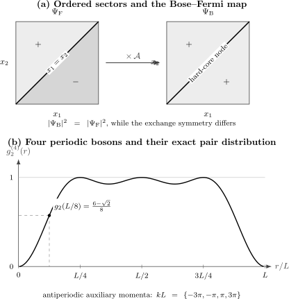
The Bose–Fermi map reverses the fermionic sign between ordered sectors while preserving the coincidence node and probability density. For four periodic bosons, the auxiliary fermions are antiperiodic; their finite-ring kernel gives the plotted pair-correlation hole and the exact value $g_2(L/8)=(6-\sqrt2)/8$.

Static-structure checkpoints

At ring momentum transfer

$$q_\ell = \frac{2\pi\ell}{L},$$

the connected static structure factor is

$$S_\ell = \min\left( \frac{|\ell|}{4}, 1 \right).$$

Thus

$$\left( S_0,S_1,S_2,S_3,S_4 \right) = \left( 0,\frac14,\frac12,\frac34,1 \right).$$

Benchmark contract

A reproducible implementation should report:

1. $N=4$, $m$, $L$, and $E_L=\hbar^2/(2mL^2)$;
2. periodic bosonic boundary conditions;
3. antiperiodic auxiliary fermion boundary conditions;
4. occupied momenta $kL=\{-3\pi,-\pi,\pi,3\pi\}$;
5. total momentum and energy;
6. normalization and orthogonality errors of the orbitals;
7. $g_2(r)$ at $r=0,L/8,L/4$;
8. the small-$r$ quadratic coefficient;
9. $S_\ell$ for at least $\ell=0,\ldots,4$;
10. grid or quadrature refinement if correlations are evaluated numerically.

The density-kernel identity provides an independent route to the pair distribution. A code that obtains the energy but misses the parity twist may still fail the correlation and momentum-grid checks.

Numerical and Analytical Methods

Orbital propagation

For arbitrary one-body $V(x,t)$, solve

$$i\hbar\partial_t\phi_a = \left[ -\frac{\hbar^2}{2m}\partial_x^2 + V(x,t) \right] \phi_a.$$

Maintain orbital orthonormality, construct the fermionic projector, and use the mapping for the desired bosonic observable. Split-operator, spectral, finite-element, and Crank–Nicolson methods are all suitable when their boundary and convergence errors are controlled.

Determinant formulas

Density observables use the one-particle projector directly. The bosonic one-body density matrix requires a string-dressed determinant. Stable implementations monitor matrix conditioning, particle-number sum rules, Hermiticity, and positive semidefiniteness before Fourier transforming to momentum space.

Finite-coupling comparison

Bethe-root solvers, quantum Monte Carlo, and continuum tensor-network methods can approach the hard-core result from finite $\gamma$. A meaningful comparison holds density and geometry fixed and extrapolates both energy and local correlations.

Lattice regularization

A dilute hard-core lattice-boson chain can regularize the continuum problem. One must extrapolate lattice spacing to zero while holding the physical density and mass fixed. Merely increasing the onsite repulsion at fixed lattice filling tests the lattice hard-core model, not automatically the continuum gas.

Model Boundaries

• Tonks–Girardeau versus Lieb–Liniger: the former is the exact impenetrable limit; the latter contains the full finite-coupling crossover.
• Bosons versus auxiliary fermions: spectra and coordinate-diagonal probabilities agree, but exchange symmetry and off-diagonal fields do not.
• Continuum versus lattice hard core: the continuum has quadratic unbounded dispersion; the lattice has a band and commensurability.
• Point hard core versus hard rods: finite rod length changes the equation of state.
• Repulsive Tonks versus super-Tonks: the super-Tonks gas is an excited attractive branch.
• Spinless versus spinor gas: internal states add exchange-sector dynamics.
• One dimension versus higher dimensions: the ordered-sector mapping is special to one dimension.

Common Mistakes

• Replacing $\Psi_{\mathrm B}$ by $\Psi_{\mathrm F}$ instead of multiplying by the mapping sign.
• Using $\Psi_{\mathrm B}=|\Psi_{\mathrm F}|$ for arbitrary complex excited or time-dependent states.
• Claiming that bosonic and fermionic momentum distributions are equal.
• Omitting the parity-dependent fermion boundary condition on a ring.
• Treating a large but finite $\gamma$ as exactly impenetrable.
• Setting the Tan contact to zero because $g_2(0)=0$.
• Writing a continuum nilpotency condition as though point fields were ordinary bounded operators.
• Equating continuum and lattice hard-core bosons at arbitrary density.
• Calling a finite-diameter hard-rod gas the pointlike Tonks–Girardeau model.
• Applying the mapping unchanged in two or three dimensions.

Summary

• The model consists of one-dimensional bosons with exact coincidence nodes.
• Girardeau’s sign map turns free spinless-fermion solutions into symmetric hard-core-boson solutions.
• Periodic bosons map to periodic fermions for odd $N$ and antiperiodic fermions for even $N$.
• Spectra, thermodynamics, density profiles, and density correlations fermionize exactly.
• One-body coherence and momentum distributions retain a nonlocal bosonic string.
• The uniform gas has free-fermion pressure, $v_s=\hbar\pi n/m$, $K=1$, and a quadratic pair-correlation hole.
• The four-boson ring benchmark fixes the parity sector, energy, pair distribution, and static structure factor.

Exercises

1. Verify the mapping symmetry

Show that

$$\Psi_{\mathrm B} = \mathcal A\Psi_{\mathrm F}$$

is symmetric and satisfies the hard-core node when $\Psi_{\mathrm F}$ is antisymmetric.

Solution

Under exchange of two coordinates, both $\mathcal A$ and $\Psi_{\mathrm F}$ change sign. Their product is unchanged:

$$(-\mathcal A)(-\Psi_{\mathrm F}) = \mathcal A\Psi_{\mathrm F}.$$

Thus $\Psi_{\mathrm B}$ is bosonic. At $x_j=x_\ell$, antisymmetry requires

$$\Psi_{\mathrm F}(\ldots,x_j,\ldots,x_j,\ldots) =0.$$

Therefore the mapped state also vanishes. Inside any ordered sector $\mathcal A$ is constant, so derivatives act only on $\Psi_{\mathrm F}$ and the free Schrödinger equation is preserved away from the nodes.

2. Derive the ring boundary twist

Using $\mathcal A_L$, wind one coordinate by $L$ and determine the mapped fermion boundary condition for odd and even $N$.

Solution

Each factor involving $x_j$ transforms as

$$\begin{gathered} \sin\left[ \frac{\pi(x_j+L-x_\ell)}L \right] \\ = -\sin\left[ \frac{\pi(x_j-x_\ell)}L \right]. \end{gathered}$$

There are $N-1$ such factors, so

$$\begin{gathered} \mathcal A_L(\ldots,x_j+L,\ldots) \\ = (-1)^{N-1} \mathcal A_L(\ldots,x_j,\ldots). \end{gathered}$$

Periodic $\Psi_{\mathrm B}=\mathcal A_L\Psi_{\mathrm F}$ then requires

$$\begin{gathered} \Psi_{\mathrm F}(\ldots,x_j+L,\ldots) \\ = (-1)^{N-1} \Psi_{\mathrm F}(\ldots,x_j,\ldots). \end{gathered}$$

For odd $N$, $N-1$ is even and the fermions are periodic. For even $N$, they are antiperiodic.

3. Compare two particles in a box

Derive the Tonks–Girardeau ground-state energy and density for two particles in a hard-wall box, and compare the energy with ideal bosons.

Solution

The mapped fermions occupy $\phi_1$ and $\phi_2$, whose energies are

$$\epsilon_1 = \pi^2E_L, \qquad \epsilon_2 = 4\pi^2E_L.$$

Hence

$$E_{\mathrm{TG}} = 5\pi^2E_L.$$

The density is the diagonal of the occupied-orbital projector:

$$\begin{aligned} n(x) ={}& |\phi_1(x)|^2 + |\phi_2(x)|^2 \\ ={}& \frac2L \Bigg[ \sin^2\left( \frac{\pi x}{L} \right) \\ &\qquad+ \sin^2\left( \frac{2\pi x}{L} \right) \Bigg]. \end{aligned}$$

Two ideal bosons both occupy $\phi_1$, so

$$E_{\mathrm{ideal}} = 2\pi^2E_L.$$

The difference is the kinetic cost of the hard-core nodal structure.

4. Derive the general ring energy

Show for both parities of $N$ that

$$\frac{E_0}{E_L} = \frac{\pi^2}{3} N(N^2-1).$$

Solution

For odd $N=2M+1$, occupy periodic momenta $k_mL=2\pi m$ with $m=-M,\ldots,M$. Then

$$\begin{aligned} \frac{E_0}{E_L} &= 4\pi^2 \sum_{m=-M}^{M}m^2 \\ &= 8\pi^2 \sum_{m=1}^{M}m^2. \end{aligned}$$

Using

$$\sum_{m=1}^{M}m^2 = \frac{M(M+1)(2M+1)}6$$

and $N=2M+1$ gives the result.

For even $N=2M$, occupy antiperiodic momenta

$$kL = \pm\pi,\pm3\pi,\ldots, \pm(2M-1)\pi.$$

Therefore

$$\frac{E_0}{E_L} = 2\pi^2 \sum_{j=1}^{M} (2j-1)^2.$$

Since

$$\sum_{j=1}^{M}(2j-1)^2 = \frac{M(4M^2-1)}3,$$

the same formula follows after substituting $N=2M$.

5. Reproduce the four-particle pair checkpoints

Starting from $K_4(r)$, derive $g_2^{(4)}(r)$ and evaluate it at $r=L/8$ and $L/4$.

Solution

For a Slater determinant,

$$\langle n(x)n(x+r)\rangle = n^2-|K_4(r)|^2$$

away from the self-correlation. Dividing by $n^2=(4/L)^2$ gives

$$g_2^{(4)}(r) = 1- \left[ \frac{\sin(4\pi r/L)} {4\sin(\pi r/L)} \right]^2.$$

At $r=L/8$,

$$\begin{gathered} \sin\left(\frac\pi2\right)=1, \\ \sin^2\left(\frac\pi8\right) = \frac{2-\sqrt2}{4}. \end{gathered}$$

Thus

$$\begin{aligned} g_2^{(4)}\left(\frac L8\right) &= 1- \frac{1}{ 16\sin^2(\pi/8) } \\ &= \frac{6-\sqrt2}{8}. \end{aligned}$$

At $r=L/4$, the numerator is $\sin\pi=0$, so $g_2^{(4)}(L/4)=1$.

6. Classify observables under the map

For each quantity, state whether it equals the free-fermion result: energy, density, pair distribution, one-body density matrix, momentum distribution, and pressure.

Solution

Energy and pressure agree because the spectra agree. Density and pair distribution agree because they are diagonal functions of particle coordinates and $\mathcal A^2=1$.

The one-body density matrix does not agree: removing a boson at one point and inserting it at another crosses a coordinate-dependent parity string. Its Fourier transform, the bosonic momentum distribution, therefore also differs.

The classification is:

Quantity	Equality
energy	yes
density	yes
pair distribution	yes
one-body density matrix	no
momentum distribution	no
pressure	yes

Cross-Links

• Lieb–Liniger Model Preview — finite repulsion, Bethe roots, thermodynamics, and strong-coupling approach.
• Low-Dimensional Quantum Gases — confinement, dimensional crossover, and experimental setting.
• Luttinger Liquid Preview — the $K=1$ infrared fixed point and algebraic exponents.
• Jordan–Wigner Transformation — lattice parity strings and boundary sectors.
• Exact Solutions Preview — exactness taxonomy and free-mode mappings.
• Correlation Functions Overview — connected correlators and normalization conventions.
• Off-Diagonal Long-Range Order — condensate criteria and reduced density matrices.
• Quantum Quenches — protocol specification and nonequilibrium observables.
• Common Many-Body Hamiltonians — compact continuum and lattice convention lookup.

References

1. L. Tonks, “The Complete Equation of State of One, Two and Three-Dimensional Gases of Hard Elastic Spheres”, Physical Review 50, 955–963 (1936) — classical hard-core gas whose name survives in the quantum regime.
2. M. Girardeau, “Relationship between Systems of Impenetrable Bosons and Fermions in One Dimension”, Journal of Mathematical Physics 1, 516–523 (1960) — rigorous Bose–Fermi mapping and observable distinctions.
3. A. Lenard, “Momentum Distribution in the Ground State of the One-Dimensional System of Impenetrable Bosons”, Journal of Mathematical Physics 5, 930–943 (1964) — one-body density matrix and momentum distribution.
4. H. G. Vaidya and C. A. Tracy, “One-Particle Reduced Density Matrix of Impenetrable Bosons in One Dimension at Zero Temperature”, Physical Review Letters 42, 3–6 (1979) — long-distance asymptotics.
5. E. H. Lieb and W. Liniger, “Exact Analysis of an Interacting Bose Gas. I. The General Solution and the Ground State”, Physical Review 130, 1605–1616 (1963) — finite-coupling parent model.
6. M. Olshanii, “Atomic Scattering in the Presence of an External Confinement and a Gas of Impenetrable Bosons”, Physical Review Letters 81, 938–941 (1998) — confinement-induced one-dimensional coupling.
7. V. Dunjko, V. Lorent, and M. Olshanii, “Bosons in Cigar-Shaped Traps: Thomas–Fermi Regime, Tonks–Girardeau Regime, and In Between”, Physical Review Letters 86, 5413–5416 (2001) — trapped crossover and experimental criteria.
8. B. Paredes et al., “Tonks–Girardeau Gas of Ultracold Atoms in an Optical Lattice”, Nature 429, 277–281 (2004) — experimental realization and momentum-profile evidence.
9. T. Kinoshita, T. Wenger, and D. S. Weiss, “Observation of a One-Dimensional Tonks–Girardeau Gas”, Science 305, 1125–1128 (2004) — continuum-tube experiment.
10. A. Minguzzi and D. M. Gangardt, “Exact Coherent States of a Harmonically Confined Tonks–Girardeau Gas”, Physical Review Letters 94, 240404 (2005) — scaling dynamics and dynamical fermionization.
11. R. Pezer and H. Buljan, “Momentum Distribution Dynamics of a Tonks–Girardeau Gas: Bragg Reflections of a Quantum Many-Body Wave Packet”, Physical Review Letters 98, 240403 (2007) — determinant method for the bosonic one-body density matrix.
12. M. A. Cazalilla, R. Citro, T. Giamarchi, E. Orignac, and M. Rigol, “One Dimensional Bosons: From Condensed Matter Systems to Ultracold Gases”, Reviews of Modern Physics 83, 1405–1466 (2011) — broad review of exact models, Luttinger physics, and experiments.