Hubbard Chain

One-Sentence Description

The Hubbard chain is the uniform one-dimensional lattice model in which spin-$1/2$ fermions hop between neighboring sites and interact only through onsite double occupancy; its standard periodic form is integrable by the nested Bethe ansatz.

This dossier fixes the chain conventions, records the Lieb–Wu equations and exact thermodynamic fingerprints, distinguishes charge and spin gaps, maps the repulsive strong-coupling sector to the Heisenberg chain, and hands finite numerics to MB-B004. The Hubbard Model teaching article remains the canonical home for the general lattice derivation, model-building assumptions, and wider Hubbard family.

Baseline Model Record

Unless a variant is stated explicitly, the exact chain discussion uses:

Field	Baseline choice
lattice	one-dimensional chain of even length $L$ and spacing $a$
physical modes	one spin-$\uparrow$ and one spin-$\downarrow$ fermionic mode per site
boundary condition	periodic, $c_{L+1,\sigma}=c_{1,\sigma}$
hopping	uniform, real $t>0$, nearest neighbors only
interaction	uniform onsite $U\in\mathbb R$
Hamiltonian convention	unshifted fixed-number Hamiltonian $H$, with no chemical-potential term
conserved populations	$N_\uparrow$, $N_\downarrow$, and $N=N_\uparrow+N_\downarrow$
filling	$n=N/L$, with half filling at $n=1$
primary exact regime	repulsive $U>0$, zero field, $N=L$, $N_\uparrow=N_\downarrow=L/2$
absent perturbations	disorder, dimerization, longer-range hopping, intersite interaction, flux, and external fields
finite benchmark	a separate open $L=4$ chain with $t=1$, $U=4$, and $(N_\uparrow,N_\downarrow)=(2,2)$

The even-$L$ assumption keeps the periodic ring bipartite and makes the staggered $\eta$-pairing generators single-valued. Many thermodynamic conclusions survive other boundary choices, but the finite-size Bethe equations, momentum sectors, and edge physics do not remain literally unchanged.

Degrees of Freedom and Hilbert Space

The operators obey

$$\begin{aligned} \{c_{j\sigma},c_{\ell\sigma'}^\dagger\} &= \delta_{j\ell}\delta_{\sigma\sigma'}, \\ \{c_{j\sigma},c_{\ell\sigma'}\} &= 0. \end{aligned}$$

Define

$$n_{j\sigma} = c_{j\sigma}^\dagger c_{j\sigma}, \qquad n_j = n_{j\uparrow}+n_{j\downarrow}.$$

Each site has four local occupation states,

$$\lvert0\rangle_j, \qquad \lvert\uparrow\rangle_j, \qquad \lvert\downarrow\rangle_j, \qquad \lvert\uparrow\downarrow\rangle_j.$$

Consequently,

$$\dim\mathcal F = 4^L.$$

For spin-conserving hopping, the fixed-population sector has dimension

$$\dim\mathcal H_{N_\uparrow,N_\downarrow} = \binom{L}{N_\uparrow} \binom{L}{N_\downarrow}.$$

At balanced half filling,

$$\dim\mathcal H_{L/2,L/2} = \binom{L}{L/2}^{\!2}.$$

Using Stirling’s formula,

$$\binom{L}{L/2}^{\!2} \sim \frac{2}{\pi L}\,4^L.$$

Translation, spatial inversion, total spin, and discrete symmetries can reduce a finite calculation further. The exponential factor remains; symmetry resolution reorganizes the Hilbert space but does not remove the many-body growth.

For bit-based exact diagonalization, a declared mode order is mandatory. The benchmark below uses site-major order,

$$(1\uparrow,1\downarrow,2\uparrow,2\downarrow,\ldots,L\uparrow,L\downarrow).$$

Changing this order changes matrix signs and basis coordinates, not physical eigenvalues, provided every operator is transformed consistently.

Hamiltonian

The baseline fixed-number Hamiltonian is

$$\begin{aligned} H ={}& -t \sum_{j=1}^{L} \sum_{\sigma=\uparrow,\downarrow} \left( c_{j\sigma}^\dagger c_{j+1,\sigma} + c_{j+1,\sigma}^\dagger c_{j\sigma} \right) \\ &+ U \sum_{j=1}^{L} n_{j\uparrow}n_{j\downarrow}. \end{aligned}$$

There are $L$ undirected bonds on a periodic ring. The displayed formula traverses each bond once and writes both hopping directions explicitly. For an open chain, the bond sum ends at $L-1$.

The kinetic and interaction pieces are

$$H = T+UD,$$

with

$$\begin{aligned} T &= -t \sum_{j,\sigma} \left( c_{j\sigma}^\dagger c_{j+1,\sigma} + \mathrm{h.c.} \right), \\ D &= \sum_j n_{j\uparrow}n_{j\downarrow}. \end{aligned}$$

The dimensionless coupling is $U/t$. Filling, magnetization, temperature, and boundary conditions are independent control data; specifying only $U/t$ does not identify a unique physical problem.

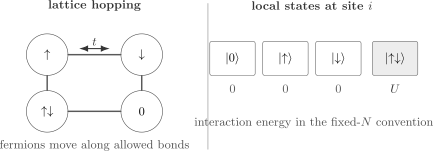
The chain repeats the same local four-state Hilbert space and nearest-neighbor hopping along one dimension. The periodic integrable problem and the open finite benchmark use the same local terms but different boundary bonds.

Momentum-space form

For the periodic chain, use

$$c_{j\sigma} = \frac{1}{\sqrt L} \sum_k e^{ikja} c_{k\sigma}, \qquad k = \frac{2\pi m}{La}.$$

The kinetic term is diagonal:

$$T = \sum_{k,\sigma} \epsilon(k)n_{k\sigma}, \qquad \epsilon(k) = -2t\cos(ka).$$

The onsite interaction transfers momentum between opposite-spin fermions:

$$\begin{aligned} UD ={}& \frac{U}{L} \sum_{k,k',q} c_{k+q,\uparrow}^\dagger c_{k,\uparrow} \\ &\times c_{k'-q,\downarrow}^\dagger c_{k',\downarrow}. \end{aligned}$$

Momentum is conserved modulo a reciprocal lattice vector. The kinetic term is simple in momentum space and the interaction is diagonal in real-space occupation; this incompatible simplicity is the source of the interacting problem.

Centered Convention and Symmetry

On the even bipartite chain, define the centered Hamiltonian

$$\begin{aligned} H_{\mathrm c} ={}& -t \sum_{j,\sigma} \left( c_{j\sigma}^\dagger c_{j+1,\sigma} + \mathrm{h.c.} \right) \\ &+ U \sum_j \left( n_{j\uparrow}-\frac12 \right) \left( n_{j\downarrow}-\frac12 \right). \end{aligned}$$

It differs from the baseline Hamiltonian by number and constant terms:

$$H_{\mathrm c} = H-\frac{U}{2}N+\frac{UL}{4}.$$

Within a fixed-$N$ sector, the two Hamiltonians have identical eigenvectors and differ by a uniform energy shift. Across particle-number sectors, the shift matters and must be restored before defining chemical potentials or addition gaps.

Charge and spin

The total particle number

$$N = \sum_j n_j$$

generates charge $U(1)$. Spin rotations are generated by

$$\begin{aligned} S^+ &= \sum_j c_{j\uparrow}^\dagger c_{j\downarrow}, \\ S^- &= \left(S^+\right)^\dagger, \\ S^z &= \frac12 \sum_j \left( n_{j\uparrow}-n_{j\downarrow} \right). \end{aligned}$$

For spin-independent hopping and no magnetic field,

$$[H,\mathbf S] = 0.$$

The separate conservation of $N_\uparrow$ and $N_\downarrow$ is compatible with this larger spin $SU(2)$ symmetry: $N$ and $S^z$ label convenient sectors, while $S^\pm$ connect sectors with different $S^z$ inside one spin multiplet.

Eta-pairing symmetry

The staggered pair generators are

$$\begin{aligned} \eta^+ &= \sum_{j=1}^{L} (-1)^j c_{j\uparrow}^\dagger c_{j\downarrow}^\dagger, \\ \eta^- &= \left(\eta^+\right)^\dagger, \\ \eta^z &= \frac12 \left( N-L \right). \end{aligned}$$

They form a second $su(2)$ algebra. For the centered Hamiltonian,

$$[H_{\mathrm c},\boldsymbol\eta] = 0.$$

For the unshifted Hamiltonian,

$$[H,\eta^\pm] = \pm U\eta^\pm.$$

Thus it is imprecise to claim that $\eta^\pm$ commute with every commonly written Hubbard Hamiltonian. The exact internal group of the centered even chain is

$$SO(4) \simeq \frac{ SU(2)_{\mathrm{spin}} \times SU(2)_{\eta} }{ \mathbb Z_2 }.$$

The quotient records that the simultaneous central sign acts trivially on physical states.

Space-time symmetries

With real uniform hopping and periodic boundaries, the model also has:

• translation by one lattice site;
• spatial inversion;
• time-reversal symmetry at zero field and zero flux;
• particle–hole symmetry in the centered bipartite convention.

A partial particle–hole transformation on one spin species maps $U$ to $-U$ and exchanges spin and $\eta$-spin structures. This relation connects repulsive and attractive chains, but observables must be transformed along with the Hamiltonian.

Exact Solution Status

The uniform nearest-neighbor periodic Hubbard chain is integrable. Lieb and Wu reduced its spectral problem to coupled algebraic equations by a nested coordinate Bethe ansatz. This is much stronger than saying that a small matrix can be diagonalized, but it is not the same as having elementary closed formulas for every correlation function.

The exactness boundary is:

Question	Status
finite periodic spectrum	encoded by the Lieb–Wu equations, including real and complex roots
thermodynamic ground state	root-density integral equations; several quantities reduce to one-dimensional integrals
finite-temperature thermodynamics	thermodynamic Bethe ansatz or quantum-transfer-matrix equations
elementary excitations	exact dressed energies, momenta, and scattering data
generic local correlators	not obtained by simply reading roots; often requires additional integrability machinery or asymptotics
open uniform chain	integrable boundary formulations exist, but equations differ from the periodic baseline
dimerization, disorder, generic $t'$, or generic intersite $V$	standard Hubbard integrability is generally lost
ladders and dimensions above one	no generic Lieb–Wu solution

Integrability is a property of a precisely specified Hamiltonian, not of the word “Hubbard.”

Lieb–Wu Equations

Take $N$ particles, of which $M=N_\downarrow$ have down spin, and define

$$u = \frac{U}{4t}.$$

An eigenstate is characterized by $N$ charge momenta $k_j$ and $M$ spin rapidities $\lambda_\alpha$. In one standard convention, they satisfy

$$e^{ik_jL} = \prod_{\alpha=1}^{M} \frac{ \lambda_\alpha-\sin k_j-iu }{ \lambda_\alpha-\sin k_j+iu }, \qquad j=1,\ldots,N,$$

and

$$\begin{aligned} \prod_{j=1}^{N} \frac{ \lambda_\alpha-\sin k_j-iu }{ \lambda_\alpha-\sin k_j+iu } ={}& \prod_{\substack{\beta=1\\\beta\ne\alpha}}^{M} \frac{ \lambda_\alpha-\lambda_\beta-2iu }{ \lambda_\alpha-\lambda_\beta+2iu }, \\ &\alpha=1,\ldots,M. \end{aligned}$$

Here the lattice spacing is absorbed into $k_j$. The energy of the unshifted Hamiltonian and the total crystal momentum are

$$E = -2t \sum_{j=1}^{N} \cos k_j, \qquad P = \frac{1}{a} \left( \sum_{j=1}^{N}k_j \right) \bmod\frac{2\pi}{a}.$$

For the centered Hamiltonian,

$$E_{\mathrm c} = E-\frac{UN}{2}+\frac{UL}{4}.$$

The interaction is absent from the explicit unshifted energy formula but remains fully present in the allowed roots. Replacing interacting roots by free momenta would erase the solution rather than simplify it.

Why the ansatz is nested

The coordinate wavefunction is a superposition of plane waves in each ordering region of particle coordinates. Two-particle scattering changes spin amplitudes, so the spatial momenta do not close on themselves. The first layer quantizes charge motion; an auxiliary spin-chain problem quantizes the spin rapidities. This nested structure is the one-dimensional expression of separate charge and spin organization.

Solutions need not remain real. Complex root patterns encode bound structures, and logarithmic forms require branch choices plus integer or half-integer quantum numbers. Numerical root solving therefore needs:

1. a declared equation convention;
2. a state-counting prescription;
3. control of complex roots and finite-size deviations;
4. comparison with symmetry multiplets or exact diagonalization at small $L$.

Solving one real branch is not a completeness test.

Exact Half-Filled Ground-State Energy

For $U\ge0$, zero field, and half filling, the thermodynamic ground-state energy per site of the unshifted Hamiltonian is

$$e_0(U) = -4t \int_0^\infty \frac{ J_0(\omega)J_1(\omega) }{ \omega \left[ 1+\exp\left( \dfrac{U\omega}{2t} \right) \right] } \,d\omega,$$

where $J_\nu$ is the Bessel function of the first kind. The formula passes two essential limits.

At $U=0$,

$$e_0(0) = -\frac{4t}{\pi},$$

the half-filled tight-binding Fermi-sea energy.

For $U/t\gg1$,

$$e_0(U) = -\frac{4t^2\ln2}{U} + O\!\left( \frac{t^4}{U^3} \right).$$

The leading term equals the ground-state energy density of the effective Heisenberg Hamiltonian in the convention derived below.

Double occupancy

The Feynman–Hellmann theorem gives the thermodynamic double occupancy per site:

$$d(U) \equiv \lim_{L\to\infty} \frac{\langle D\rangle_0}{L} = \frac{\partial e_0}{\partial U}.$$

Differentiating the exact integral,

$$\begin{aligned} d(U) = 2 \int_0^\infty J_0(\omega)J_1(\omega) \frac{ \exp\left( \dfrac{U\omega}{2t} \right) }{ \left[ 1+\exp\left( \dfrac{U\omega}{2t} \right) \right]^2 } \,d\omega. \end{aligned}$$

The limiting values are

$$d(0) = \frac14, \qquad d(U) \sim \frac{4t^2\ln2}{U^2} \quad (U/t\to\infty).$$

Double occupancy is suppressed continuously for repulsive $U$; it does not jump to zero at finite coupling.

Mott Charge Gap

Let $E_0(L,N)$ be the lowest energy at particle number $N$, minimized over spin sectors. The thermodynamic charge gap at half filling is

$$\begin{aligned} \Delta_{\mathrm c} ={}& \lim_{L\to\infty} \Big[ E_0(L,L+1) + E_0(L,L-1) \\ &\hspace{5em} -2E_0(L,L) \Big]. \end{aligned}$$

Equivalently,

$$\Delta_{\mathrm c} = \mu_+-\mu_-,$$

where $\mu_+$ and $\mu_-$ are the particle-addition and particle-removal thresholds. For $U>0$, the exact result is

$$\Delta_{\mathrm c}(U) = \frac{16t^2}{U} \int_1^\infty \frac{ \sqrt{y^2-1} }{ \sinh\left( \dfrac{2\pi t y}{U} \right) } \,dy.$$

The integrand is positive, so

$$\Delta_{\mathrm c}(U)>0 \qquad \text{for every }U>0.$$

There is no metal-to-insulator transition at a finite positive coupling. The critical point is $U=0$: the half-filled chain is metallic there and Mott insulating for every repulsive $U$.

The weak- and strong-coupling asymptotics are

$$\Delta_{\mathrm c}(U) \sim \frac{8}{\pi} \sqrt{Ut}\, \exp\left( -\frac{2\pi t}{U} \right) \qquad (U/t\to0^+),$$

and

$$\Delta_{\mathrm c}(U) = U-4t + \frac{8t^2\ln2}{U} + O\!\left( \frac{t^4}{U^3} \right) \qquad (U/t\to\infty).$$

The exponentially small weak-coupling gap is easy to miss in finite systems. A cluster level spacing of order $v/L$ can exceed the bulk Mott scale unless $L$ is extremely large.

Spin gap

For an even half-filled chain, define

$$\Delta_{\mathrm s}(L) = E_0(L,N=L,S=1) - E_0(L,N=L,S=0).$$

For repulsive $U>0$,

$$\lim_{L\to\infty} \Delta_{\mathrm s}(L) = 0.$$

The half-filled repulsive chain is therefore charge gapped and spin gapless. “The Hubbard chain is gapped” is incomplete unless the excitation channel is named.

Spin–Charge Separation

The Bethe solution organizes excitations into charge and spin sectors. At repulsive half filling:

• holons and antiholons carry charge but no spin and are gapped;
• spinons carry spin $1/2$ but no charge and are gapless;
• physical finite-volume states obey selection rules and are assembled from allowed combinations of these elementary excitations.

This does not mean that an electron operator factors into two independent particles at every microscopic scale. It means that the low-energy spectral organization and propagation separate into collective charge and spin channels with different quantum numbers and, away from the charge-gapped point, generally different velocities.

Away from half filling, both channels are gapless for the repulsive zero-field chain. The low-temperature free-energy density has the universal two-mode form

$$f(T) = e_0 - \frac{\pi(k_{\mathrm B}T)^2}{6} \left( \frac{1}{v_{\mathrm c}} + \frac{1}{v_{\mathrm s}} \right) + o(T^2),$$

with charge and spin velocities $v_{\mathrm c}$ and $v_{\mathrm s}$. At half filling with $U>0$, the charge contribution is exponentially suppressed at temperatures well below $\Delta_{\mathrm c}$, while the gapless spin channel remains.

Regime Map

At zero field and in the thermodynamic limit, the standard uniform chain has the following low-energy structure:

Coupling and filling	Charge sector	Spin sector	Low-energy description
$U=0$, $0<n<2$	gapless	gapless	two-flavor free Fermi gas
$U>0$, $n=1$	gapped	gapless	one-dimensional Mott insulator; critical spin sector
$U>0$, $n\ne1$	gapless	gapless	spinful Luttinger liquid
$U<0$, generic filling	gapless	gapped	Luther–Emery liquid with paired correlations
$U<0$, $n=1$	gapless	gapped	charge-density-wave and onsite-pair correlations related by $\eta$-spin symmetry
$n=0$ or $n=2$	trivial vacuum or filled state	no low-energy spin mode	band endpoint

The words “metal,” “insulator,” and “paired” refer here to thermodynamic response and correlation structure. The one-dimensional short-range chain does not acquire conventional finite-temperature long-range order merely because a correlation channel is dominant.

Correlation hierarchy

For repulsive $U>0$ away from half filling, spin-density-wave correlations are enhanced relative to free fermions, but all standard order parameters have vanishing expectation value in the symmetry-preserving thermodynamic ground state. Correlations decay algebraically.

For attractive $U<0$, a spin gap suppresses single-particle and spin excitations at low energy. Singlet-pair and charge-density correlations decay algebraically. At half filling, the $\eta$-spin symmetry makes the corresponding charge-density-wave and onsite-pair exponents degenerate.

These statements concern asymptotic correlations. They do not identify a finite system’s largest structure-factor peak as spontaneous order.

Important Limits

Noninteracting limit

At $U=0$, each spin species occupies the tight-binding band

$$\epsilon(k) = -2t\cos(ka).$$

For a spin-balanced state with $0<n<2$,

$$k_{\mathrm F} = \frac{\pi n}{2a}.$$

At half filling,

$$k_{\mathrm F} = \frac{\pi}{2a}, \qquad v_{\mathrm F} = \frac{1}{\hbar} \left. \frac{d\epsilon}{dk} \right|_{k_{\mathrm F}} = \frac{2ta}{\hbar}.$$

The band is half occupied, not full.

Atomic limit

At $t=0$, sites decouple. At half filling and $U>0$, configurations with exactly one fermion per site have zero interaction energy in the unshifted convention. Their spin orientations are degenerate:

$$\dim\mathcal H_{\mathrm{atomic,low}} = 2^L.$$

Any doublon requires a compensating empty site and costs $U$. Infinitesimal nonzero hopping does not simply restore free motion; at second order it lifts the spin degeneracy through antiferromagnetic exchange.

Repulsive strong coupling

At $N=L$ and $U/t\gg1$, project onto the subspace with one fermion per site. A virtual hop creates a doublon–holon pair of energy $U$, and a second hop removes it. To order $t^2/U$,

$$H_{\mathrm{eff}} = J \sum_{j=1}^{L} \left( \mathbf S_j\cdot\mathbf S_{j+1} - \frac14 \right), \qquad J = \frac{4t^2}{U}.$$

The $-1/4$ term matters when comparing absolute Hubbard energies. The antiferromagnetic Heisenberg ground-state energy per bond is

$$J \left( \frac14-\ln2 \right).$$

Including the subtraction in $H_{\mathrm{eff}}$ gives

$$\frac{E_0}{L} \sim -J\ln2 = -\frac{4t^2\ln2}{U},$$

exactly matching the large-$U$ expansion of the Lieb–Wu integral.

This effective model describes low-energy spin dynamics below the charge scale. It does not reproduce doublon production, charge transport across the Mott gap, or high-energy Hubbard bands.

Infinite repulsion

For densities below half filling, $U/t\to\infty$ forbids double occupancy but does not freeze charge because holes remain. Charge coordinates behave like constrained spinless fermions, while the spin sector becomes highly degenerate at strictly infinite $U$ because $J\to0$. Taking $U\to\infty$ before or after probing the spin scale can therefore give different-looking limits.

Attractive coupling

For $U<0$, onsite singlet pairs are energetically favored. In the strong-attraction limit, breaking a pair costs order $\lvert U\rvert$, while pair motion appears at order $t^2/\lvert U\rvert$. The partial particle–hole map relates this spin-gapped problem to charge localization in the repulsive model.

Typical Observables

No single observable diagnoses every regime. A reliable analysis combines conserved-sector energies, local fluctuations, correlation functions, and finite-size scaling.

Density, magnetization, and double occupancy

The filling and magnetization density are

$$n = \frac{\langle N\rangle}{L}, \qquad m = \frac{ \langle N_\uparrow-N_\downarrow\rangle }{2L}.$$

The double occupancy per site is

$$d = \frac{1}{L} \sum_j \langle n_{j\uparrow}n_{j\downarrow} \rangle.$$

The local-moment diagnostic obeys

$$\begin{aligned} \left\langle \left( n_{j\uparrow}-n_{j\downarrow} \right)^2 \right\rangle ={}& \langle n_j\rangle \\ &- 2 \langle n_{j\uparrow}n_{j\downarrow} \rangle. \end{aligned}$$

At half filling in a translation-invariant state, this becomes $1-2d$. A large local moment indicates suppressed double occupancy; it does not by itself prove magnetic long-range order.

Charge and spin correlations

Useful connected equal-time correlators are

$$C_{\mathrm c}(r) = \left\langle \left( n_{j+r}-n \right) \left( n_j-n \right) \right\rangle,$$

and

$$C_{\mathrm s}(r) = \langle S_{j+r}^zS_j^z \rangle - \langle S_{j+r}^z\rangle \langle S_j^z\rangle.$$

One Fourier convention is

$$S_\alpha(q) = \sum_r e^{-iqra} C_\alpha(r), \qquad \alpha\in\{\mathrm c,\mathrm s\}.$$

The normalization must be stated before comparing values across codes or papers.

Pair correlations

For onsite singlet pairs,

$$\Delta_j = c_{j\downarrow}c_{j\uparrow},$$

and

$$P(r) = \langle \Delta_{j+r}^\dagger\Delta_j \rangle.$$

Repulsive and attractive chains exchange the roles of selected spin and pairing or charge correlations under the partial particle–hole transformation.

Momentum distribution and spectral function

The momentum distribution is

$$n_\sigma(k) = \langle c_{k\sigma}^\dagger c_{k\sigma} \rangle.$$

For an interacting one-dimensional metal, $n(k)$ has no Landau-quasiparticle jump. Its nonanalyticity is instead governed by Luttinger-liquid exponents.

The single-particle spectral function resolves electron addition and removal. Spin–charge separation appears through continua and threshold structures rather than a single free-electron dispersion. Computing these functions is substantially harder than solving the ground-state root density.

Response coefficients

The zero-temperature compressibility and spin susceptibility probe the charge and spin channels:

$$\kappa = \frac{1}{n^2} \frac{\partial n}{\partial\mu}, \qquad \chi_{\mathrm s} = \frac{\partial m}{\partial h}.$$

At repulsive half filling, the charge gap implies zero compressibility in the thermodynamic zero-temperature limit, while the gapless spin sector has a nonzero spin response subject to logarithmic corrections.

Boundary twists can define charge and spin stiffnesses through ground-state curvature. The twist convention, order of limits, and distinction between Drude weight and static susceptibility must be explicit.

Minimal Worked Example: Half Filling at Zero Interaction

Set $U=0$ and take the thermodynamic limit. Both spin species fill

$$-k_{\mathrm F} \le k \le k_{\mathrm F}, \qquad k_{\mathrm F} = \frac{\pi}{2a}.$$

The energy per site is

$$\begin{aligned} e_0(0) &= 2 \frac{a}{2\pi} \int_{-k_{\mathrm F}}^{k_{\mathrm F}} \left[ -2t\cos(ka) \right] \,dk \\ &= -\frac{4t}{\pi}. \end{aligned}$$

The two spin occupations factorize. At half filling,

$$\langle n_{j\uparrow}\rangle = \langle n_{j\downarrow}\rangle = \frac12,$$

so

$$d(0) = \langle n_{j\uparrow}n_{j\downarrow}\rangle = \frac14.$$

These values anchor the exact interacting formulas. Any implementation of the half-filled integral should approach $-4t/\pi$ and $1/4$ continuously as $U\to0^+$.

On a finite periodic ring, the allowed momenta may place a level exactly at the Fermi points. Ground-state degeneracy then depends on $L\bmod4$ and on the boundary twist. That shell effect is a finite-size convention, not a bulk gap.

Numerical Benchmark: MB-B004

The stable finite benchmark is not the periodic Bethe-ansatz baseline. It is an open four-site chain with bonds

$$(1,2), \qquad (2,3), \qquad (3,4),$$

site-major mode ordering, and

$$t=1, \qquad U=4, \qquad N_\uparrow=N_\downarrow=2.$$

The sector dimension is

$$\binom42 \binom42 = 36.$$

Dense diagonalization should reproduce

$$\begin{aligned} E_0 &= -1.953145308684556, \\ E_1 &= -1.412898695919094, \\ E_1-E_0 &= 0.540246612765462. \end{aligned}$$

For

$$D = \sum_{j=1}^{4} n_{j\uparrow}n_{j\downarrow},$$

the trusted ground-state value is

$$\langle D\rangle_0 = 0.339585650339361.$$

The interaction and kinetic energies are

$$\begin{aligned} E_{\mathrm{int}} &= U\langle D\rangle_0 = 1.358342601357445, \\ E_{\mathrm{kin}} &= E_0-E_{\mathrm{int}} = -3.311487910042001. \end{aligned}$$

Whole-block traces test matrix assembly independently of the lowest eigenpair:

$$\operatorname{Tr}H = 144,$$

and

$$\frac{1}{36} \operatorname{Tr}H^2 = 25.3333333333333.$$

A serious benchmark run should verify:

1. the $36$-state basis count;
2. Hermiticity and closure of the fixed-$(N_\uparrow,N_\downarrow)$ sector;
3. $E_0$, $E_1$, the trace, and the quadratic moment;
4. double occupancy both directly and through the energy decomposition;
5. invariance under a consistently changed mode ordering;
6. agreement between two independently assembled Hamiltonian representations.

The number $E_1-E_0$ is the first spacing inside one finite open-chain symmetry block. It is not the thermodynamic charge gap, spin gap, optical gap, or unrestricted many-body gap.

Finite-Size Interpretation

Finite chains mix several scales:

$$\Delta_{\mathrm{finite}} \sim \frac{\hbar v}{L}, \qquad \Delta_{\mathrm c}, \qquad J \sim \frac{4t^2}{U}.$$

At weak positive $U$, $\Delta_{\mathrm c}$ is exponentially small and can be hidden below the finite-size spacing. At strong coupling, charge excitations remain expensive while the spin spacing scales with $J/L$. A single finite-size gap curve therefore cannot identify the bulk sector without quantum numbers and scaling.

Useful extrapolations keep separate:

• even and odd sizes;
• $L\bmod4$ shell families for periodic free-fermion ancestry;
• open and periodic boundaries;
• fixed-particle and grand-canonical gaps;
• spin-singlet, spin-triplet, particle-addition, and particle-removal sectors.

The Finite-Size Scaling in Numerics page owns general extrapolation methods.

Variants and Integrability Hazards

Variant	Hamiltonian change	Main consequence
boundary twist	$c_{L+1,\sigma}=e^{i\phi_\sigma}c_{1,\sigma}$	probes charge or spin stiffness and changes finite-size quantization
open ends	remove the $(L,1)$ bond	translation is lost; boundary Bethe ansatz or open-chain numerics are required
next-neighbor hopping	add $t'$	breaks bipartiteness and generic Lieb–Wu integrability
dimerized hopping	alternate $t_1,t_2$	doubles the unit cell and can open a one-body gap
intersite interaction	add $V\sum_j n_jn_{j+1}$	extended Hubbard chain with additional competing phases
ionic potential	add $\Delta\sum_j(-1)^j n_j$	ionic Hubbard model; band and interaction-driven localization compete
spin imbalance or field	add $-hS^z$	changes root distributions and velocities
disorder	random hopping or onsite energy	translation and standard integrability are lost
coupled chains	add transverse hopping	ladder physics; no generic one-chain Bethe solution
higher dimension	change lattice graph	thermodynamic physics is qualitatively different and generally numerical

Small perturbations can preserve a low-energy universality class while destroying exact integrability. “Not Bethe solvable” does not mean “physically unrelated,” and “close to integrable” does not make the unperturbed exact formulas numerically exact for the perturbed Hamiltonian.

Physical Phenomena

The baseline chain is a controlled arena for:

• interaction-driven charge localization without a finite positive critical $U$;
• a gapless spin channel coexisting with a charge gap;
• spin–charge separation and distinct propagation velocities;
• nonperturbative weak-coupling gap generation by commensurate umklapp scattering;
• antiferromagnetic superexchange at large repulsion;
• Luttinger- and Luther–Emery-liquid correlation structure;
• exact thermodynamic and excitation benchmarks for approximate methods.

It is not, by itself, a quantitatively complete model of a particular material. Real systems can require multiple orbitals, longer-range Coulomb terms, electron–phonon coupling, interchain hopping, disorder, and three-dimensional environments.

Common Mistakes

• Calling $n=1$ full filling. Two spin modes live on each site, so full filling is $n=2$.
• Quoting a phase from $U/t$ alone without specifying filling, magnetization, temperature, and boundary conditions.
• Mixing the unshifted and centered Hamiltonians when comparing energies across particle-number sectors.
• Claiming $[H,\eta^\pm]=0$ for the unshifted Hamiltonian; the commuting $SU(2)_\eta$ generators belong to the centered convention.
• Treating the explicit Bethe energy $-2t\sum_j\cos k_j$ as a free-particle result while ignoring the interaction-dependent roots.
• Assuming every Bethe root is real or that one numerical root branch gives the complete spectrum.
• Saying the repulsive half-filled chain has “a gap” without distinguishing its positive charge gap from its vanishing spin gap.
• Interpreting an open four-site block spacing as the thermodynamic Mott gap.
• Applying $J=4t^2/U$ to charge dynamics or to intermediate coupling without an error estimate.
• Inferring magnetic long-range order from a growing antiferromagnetic structure factor in a short chain.
• Carrying periodic-ring bond counting into the $L=2$ dimer, where careless directed sums can double the sole physical bond.
• Assuming a next-neighbor, disordered, dimerized, ladder, or higher-dimensional Hubbard model retains the standard Lieb–Wu solution.

Exercises

1. Convention shift and Bethe energy

Show that the centered and unshifted Hamiltonians satisfy

$$H_{\mathrm c} = H-\frac{U}{2}N+\frac{UL}{4}.$$

Starting from

$$E_{\mathrm c} = -2t\sum_j\cos k_j + \frac{U}{4}(L-2N),$$

recover the energy of the unshifted Hamiltonian.

Solution

Expand one centered onsite term:

$$\left( n_{j\uparrow}-\frac12 \right) \left( n_{j\downarrow}-\frac12 \right) = n_{j\uparrow}n_{j\downarrow} - \frac12 n_j + \frac14.$$

Summing over sites gives

$$H_{\mathrm c} = H-\frac{U}{2}N+\frac{UL}{4}.$$

Therefore

$$E = E_{\mathrm c} + \frac{UN}{2} - \frac{UL}{4}.$$

Substituting the centered Bethe energy,

$$\begin{aligned} E ={}& -2t\sum_j\cos k_j + \frac{U}{4}(L-2N) \\ &+ \frac{UN}{2} - \frac{UL}{4} \\ ={}& -2t\sum_j\cos k_j. \end{aligned}$$

The cancellation removes only explicit constants. The roots $k_j$ still depend on $U$ through the Lieb–Wu equations.

2. Free half-filled fingerprints

Derive

$$e_0(0) = -\frac{4t}{\pi}$$

and

$$d(0) = \frac14$$

for the spin-balanced thermodynamic ground state.

Solution

At half filling each spin species occupies $-k_{\mathrm F}\le k\le k_{\mathrm F}$ with $k_{\mathrm F}=\pi/(2a)$. Thus

$$\begin{aligned} e_0(0) &= 2 \frac{a}{2\pi} \int_{-\pi/(2a)}^{\pi/(2a)} -2t\cos(ka)\,dk \\ &= -\frac{4t}{\pi}. \end{aligned}$$

At $U=0$ the up- and down-spin Slater determinants factorize. Translation invariance gives

$$\langle n_{j\uparrow}\rangle = \langle n_{j\downarrow}\rangle = \frac12.$$

Hence

$$d(0) = \langle n_{j\uparrow}\rangle \langle n_{j\downarrow}\rangle = \frac14.$$

3. Weak-coupling charge gap

Use the exact gap integral to recover the leading exponential scale as $U/t\to0^+$. In the dominant region $y\approx1$, use

$$\sqrt{y^2-1} \approx \sqrt{2(y-1)}$$

and

$$\frac{1}{\sinh x} \approx 2e^{-x}.$$

Solution

Let

$$A = \frac{2\pi t}{U} \gg1, \qquad y = 1+s.$$

Then

$$\begin{aligned} \int_1^\infty \frac{\sqrt{y^2-1}}{\sinh(Ay)} \,dy &\sim 2\sqrt2\,e^{-A} \int_0^\infty s^{1/2}e^{-As}\,ds \\ &= 2\sqrt2\,e^{-A} \frac{\Gamma(3/2)}{A^{3/2}} \\ &= \frac{\sqrt{2\pi}}{A^{3/2}} e^{-A}. \end{aligned}$$

Multiplying by $16t^2/U$ and substituting $A=2\pi t/U$ gives

$$\Delta_{\mathrm c} \sim \frac{8}{\pi} \sqrt{Ut}\, \exp\left( -\frac{2\pi t}{U} \right).$$

The nonanalytic exponential explains why no finite order of ordinary perturbation theory in $U$ can generate the Mott gap.

4. Strong-coupling energy match

The spin-$1/2$ antiferromagnetic Heisenberg chain

$$H_{\mathrm H} = J \sum_j \mathbf S_j\cdot\mathbf S_{j+1}$$

has ground-state energy per bond

$$J \left( \frac14-\ln2 \right).$$

Show that the Hubbard effective Hamiltonian reproduces the leading large-$U$ term of $e_0(U)$.

Solution

The projected Hubbard Hamiltonian is

$$H_{\mathrm{eff}} = J \sum_j \left( \mathbf S_j\cdot\mathbf S_{j+1} - \frac14 \right), \qquad J = \frac{4t^2}{U}.$$

For a periodic chain there is one bond per site. Its ground-state energy per site is therefore

$$\begin{aligned} e_{\mathrm{eff}} &= J \left( \frac14-\ln2 \right) - \frac{J}{4} \\ &= -J\ln2 \\ &= -\frac{4t^2\ln2}{U}. \end{aligned}$$

This equals the leading strong-coupling term of the exact Lieb–Wu ground-state energy.

5. Eta symmetry and energy ladders

Assume

$$[H_{\mathrm c},\eta^+] = 0$$

and use

$$H = H_{\mathrm c} + \frac{U}{2}N - \frac{UL}{4}$$

together with $[N,\eta^+]=2\eta^+$ to derive $[H,\eta^+]$. Interpret the result.

Solution

Constants commute with every operator, so

$$\begin{aligned} [H,\eta^+] &= [H_{\mathrm c},\eta^+] + \frac{U}{2} [N,\eta^+] \\ &= 0 + \frac{U}{2} \left( 2\eta^+ \right) \\ &= U\eta^+. \end{aligned}$$

Thus $\eta^+$ maps an eigenstate of the unshifted Hamiltonian to a state two particles higher and energy $U$ higher, when the result is nonzero. In the centered convention the number-dependent offset has been removed, so the same multiplet is degenerate and the $\eta$ generators commute with $H_{\mathrm c}$.

6. Audit the four-site benchmark

At the MB-B004 point, use the quoted double occupancy to compute the interaction and kinetic energies. Then explain why agreement with these two numbers does not by itself validate the whole Hamiltonian.

Solution

With $U=4$,

$$\begin{aligned} E_{\mathrm{int}} &= 4 \left( 0.339585650339361 \right) \\ &= 1.358342601357444, \end{aligned}$$

which differs from the tabulated last digit only by decimal rounding. Therefore

$$\begin{aligned} E_{\mathrm{kin}} &= E_0-E_{\mathrm{int}} \\ &\approx -1.953145308684556 - 1.358342601357444 \\ &= -3.311487910042000. \end{aligned}$$

These checks probe the ground-state eigenpair and the decomposition $H=T+UD$. A matrix could still have incorrect excited states, miss basis states, or accidentally violate the fixed sector while reproducing one optimized energy. The dimension, Hermiticity, closure, $E_1$, $\operatorname{Tr}H$, $\operatorname{Tr}H^2$, and an independently assembled representation test broader parts of the calculation.

Cross-Links

• Model Encyclopedia for the shared dossier contract and solution-status vocabulary.
• Hubbard Model for the canonical model derivation, lattice scope, observables, and material-modeling boundary.
• Hubbard Dimer for the complete two-site spectrum and analytic finite-cluster seed.
• Tight-Binding Chain for the $U=0$ dispersion, boundary phases, and finite-size shell structure.
• Heisenberg Chain for the spin model reached at repulsive half filling and large $U/t$.
• Exact Solutions Preview for Bethe-ansatz concepts and the limits of exact solvability.
• Luttinger-Liquid Preview for the universal gapless theory away from commensurate charge localization.
• Fractionalization for the general local-operator and deconfinement criteria, material probes, and comparison with higher-dimensional topological sectors.
• Effective Hamiltonians in Many-Body Systems for the controlled Hubbard-to-Heisenberg projection.
• Equal-Time Correlations and Structure Factors for observable definitions and normalization.
• Boundary Conditions on Lattices for open, periodic, and twisted finite systems.
• MB-B004 for authoritative inputs, outputs, tolerances, and failure diagnoses.
• Reproducible Notebooks for artifact requirements and release gates.
• Hubbard Model reference card and Hamiltonian card for compact lookup.

References

1. J. Hubbard, “Electron Correlations in Narrow Energy Bands,” Proceedings of the Royal Society A 276, 238–257 (1963), doi:10.1098/rspa.1963.0204.
2. E. H. Lieb and F. Y. Wu, “Absence of Mott Transition in an Exact Solution of the Short-Range, One-Band Model in One Dimension,” Physical Review Letters 20, 1445–1448 (1968), doi:10.1103/PhysRevLett.20.1445.
3. M. Takahashi, “One-Dimensional Hubbard Model at Finite Temperature,” Progress of Theoretical Physics 47, 69–82 (1972), doi:10.1143/PTP.47.69.
4. C. N. Yang, ”$\eta$ Pairing and Off-Diagonal Long-Range Order in a Hubbard Model,” Physical Review Letters 63, 2144–2147 (1989), doi:10.1103/PhysRevLett.63.2144.
5. A. A. Ovchinnikov, “Excitation Spectrum in One-Dimensional Hubbard Model,” Soviet Physics JETP 30, 1160–1169 (1970).
6. F. H. L. Essler, V. E. Korepin, and K. Schoutens, “Complete Solution of the One-Dimensional Hubbard Model,” Physical Review Letters 67, 3848–3851 (1991), doi:10.1103/PhysRevLett.67.3848.
7. F. H. L. Essler, H. Frahm, F. Göhmann, A. Klümper, and V. E. Korepin, The One-Dimensional Hubbard Model, Cambridge University Press (2005), doi:10.1017/CBO9780511534843.
8. T. Deguchi, F. H. L. Essler, F. Göhmann, A. Klümper, V. E. Korepin, and K. Kusakabe, “Thermodynamics and Excitations of the One-Dimensional Hubbard Model,” Physics Reports 331, 197–281 (2000), doi:10.1016/S0370-1573(00)00010-7.
9. E. H. Lieb and F. Y. Wu, “The One-Dimensional Hubbard Model: A Reminiscence,” Physica A 321, 1–27 (2003), doi:10.1016/S0378-4371(02)01785-5.
10. T. Giamarchi, Quantum Physics in One Dimension, Oxford University Press (2004).