Lieb–Liniger Model Preview

One-Sentence Description

The repulsive Lieb–Liniger model is a uniform one-dimensional gas of identical bosons with zero-range pair interactions whose finite-volume spectrum and equilibrium thermodynamics are determined by Bethe ansatz.

Canonical Scope

This dossier is the canonical home for:

• the first- and second-quantized Hamiltonians with a complete coupling dictionary;
• periodic-ring boundary conditions, cusp conditions, symmetries, and control parameters;
• finite-volume Bethe equations and their quantum-number conventions;
• the thermodynamic ground-state and Yang–Yang equations at preview depth;
• the distinction between spectral integrability and correlation-function difficulty;
• an observable–method dictionary;
• an exact two-boson ring benchmark with roots, energy, and contact derivative.

Low-Dimensional Quantum Gases owns dimensional reduction, infrared state counting, and the broader experimental setting. Nonrelativistic Field Theory from Many-Body QM owns the general field-theory bridge. Luttinger Liquid Preview owns the universal long-distance Hamiltonian, the parameter $K$, and correlation exponents.

Tonks–Girardeau Gas Preview owns the hard-core Bose–Fermi mapping, ring parity twist, and observable-by-observable limitations. This page reaches that regime only as the strong-repulsion limit of the finite-coupling model.

The baseline below is $N$ identical spinless bosons on a periodic ring of circumference $L$, repulsive contact coupling $g_{\mathrm{1D}}\gt0$, no external potential, and fixed particle number. The attractive gas, trapped gas, multicomponent gases, and finite-range corrections are separate variants.

Model Definition

First-quantized form

For symmetric wavefunctions

$$\Psi(x_1,\ldots,x_N) = \Psi(x_{P1},\ldots,x_{PN})$$

for every permutation $P$, the Hamiltonian is

$$\begin{aligned} H_{\mathrm{LL}} ={}& -\frac{\hbar^2}{2m} \sum_{j=1}^{N} \frac{\partial^2}{\partial x_j^2} \\ &+ g_{\mathrm{1D}} \sum_{1\le j\lt\ell\le N} \delta(x_j-x_\ell). \end{aligned}$$

Periodic boundary conditions mean

$$\Psi(\ldots,x_j+L,\ldots) = \Psi(\ldots,x_j,\ldots).$$

The particles live in a continuum. There is no lattice spacing, onsite occupation cutoff, or Brillouin zone.

Second-quantized form

Let

$$[\psi(x),\psi^\dagger(y)] = \delta(x-y),$$

with all equal-time field commutators otherwise zero. Then

$$\begin{aligned} H_{\mathrm{LL}} ={}& \int_0^L dx\, \Bigg[ \frac{\hbar^2}{2m} (\partial_x\psi^\dagger) (\partial_x\psi) \\ &\qquad+ \frac{g_{\mathrm{1D}}}{2} \psi^\dagger\psi^\dagger\psi\psi \Bigg]. \end{aligned}$$

The factor $1/2$ prevents double counting of unordered particle pairs. Omitting it while keeping the same symbol $g_{\mathrm{1D}}$ changes the model.

The conserved number operator is

$$N = \int_0^L dx\, \psi^\dagger(x)\psi(x).$$

A grand-canonical calculation uses

$$K = H_{\mathrm{LL}}-\mu N,$$

but the finite-ring Bethe benchmark below works at fixed $N$.

Coupling Dictionary

Define the inverse-length coupling

$$c = \frac{m g_{\mathrm{1D}}}{\hbar^2}.$$

Then

$$g_{\mathrm{1D}} = \frac{\hbar^2c}{m}.$$

Factoring out $\hbar^2/(2m)$ gives the common Bethe-ansatz convention

$$\begin{aligned} H_{\mathrm{LL}} ={}& \frac{\hbar^2}{2m} \Bigg[ -\sum_{j=1}^{N}\partial_{x_j}^2 \\ &\qquad+ 2c \sum_{j\lt\ell} \delta(x_j-x_\ell) \Bigg]. \end{aligned}$$

Thus a paper that writes the dimensionless interaction as $2c\,\delta(x)$ and a paper that writes the physical interaction as $g_{\mathrm{1D}}\delta(x)$ agree when

$$2c = \frac{2m g_{\mathrm{1D}}}{\hbar^2}.$$

The line density and standard dimensionless interaction are

$$n = \frac NL, \qquad \gamma = \frac cn = \frac{m g_{\mathrm{1D}}}{\hbar^2n}.$$

At fixed $g_{\mathrm{1D}}$, lowering the density increases $\gamma$. A dilute one-dimensional gas can therefore become more strongly correlated.

For a finite ring it is also useful to define

$$\alpha = cL.$$

The two dimensionless parameters are related by

$$\alpha = N\gamma.$$

Finite-$N$ benchmarks at fixed $\alpha$ and thermodynamic statements at fixed $\gamma$ are different limits and should not be conflated.

Contact Boundary Condition

The delta interaction acts through a cusp rather than an ordinary smooth potential. For two particles, introduce

$$r = x_1-x_2.$$

Integrating the Schrödinger equation across $r=0$ gives

$$\left. \partial_r\Psi \right|_{0^+} - \left. \partial_r\Psi \right|_{0^-} = c\Psi(0).$$

Bosonic symmetry makes the relative wavefunction even, so equivalently

$$2 \left. \partial_r\Psi \right|_{0^+} = c\Psi(0).$$

The wavefunction is continuous, while its derivative has a declared jump. A numerical discretization that smooths the interaction must reproduce this low-energy boundary condition in a convergence limit.

Degrees of Freedom and Hilbert Space

At fixed $N$, the Hilbert space is the symmetric subspace

$$\mathcal H_N = L_{\mathrm{sym}}^2 \left( [0,L)^N \right).$$

It is infinite dimensional even for finite $N$ because position is continuous. A plane-wave cutoff or real-space grid turns it into a finite numerical problem, but the cutoff is then part of the approximation.

In Fock space,

$$\mathcal F = \bigoplus_{N=0}^{\infty} \mathcal H_N.$$

The local field permits arbitrary occupation of a pointlike mode in a regularized representation. Strong repulsion suppresses coincidence probability dynamically; it does not impose a lattice onsite cutoff at finite $c$.

Symmetries and Conserved Quantities

For the periodic uniform baseline:

• global $U(1)$ particle number is exact;
• continuous translations conserve total momentum;
• Galilean boosts relate sectors with different center-of-mass momentum;
• parity and time reversal are exact at zero flux;
• bosonic permutation symmetry is built into the Hilbert space;
• integrability supplies an infinite hierarchy of commuting conserved charges.

The total momentum is

$$P = -i\hbar \sum_{j=1}^{N} \partial_{x_j}.$$

In field language,

$$P = -i\hbar \int_0^L dx\, \psi^\dagger\partial_x\psi.$$

Adding a generic trap preserves number but breaks translation and the standard periodic Bethe equations. Adding a generic finite-range or three-body interaction usually breaks integrability even when translation survives.

Coordinate Bethe Ansatz

Inside an ordered coordinate sector,

$$x_1\lt x_2\lt\cdots\lt x_N,$$

the particles are free away from coincidences. Write

$$\Psi = \sum_{P\in S_N} A_P \exp\left( i\sum_{j=1}^{N} k_{Pj}x_j \right).$$

The cusp condition relates amplitudes across neighboring permutations. One consistent exchange phase is

$$S(k_j-k_\ell) = \frac{ k_j-k_\ell-ic }{ k_j-k_\ell+ic }.$$

For $c\gt0$ and periodic boundaries, the rapidities $k_j$ of a finite-energy eigenstate are real and obey

$$e^{ik_jL} = \prod_{\ell\ne j} \frac{ k_j-k_\ell+ic }{ k_j-k_\ell-ic }.$$

The corresponding energy and momentum are

$$E = \frac{\hbar^2}{2m} \sum_{j=1}^{N} k_j^2,$$ $$P = \hbar \sum_{j=1}^{N} k_j.$$

Logarithmic equations

Choose a continuous branch so that

$$\begin{aligned} k_jL ={}& 2\pi I_j \\ &- 2\sum_{\ell\ne j} \arctan \left( \frac{k_j-k_\ell}{c} \right). \end{aligned}$$

For the conventional repulsive ground-state branch:

• $I_j$ are integers when $N$ is odd;
• $I_j$ are half-odd integers when $N$ is even;
• the ground-state quantum numbers are consecutive and centered about zero.

Shifting every $I_j$ by the same integer generates a center-of-mass boost. Repeating a quantum number is not allowed on the regular repulsive branch even though the microscopic particles are bosons; the exclusion-like structure belongs to rapidity space.

Thermodynamic Ground State

Take

$$N,L\to\infty$$

at fixed

$$n=\frac NL$$

and fixed $\gamma=c/n$. Ground-state roots fill a symmetric interval

$$-Q\le k\le Q.$$

Their density $\rho(k)$ satisfies the Lieb integral equation

$$\begin{aligned} 2\pi\rho(k) ={}& 1 \\ &+ \int_{-Q}^{Q} dq\, \frac{2c}{ c^2+(k-q)^2 } \rho(q). \end{aligned}$$

The density condition is

$$n = \int_{-Q}^{Q} dk\,\rho(k),$$

and the ground-state energy density is

$$\frac EL = \frac{\hbar^2}{2m} \int_{-Q}^{Q} dk\, k^2\rho(k).$$

Scaling momenta by $n$ gives

$$\frac EN = \frac{\hbar^2n^2}{2m} e(\gamma),$$

where the dimensionless function $e(\gamma)$ is fixed by the integral equation.

Weak repulsion

For

$$\gamma\ll1,$$

the ground-state expansion begins

$$e(\gamma) = \gamma - \frac{4}{3\pi} \gamma^{3/2} + O(\gamma^2).$$

The leading term is mean field; the nonanalytic correction is a one-dimensional quantum-fluctuation effect. Gross–Pitaevskii and Bogoliubov descriptions require this weak-coupling, long-wavelength regime and do not control fermionization.

Strong repulsion

For

$$\gamma\gg1,$$

the expansion begins

$$e(\gamma) = \frac{\pi^2}{3} \left[ 1 - \frac4\gamma + \frac{12}{\gamma^2} + O(\gamma^{-3}) \right].$$

The leading value is the free spinless-fermion ground-state energy. Equality of energy does not imply equality of bosonic and fermionic one-body correlations.

Excitation Structure

Lieb’s solution contains two elementary branches above the ground state:

• type I, obtained by adding a rapidity outside the filled interval, is particle-like at large momentum;
• type II, obtained by creating a hole inside the interval, is a distinct collective branch.

Both become linear at sufficiently small momentum,

$$\varepsilon(p) \simeq v_s\lvert p\rvert,$$

with sound velocity $v_s$. The low-energy theory is a one-component Luttinger liquid. The exact Bethe equations determine $v_s$ and the compressibility; Luttinger Liquid Preview determines how those parameters organize universal long-distance observables.

Calling the type-II branch simply “a dark soliton” is a useful semiclassical comparison in a suitable weak-coupling regime, not an identity valid at every momentum, coupling, and particle number.

Finite-Temperature Thermodynamics

For the repulsive uniform gas, Yang–Yang thermodynamic Bethe ansatz introduces a dressed energy $\varepsilon(k)$. With

$$K_c(k) = \frac{2c}{c^2+k^2},$$

one common physical-units convention is

$$\begin{aligned} \varepsilon(k) ={}& \frac{\hbar^2k^2}{2m} -\mu \\ &- \frac{k_{\mathrm B}T}{2\pi} \int_{-\infty}^{\infty} dq\, K_c(k-q) \\ &\qquad\times \ln\left( 1+e^{-\varepsilon(q)/(k_{\mathrm B}T)} \right). \end{aligned}$$

The pressure is

$$p = \frac{k_{\mathrm B}T}{2\pi} \int_{-\infty}^{\infty} dk\, \ln\left( 1+e^{-\varepsilon(k)/(k_{\mathrm B}T)} \right).$$

Density, entropy, and compressibility follow from thermodynamic derivatives. These equations give exact equilibrium thermodynamics for the declared homogeneous repulsive model. They do not directly provide every dynamical correlator.

Exact Solution Status

What Bethe ansatz gives exactly

For the repulsive periodic model, Bethe ansatz determines:

• finite-volume eigenvalues and momentum sectors;
• eigenfunctions through permutation amplitudes;
• the thermodynamic ground-state equation of state;
• excitation dispersions;
• finite-temperature equilibrium thermodynamics through Yang–Yang equations;
• form-factor representations and determinant structures for many observables.

What remains difficult

Integrability does not make every correlation function a short closed formula. One-body density matrices, momentum distributions, dynamic structure factors, finite-temperature real-time correlators, and quench observables may require determinant evaluations, large form-factor sums, nonlinear integral equations, asymptotics, or numerical methods.

What is outside the exact baseline

The standard solution does not automatically cover:

• a generic longitudinal trap;
• finite-range interactions;
• three-body forces or losses;
• arbitrary time-dependent driving;
• transverse excited modes;
• generic lattice discretizations;
• attractive-string states treated as if all roots were real.

A local-density approximation can use the homogeneous equation of state inside a slowly varying trap. That is a controlled approximation under scale separation, not exact trapped integrability.

Typical Observables

Equation of state and response

The pressure, chemical potential, compressibility, sound velocity, and specific heat diagnose thermodynamic regimes. Galilean invariance relates the Luttinger parameter to the sound velocity through the convention used in the low-energy theory.

Local correlations

Define the normalized pair correlation

$$g_2(0) = \frac{ \langle \psi^\dagger\psi^\dagger\psi\psi \rangle }{ n^2 }.$$

At zero temperature, Hellmann–Feynman differentiation gives

$$g_2(0) = \frac{d e(\gamma)}{d\gamma}.$$

It approaches unity at weak coupling after the appropriate thermodynamic limit and is strongly suppressed as impenetrability develops.

Higher local correlations such as $g_3(0)$ control three-body coincidence and loss observables, but their normalization and experimental mapping must be stated.

One-body coherence

The equal-time one-body density matrix is

$$g_1(x) = \langle \psi^\dagger(x)\psi(0) \rangle.$$

Its Fourier transform is the momentum distribution. In the thermodynamic one-dimensional ground state, $g_1(x)$ decays algebraically rather than approaching a nonzero condensate density.

Density correlations and structure factors

The static structure factor is

$$S(k) = \frac1N \langle \delta n_k \delta n_{-k} \rangle.$$

The dynamic structure factor $S(k,\omega)$ resolves the type-I and type-II continua and is directly connected to density probes. Sum rules provide essential checks on any numerical spectral reconstruction.

Contact and high-momentum tails

Short-distance cusp data produce a large-momentum tail

$$n(k) \sim \frac{\mathcal C}{k^4}.$$

One-dimensional contact conventions differ by factors involving $L$, $2\pi$, $c$, and field normalization. A quoted $\mathcal C$ is incomplete without the defining tail or adiabatic derivative.

Observable–Method Dictionary

Target	Natural method	Main control or caveat
finite-ring spectrum	solve logarithmic Bethe equations	branch and quantum numbers must be fixed
ground-state equation of state	Lieb integral equation	thermodynamic limit at fixed $n$ and $\gamma$
finite-temperature pressure	Yang–Yang thermodynamic Bethe ansatz	homogeneous equilibrium model
sound velocity and compressibility	dressed-energy or thermodynamic derivatives	numerical differentiation needs convergence checks
local $g_2$ and $g_3$	Hellmann–Feynman, exact relations, or QMC	normalization and ensemble matter
static correlations	determinant methods, form factors, QMC, or tensor methods	finite-size and cutoff extrapolation
$S(k,\omega)$	form-factor summation or real-time numerics	sum-rule saturation and resolution
trapped density profile	homogeneous equation of state plus local-density approximation	trap variation must be slow on correlation scales
quench and generalized hydrodynamics	quench action, generalized ensembles, or GHD	initial-state and coarse-graining assumptions
weak-coupling coherence	Bogoliubov or hydrodynamic expansion	fails as $\gamma$ becomes large

Physical Phenomena

Interaction crossover without a lattice transition

For the uniform repulsive continuum gas, increasing $\gamma$ continuously connects a weakly interacting Bose liquid to a fermionized regime. There is no commensurate Mott transition because the baseline has no lattice.

Fermionization

At large $\gamma$, particles avoid coincidence and the energy spectrum approaches that of free spinless fermions. Density and diagonal coordinate observables simplify, while bosonic off-diagonal coherence retains nonlocal exchange information.

Enhanced correlations at low density

Because $\gamma=c/n$, lowering density at fixed coupling strengthens the dimensionless interaction. This reverses the naive higher-dimensional intuition that dilution always makes a gas more ideal.

Integrability and constrained relaxation

The infinite conserved-charge hierarchy can prevent relaxation to an ordinary Gibbs ensemble after isolation-preserving quenches. Real experiments include traps, transverse modes, finite-range effects, and losses that weakly break integrability; the relevant question is then a timescale comparison rather than a binary label.

Minimal Worked Example and Benchmark: Two Bosons on a Ring

Take

$$N=2, \qquad c\gt0,$$

with ground-state Bethe quantum numbers

$$I_1=-\frac12, \qquad I_2=+\frac12.$$

Zero total momentum implies symmetric rapidities

$$k_1=-q, \qquad k_2=+q.$$

The positive-root logarithmic equation becomes

$$qL = \pi - 2\arctan\left( \frac{2q}{c} \right).$$

Define

$$\lambda=qL, \qquad \alpha=cL.$$

Then the dimensionless root equation is

$$F(\lambda;\alpha) = \lambda + 2\arctan\left( \frac{2\lambda}{\alpha} \right) - \pi =0.$$

The natural finite-size energy unit is

$$E_L = \frac{\hbar^2}{2mL^2}.$$

The total momentum and energy are

$$P=0,$$ $$\frac E{E_L} = 2\lambda^2.$$

Free and impenetrable limits

As

$$\alpha\to0^+,$$

the root collapses as

$$\lambda \sim \sqrt{\alpha},$$

so

$$\frac E{E_L} \sim 2\alpha.$$

This is the first-order interaction energy of two bosons in the zero-momentum orbital.

As

$$\alpha\to\infty,$$

the root approaches

$$\lambda \to \pi,$$

and

$$\frac E{E_L} \to 2\pi^2.$$

Those are the momenta $\pm\pi/L$ required by the fermionized two-particle ring sector.

Numerical target at cL = 4

Set

$$\alpha=4.$$

The root equation is

$$\lambda + 2\arctan\left( \frac{\lambda}{2} \right) = \pi.$$

The positive root is

$$\lambda = 1.720667178039.$$

Therefore

$$k_{1,2}L = \mp1.720667178039,$$

and

$$\frac E{E_L} = 5.921391075160.$$

The residual target is

$$\left| F(1.720667178039;4) \right| \lt 10^{-12}.$$

Since $N=2$,

$$\gamma = \frac{\alpha}{N} =2.$$

This is an intermediate-coupling finite system, not yet the hard-core limit.

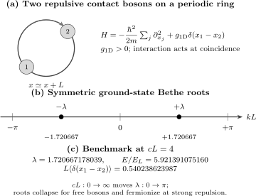
The two-boson periodic benchmark has roots $kL=\pm\lambda$. Repulsion moves them continuously from the collapsed free-boson value $\lambda=0$ toward the fermionized value $\lambda=\pi$. At $cL=4$, $\lambda=1.720667178039$ and $E/E_L=5.921391075160$.

Pair-contact derivative

Implicit differentiation of

$$F(\lambda;\alpha)=0$$

gives

$$\frac{d\lambda}{d\alpha} = \frac{ 4\lambda }{ \alpha^2 +4\lambda^2 +4\alpha }.$$

Because

$$g_{\mathrm{1D}} = \frac{\hbar^2\alpha}{mL},$$

Hellmann–Feynman implies

$$\frac{d}{d\alpha} \left( \frac E{E_L} \right) = 2L \left\langle \delta(x_1-x_2) \right\rangle.$$

Using $E/E_L=2\lambda^2$,

$$\begin{aligned} L \left\langle \delta(x_1-x_2) \right\rangle &= 2\lambda \frac{d\lambda}{d\alpha} \\ &= \frac{ 8\lambda^2 }{ \alpha^2+4\lambda^2+4\alpha }. \end{aligned}$$

At $\alpha=4$,

$$\frac{d\lambda}{d\alpha} = 0.156985217967,$$

and

$$L \left\langle \delta(x_1-x_2) \right\rangle = 0.540238623987.$$

The contact decreases toward zero as repulsion enforces impenetrability, even though the interaction coefficient itself grows.

Benchmark contract

A reproducible solver should report:

1. the physical Hamiltonian and the definition $c=mg_{\mathrm{1D}}/\hbar^2$;
2. periodic boundary conditions and fixed $N=2$;
3. quantum numbers $(-1/2,+1/2)$;
4. the logarithmic branch and root ordering;
5. $\alpha=cL=4$ and energy unit $E_L=\hbar^2/(2mL^2)$;
6. both roots, total momentum, and energy;
7. the maximum Bethe-equation residual;
8. $d\lambda/d\alpha$ and the pair-contact derivative;
9. convergence tolerances and numerical precision.

Solving only the exponential equations can admit branch ambiguity. Reporting the logarithmic quantum numbers makes the state identity reproducible.

Numerical and Analytical Methods

Finite Bethe-root solvers

Newton, trust-region, and continuation methods solve the logarithmic equations efficiently for repulsive roots. Start from a known weak- or strong-coupling branch, maintain root ordering, and monitor both residuals and the Gaudin Jacobian. Sorting roots after every iteration without tracking quantum numbers can silently change the state.

Integral-equation solvers

The ground-state and Yang–Yang equations can be discretized by quadrature and solved iteratively or by Newton methods. Report momentum cutoffs, grid refinement, tail estimates, and thermodynamic-derivative stability.

Form-factor summation

Algebraic Bethe ansatz and determinant formulas turn correlators into sums over intermediate states. Numerical completeness is assessed by spectral sum-rule saturation, not by the number of states alone.

Quantum Monte Carlo

Worldline and path-integral methods are natural for equilibrium bosons and provide independent equation-of-state and correlation checks. Contact interactions require a propagator or discretization that reproduces the cusp.

Continuum and lattice tensor methods

Continuum matrix-product states or carefully extrapolated Bose–Hubbard discretizations can address inhomogeneity and dynamics. A lattice calculation approaches Lieb–Liniger only through an explicit low-density, small-spacing, coupling-matching limit.

Weak-coupling field methods

Gross–Pitaevskii, Bogoliubov, and hydrodynamic expansions are efficient when depletion and phase fluctuations are controlled on the target scales. Their failure at large $\gamma$ is physical, not a numerical inconvenience.

Principal Variants

Attractive interaction

For

$$g_{\mathrm{1D}}\lt0,$$

Bethe roots form complex strings describing bound clusters. The attractive ground state and metastable gas-like branches have different physics from the repulsive real-root baseline. Reusing the repulsive root equations with an unrestricted sign change is not a complete treatment.

Harmonic trap

An added term

$$\sum_j \frac12m\omega^2x_j^2$$

breaks translation and standard Bethe integrability. Local-density theory can import the homogeneous equation of state when the trap varies slowly.

Quasi-one-dimensional realization

Transverse confinement generates an effective $g_{\mathrm{1D}}$ whose relation to the three-dimensional scattering length includes confinement-induced renormalization. Directly inserting the three-dimensional coupling into the one-dimensional Hamiltonian is incorrect.

Multicomponent gases

Internal spin or species labels lead to nested Bethe ansatz in selected integrable models and introduce spin–charge separation, exchange structure, and additional couplings.

Finite-range and three-body terms

Effective range, dipolar tails, three-body interactions, and loss terms add new parameters and usually break the Lieb–Liniger conserved hierarchy.

Generalized hydrodynamics

Slowly varying local rapidity distributions support a generalized hydrodynamic description of large-scale inhomogeneous dynamics. It is an emergent kinetic theory built from integrability data, not a replacement for the microscopic Hamiltonian.

Model Boundaries

• Lieb–Liniger versus ideal Bose gas: $g_{\mathrm{1D}}=0$ is a singular boundary for several thermodynamic and correlation limits.
• Lieb–Liniger versus Tonks–Girardeau: the latter is the impenetrable limit, with an additional exact Bose–Fermi mapping.
• Lieb–Liniger versus Bose–Hubbard chain: one is a continuum contact gas; the other has a lattice, band curvature, commensurability, and onsite interaction.
• Lieb–Liniger versus Luttinger liquid: the microscopic model fixes nonuniversal parameters; the Luttinger theory is its universal infrared description.
• Uniform versus trapped gas: a trap is additional model data and generally removes exact translation-invariant Bethe equations.
• Repulsive versus attractive gas: real roots and cluster strings belong to different branches and stability questions.

Common Mistakes

• Dropping the factor $1/2$ in the field interaction while keeping the same $g_{\mathrm{1D}}$.
• Confusing $c=mg_{\mathrm{1D}}/\hbar^2$ with $2c$, the coefficient inside the dimensionless first-quantized Hamiltonian.
• Treating $\alpha=cL$ and $\gamma=c/n$ as interchangeable at finite $N$.
• Forgetting whether even-$N$ Bethe quantum numbers are half odd integers.
• Solving exponential Bethe equations without reporting logarithmic branches.
• Calling rapidities ordinary free-particle momenta at finite coupling.
• Assuming bosons may repeat Bethe quantum numbers because they may repeat one-particle orbitals in the ideal gas.
• Treating exact energies as proof that every correlation function is simple.
• Applying the free-fermion mapping to bosonic one-body coherence at finite or infinite coupling.
• Calling the weak-to-strong crossover a Mott transition without a lattice.
• Using Gross–Pitaevskii theory at large $\gamma$ because the field Hamiltonian still looks local.
• Carrying a three-dimensional scattering coupling into one dimension without confinement matching.
• Calling a trapped finite cloud exactly integrable because its local equation of state comes from Bethe ansatz.
• Comparing contact values defined with different Fourier and density normalizations.

Summary

• The model describes continuum bosons with repulsive delta-function interactions on a declared one-dimensional geometry.
• $g_{\mathrm{1D}}$, $c$, $\gamma$, and $\alpha$ are related but serve different conventions and limits.
• The contact interaction is encoded by a derivative cusp.
• Periodic finite-volume eigenstates are labeled by Bethe quantum numbers and real rapidities.
• Bethe ansatz gives exact spectra and equilibrium thermodynamics, not automatically elementary correlators.
• The weak and strong limits connect mean-field Bose physics to fermionized energies through a crossover.
• The two-boson $cL=4$ benchmark fixes roots, energy, residual, and pair contact without a basis cutoff.

Exercises

1. Reconcile the coupling conventions

Starting from

$$H = -\frac{\hbar^2}{2m} \sum_j\partial_{x_j}^2 + g_{\mathrm{1D}} \sum_{j\lt\ell} \delta(x_j-x_\ell),$$

factor out $\hbar^2/(2m)$ and derive the coefficient of the delta interaction in terms of $c=mg_{\mathrm{1D}}/\hbar^2$.

Solution

Write

$$g_{\mathrm{1D}} = \frac{\hbar^2c}{m}.$$

Then

$$\begin{gathered} g_{\mathrm{1D}} \sum_{j\lt\ell}\delta(x_j-x_\ell) \\ = \frac{\hbar^2}{2m} \left[ 2c \sum_{j\lt\ell} \delta(x_j-x_\ell) \right]. \end{gathered}$$

Therefore

$$\begin{aligned} H ={}& \frac{\hbar^2}{2m} \Bigg[ -\sum_j\partial_{x_j}^2 \\ &\qquad+ 2c \sum_{j\lt\ell} \delta(x_j-x_\ell) \Bigg]. \end{aligned}$$

The coefficient is $2c$, not $c$. The separate $1/2$ in the second-quantized quartic term performs pair counting and is consistent with the same physical coupling.

2. Derive the cusp condition

For two particles, integrate the Schrödinger equation over $-\eta\lt r\lt\eta$ and take $\eta\to0^+$. Show that the relative derivative jumps by $c\Psi(0)$.

Solution

With

$$r=x_1-x_2,$$

the relative kinetic term is

$$-\frac{\hbar^2}{m} \partial_r^2.$$

Terms finite over the shrinking interval vanish. Integration leaves

$$\begin{aligned} 0 ={}& -\frac{\hbar^2}{m} \partial_r\Psi(0^+) \\ &+ \frac{\hbar^2}{m} \partial_r\Psi(0^-) \\ &+ g_{\mathrm{1D}}\Psi(0). \end{aligned}$$

Hence

$$\begin{aligned} \partial_r\Psi(0^+) - \partial_r\Psi(0^-) &= c\Psi(0), \\ c &= \frac{mg_{\mathrm{1D}}}{\hbar^2}. \end{aligned}$$

For an even bosonic relative wavefunction, the two one-sided derivatives have opposite signs, giving $2\partial_r\Psi(0^+)=c\Psi(0)$.

3. Reduce the two-boson Bethe equations

Use $I_{1,2}=\mp1/2$ and $k_{1,2}=\mp q$ to derive

$$\lambda + 2\arctan\left( \frac{2\lambda}{\alpha} \right) = \pi.$$

Solution

For the positive rapidity,

$$\begin{aligned} qL ={}& 2\pi\left(\frac12\right) \\ &- 2\arctan\left( \frac{q-(-q)}{c} \right). \end{aligned}$$

Therefore

$$qL = \pi - 2\arctan\left( \frac{2q}{c} \right).$$

Using

$$\lambda=qL, \qquad \alpha=cL,$$

gives

$$\lambda + 2\arctan\left( \frac{2\lambda}{\alpha} \right) = \pi.$$

The negative-root equation is the negative of the same relation and is automatically satisfied.

4. Check the limiting roots

Show that $\lambda\sim\sqrt{\alpha}$ for $\alpha\to0^+$ and $\lambda\to\pi$ for $\alpha\to\infty$. Find the leading strong-coupling correction.

Solution

At weak coupling, the relevant ratio $2\lambda/\alpha$ is large. Use

$$\arctan z = \frac\pi2-\frac1z+\cdots$$

for $z\gt0$. The root equation becomes

$$\lambda + \pi - \frac{\alpha}{\lambda} \simeq \pi,$$

so

$$\lambda^2 \simeq \alpha.$$

At strong coupling, $2\lambda/\alpha$ is small and

$$\arctan\left( \frac{2\lambda}{\alpha} \right) \simeq \frac{2\lambda}{\alpha}.$$

Thus

$$\lambda \left( 1+\frac4\alpha \right) \simeq \pi,$$

or

$$\lambda \simeq \pi \left( 1-\frac4\alpha \right).$$

Consequently

$$\frac E{E_L} \simeq 2\pi^2 \left( 1-\frac8\alpha \right).$$

5. Obtain the pair contact

Differentiate the root equation implicitly and derive

$$L \langle\delta(x_1-x_2)\rangle = \frac{ 8\lambda^2 }{ \alpha^2+4\lambda^2+4\alpha }.$$

Solution

For

$$F = \lambda + 2\arctan\left( \frac{2\lambda}{\alpha} \right) - \pi,$$

the partial derivatives are

$$\frac{\partial F}{\partial\lambda} = 1 + \frac{4\alpha}{ \alpha^2+4\lambda^2 },$$ $$\frac{\partial F}{\partial\alpha} = -\frac{4\lambda}{ \alpha^2+4\lambda^2 }.$$

Therefore

$$\frac{d\lambda}{d\alpha} = -\frac{\partial_\alpha F}{\partial_\lambda F} = \frac{ 4\lambda }{ \alpha^2+4\lambda^2+4\alpha }.$$

Since

$$\frac E{E_L} = 2\lambda^2,$$

Hellmann–Feynman gives

$$\begin{aligned} L \langle\delta(x_1-x_2)\rangle &= \frac12 \frac{d}{d\alpha} \left( \frac E{E_L} \right) \\ &= 2\lambda \frac{d\lambda}{d\alpha}, \end{aligned}$$

which yields the stated result.

6. Density tunes the interaction

Hold $m$ and $g_{\mathrm{1D}}$ fixed while lowering the density from $n$ to $n/5$. How does $\gamma$ change? Does this operation by itself tune the finite-ring parameter $\alpha$ if $L$ is held fixed?

Solution

Because

$$\gamma = \frac{mg_{\mathrm{1D}}}{\hbar^2n},$$

replacing $n$ by $n/5$ gives

$$\gamma' = 5\gamma.$$

The gas becomes more strongly interacting in dimensionless terms.

By contrast,

$$\alpha = \frac{mg_{\mathrm{1D}}L}{\hbar^2}$$

depends on coupling and ring length, not directly on $N$. If $L$ and $g_{\mathrm{1D}}$ are fixed, $\alpha$ is unchanged while reducing particle number changes

$$\gamma = \frac{\alpha}{N}.$$

This is why finite-size and thermodynamic coupling conventions must be reported separately.

Cross-Links

• Model Encyclopedia Overview — model-family comparisons and the Lieb–Liniger to Tonks–Girardeau relation.
• Tonks–Girardeau Gas Preview — impenetrable limit, Bose–Fermi map, ring boundary twist, and observable distinctions.
• Low-Dimensional Quantum Gases — dimensionality, confinement, ideal-gas infrared behavior, and experimental orientation.
• Nonrelativistic Field Theory from Many-Body QM — field normalization and QFT bridge.
• Luttinger Liquid Preview — infrared Hamiltonian, correlation exponents, and perturbations.
• Gross–Pitaevskii Equation — weak-coupling mean-field dynamics and failure conditions.
• Bogoliubov Theory — weakly depleted fluctuation theory.
• Exact Solutions Preview — distinctions among free modes, mappings, and Bethe ansatz.
• Integrability and Generalized Gibbs Ensembles Preview — conserved charges and relaxation.
• Quantum Quenches — nonequilibrium protocols and observable dependence.
• Common Many-Body Hamiltonians — compact continuum-boson convention lookup.

References

1. E. H. Lieb and W. Liniger, “Exact Analysis of an Interacting Bose Gas. I. The General Solution and the Ground State”, Physical Review 130, 1605–1616 (1963) — coordinate Bethe ansatz and thermodynamic ground state.
2. E. H. Lieb, “Exact Analysis of an Interacting Bose Gas. II. The Excitation Spectrum”, Physical Review 130, 1616–1624 (1963) — type-I and type-II excitation branches.
3. C. N. Yang and C. P. Yang, “Thermodynamics of a One-Dimensional System of Bosons with Repulsive Delta-Function Interaction”, Journal of Mathematical Physics 10, 1115–1122 (1969) — exact finite-temperature thermodynamics.
4. M. Girardeau, “Relationship between Systems of Impenetrable Bosons and Fermions in One Dimension”, Journal of Mathematical Physics 1, 516–523 (1960) — hard-core Bose–Fermi mapping.
5. M. Olshanii, “Atomic Scattering in the Presence of an External Confinement and a Gas of Impenetrable Bosons”, Physical Review Letters 81, 938–941 (1998) — confinement-induced one-dimensional coupling.
6. V. E. Korepin, N. M. Bogoliubov, and A. G. Izergin, Quantum Inverse Scattering Method and Correlation Functions, Cambridge University Press (1993) — algebraic Bethe ansatz, norms, and correlation structures.
7. K. V. Kheruntsyan, D. M. Gangardt, P. D. Drummond, and G. V. Shlyapnikov, “Pair Correlations in a Finite-Temperature 1D Bose Gas”, Physical Review Letters 91, 040403 (2003) — local correlations across thermal regimes.
8. J.-S. Caux and P. Calabrese, “Dynamical Density–Density Correlations in the One-Dimensional Bose Gas”, Physical Review A 74, 031605 (2006) — form-factor computation of the dynamic structure factor.
9. T. Kinoshita, T. Wenger, and D. S. Weiss, “Observation of a One-Dimensional Tonks–Girardeau Gas”, Science 305, 1125–1128 (2004) — experimental strongly correlated one-dimensional bosons.
10. A. H. van Amerongen, J. J. P. van Es, P. Wicke, K. V. Kheruntsyan, and N. J. van Druten, “Yang–Yang Thermodynamics on an Atom Chip”, Physical Review Letters 100, 090402 (2008) — experimental equation of state compared with Yang–Yang thermodynamics.