Gross–Pitaevskii Equation

The Gross–Pitaevskii equation is the leading nonlinear field equation for a dilute Bose condensate whose depletion and short-range many-body correlations are small. For a single component in three dimensions, its standard time-dependent form is

$$i\hbar\frac{\partial\Psi}{\partial t} = \left[ -\frac{\hbar^2}{2m}\nabla^2 +V_{\mathrm{ext}} +g|\Psi|^2 \right]\Psi,$$

where the condensate field is normalized here by

$$\int d^3r\,|\Psi(\mathbf r,t)|^2 = N,$$

and the leading low-energy coupling is

$$g = \frac{4\pi\hbar^2a_s}{m}.$$

Thus $|\Psi|^2$ is a number density, not a one-particle probability density. The nonlinearity is not an arbitrary modification of Schrödinger dynamics: it is the functional derivative of a mean-field interaction energy. That variational origin fixes the factor $1/2$ in the energy, the coefficient in the equation, the conserved quantities, and the relation between energy and chemical potential.

Gross–Pitaevskii theory is simultaneously simple and subtle. It can describe strongly deformed trapped profiles, sound, interference, solitons, and quantized vortices even while the gas remains microscopically dilute. But it does not include condensate depletion, thermal-cloud kinetics, generic dissipation, fragmentation, or strong correlations. Trustworthy use begins by keeping those boundaries visible.

Canonical Scope

This page is the canonical home for:

• the number-normalized and unit-normalized condensate conventions;
• the Gross–Pitaevskii energy functional and its constrained variation;
• the time-independent and time-dependent equations;
• number, energy, and current conservation within the closed theory;
• the healing length and a resolved boundary profile;
• the density–phase hydrodynamic form;
• harmonic traps, the Thomas–Fermi limit, and trap scaling;
• vortex circulation and the role of the healing-length core;
• practical validity tests, common mistakes, and numerical checks.

The statistical definition of condensation remains in Bose–Einstein Condensation. The operator Hamiltonian and ultraviolet meaning of a contact coupling belong to Field Operators in Many-Body Models, while the two-body threshold parameter belongs to Scattering Length. Weakly Interacting Bose Gas Preview owns the uniform-gas equation of state, depletion, Lee–Huang–Yang correction, and a preview of quasiparticles. Bogoliubov Theory owns the systematic fluctuation expansion and quasiparticle diagonalization.

Regime and Assumptions

The baseline theory used below assumes:

• one species of spinless bosons;
• a macroscopically occupied condensate mode;
• three spatial dimensions;
• a short-range interaction probed at low collision energy;
• a dilute gas, locally satisfying $n a_s^3\ll1$;
• small quantum and thermal depletion;
• spatial variation slow compared with the interaction range;
• a closed, conservative evolution unless explicitly stated otherwise.

The gas can still be far from ideal. In a harmonic trap, for example, the collective parameter $Na_s/a_{\mathrm{ho}}$ may be large while the local gas parameter $n a_s^3$ remains small. The first controls how much the condensate profile is reshaped by interactions; the second controls omitted correlation corrections. Confusing these parameters is a common source of contradictory claims about whether Gross–Pitaevskii theory is valid.

For the main discussion take $a_s>0$, so $g>0$ and the local interaction is repulsive. Attractive condensates require a separate stability analysis because the cubic focusing energy favors collapse.

Two Normalization Conventions

Two conventions appear throughout the literature. Both are correct, but their nonlinear coefficients differ.

Number-normalized field

The convention used on this page is

$$\int d^3r\,|\Psi|^2 = N.$$

Then $n=|\Psi|^2$ is the condensate number density and the equation contains $g|\Psi|^2$.

Unit-normalized orbital

Alternatively, write

$$\Psi(\mathbf r,t) = \sqrt N\,\phi(\mathbf r,t), \qquad \int d^3r\,|\phi|^2 = 1.$$

The large-$N$ equation becomes

$$i\hbar\partial_t\phi = \left[ -\frac{\hbar^2}{2m}\nabla^2 +V_{\mathrm{ext}} +gN|\phi|^2 \right]\phi.$$

For an exact fixed-$N$ Hartree product, pair counting gives $g(N-1)|\phi|^2$ instead of $gN|\phi|^2$. Equivalently, the number-normalized interaction energy carries a factor $1-1/N$. Standard Gross–Pitaevskii notation drops this relative $O(1/N)$ distinction. It should be restored when finite-particle counting matters.

Low-Energy Many-Body Hamiltonian

The nonrelativistic contact model is

$$\begin{aligned} \hat H ={}& \int d^3r\, \hat\psi^\dagger \left[ -\frac{\hbar^2}{2m}\nabla^2 +V_{\mathrm{ext}}(\mathbf r,t) \right] \hat\psi \\ &+ \frac{g}{2} \int d^3r\, \hat\psi^\dagger \hat\psi^\dagger \hat\psi \hat\psi. \end{aligned}$$

The fields obey

$$[\hat\psi(\mathbf r),\hat\psi^\dagger(\mathbf r')] = \delta^{(3)}(\mathbf r-\mathbf r').$$

The contact term is an effective low-energy representation. In three dimensions, matching the two-body amplitude gives

$$g = \frac{4\pi\hbar^2a_s}{m}$$

at leading order. This $g$ is expressed in terms of the physical scattering length. It is not permission to insert an unregulated delta potential into every ultraviolet-sensitive calculation. Once loop integrals, zero-point energies, or high-momentum modes are retained, the bare coupling depends on the regulator and must be matched.

The conditions

$$k|r_e| \ll 1, \qquad n a_s^3 \ll 1$$

control different approximations. The first suppresses effective-range corrections in two-body scattering; the second suppresses many-body depletion and correlation corrections. Here $r_e$ denotes the effective range and $k$ a representative relative momentum.

From the Operator Field to a Condensate Field

The exact Heisenberg equation for the contact model is

$$i\hbar\partial_t\hat\psi = \left[ -\frac{\hbar^2}{2m}\nabla^2 +V_{\mathrm{ext}} +g\hat\psi^\dagger\hat\psi \right] \hat\psi.$$

A symmetry-breaking mean-field treatment writes

$$\hat\psi = \Psi + \delta\hat\psi$$

and neglects the fluctuation terms at leading order. Equivalently, it factorizes the cubic expectation value as

$$\langle \hat\psi^\dagger\hat\psi\hat\psi \rangle \approx |\Psi|^2\Psi.$$

That replacement yields the time-dependent Gross–Pitaevskii equation. It is physically informative but not by itself a controlled error estimate. Control comes from the dilute limit, small depletion, scale separation, and the observable under study.

There is also a number-conserving route. Restrict the many-body state to a fixed-$N$ product in one orbital, evaluate the Hamiltonian, and vary the orbital. This gives the same leading equation with the finite-$N$ pair-counting correction. Hartree Approximation develops that variational connection in detail.

Gross–Pitaevskii Energy Functional

For a static external potential, define

$$\begin{aligned} E[\Psi] = \int d^3r\, \bigg[ &\frac{\hbar^2}{2m}|\boldsymbol\nabla\Psi|^2 +V_{\mathrm{ext}}|\Psi|^2 \\ &+ \frac{g}{2}|\Psi|^4 \bigg]. \end{aligned}$$

It is useful to name the three contributions:

$$E = E_{\mathrm{kin}} + E_{\mathrm{trap}} + E_{\mathrm{int}},$$

with

$$\begin{aligned} E_{\mathrm{kin}} &= \frac{\hbar^2}{2m} \int d^3r\,|\boldsymbol\nabla\Psi|^2, \\ E_{\mathrm{trap}} &= \int d^3r\,V_{\mathrm{ext}}|\Psi|^2, \\ E_{\mathrm{int}} &= \frac{g}{2} \int d^3r\,|\Psi|^4. \end{aligned}$$

The factor $1/2$ in $E_{\mathrm{int}}$ counts each pair once. Functional differentiation removes that factor because either member of a pair can be varied:

$$\frac{\delta E_{\mathrm{int}}} {\delta\Psi^*} = g|\Psi|^2\Psi.$$

The ground-state problem is therefore a constrained minimization of $E[\Psi]$ at fixed $N$, not a linear eigenvalue problem with a prescribed potential.

Time-Independent Equation

Introduce a Lagrange multiplier $\mu$ and vary

$$\mathcal F[\Phi] = E[\Phi] - \mu \left( \int d^3r\,|\Phi|^2-N \right).$$

Treat $\Phi$ and $\Phi^*$ as independent variables. The first variation with respect to $\Phi^*$ is

$$\begin{aligned} \delta\mathcal F = \int d^3r\, \bigg[ &\frac{\hbar^2}{2m} \boldsymbol\nabla(\delta\Phi^*) \boldsymbol\cdot \boldsymbol\nabla\Phi \\ &+ \left( V_{\mathrm{ext}} +g|\Phi|^2 -\mu \right) \Phi\,\delta\Phi^* \bigg]. \end{aligned}$$

After integration by parts, and assuming decay, periodicity, Dirichlet data, or another boundary condition that removes the surface term,

$$\begin{aligned} \delta\mathcal F = \int d^3r\, \delta\Phi^* \bigg[ &-\frac{\hbar^2}{2m}\nabla^2 +V_{\mathrm{ext}} \\ &+g|\Phi|^2 -\mu \bigg] \Phi. \end{aligned}$$

Stationarity for arbitrary $\delta\Phi^*$ gives

$$\left[ -\frac{\hbar^2}{2m}\nabla^2 +V_{\mathrm{ext}}(\mathbf r) +g|\Phi(\mathbf r)|^2 \right] \Phi(\mathbf r) = \mu\Phi(\mathbf r).$$

This is the time-independent Gross–Pitaevskii equation. The multiplier $\mu$ is the chemical potential associated with changing the condensate population along the family of optimized states:

$$\mu = \frac{\partial E_0}{\partial N}$$

when the derivative exists and all external parameters are fixed.

Chemical potential is not energy per particle

Multiply the stationary equation by $\Phi^*$ and integrate. One obtains

$$\mu N = E_{\mathrm{kin}} + E_{\mathrm{trap}} + 2E_{\mathrm{int}}.$$

Since

$$E = E_{\mathrm{kin}} + E_{\mathrm{trap}} + E_{\mathrm{int}},$$

the relation is

$$E = \mu N - E_{\mathrm{int}}.$$

The nonlinear eigenvalue $\mu$ therefore differs from $E/N$ whenever interactions contribute. Calling $\mu$ the energy of the condensate wavefunction obscures this distinction.

Time-Dependent Equation from an Action

The conservative dynamics follows from

$$S = \int dt\,L,$$

with

$$\begin{aligned} L = \int d^3r\, \bigg[ &\frac{i\hbar}{2} \left( \Psi^*\partial_t\Psi - \Psi\partial_t\Psi^* \right) \\ &- \frac{\hbar^2}{2m}|\boldsymbol\nabla\Psi|^2 - V_{\mathrm{ext}}|\Psi|^2 - \frac{g}{2}|\Psi|^4 \bigg]. \end{aligned}$$

Varying with respect to $\Psi^*$ gives

$$i\hbar\partial_t\Psi = \frac{\delta E}{\delta\Psi^*} = \left[ -\frac{\hbar^2}{2m}\nabla^2 +V_{\mathrm{ext}} +g|\Psi|^2 \right]\Psi.$$

For a static stationary profile,

$$\Psi(\mathbf r,t) = e^{-i\mu t/\hbar} \Phi(\mathbf r),$$

and the time-dependent equation reduces to the stationary one. A stationary density can therefore carry a uniformly rotating phase.

Conservation Laws

The time-dependent equation preserves the norm when $V_{\mathrm{ext}}$ and $g$ are real. Define

$$n = |\Psi|^2$$

and

$$\mathbf j = \frac{\hbar}{2mi} \left( \Psi^*\boldsymbol\nabla\Psi - \Psi\boldsymbol\nabla\Psi^* \right).$$

Combining the equation with its complex conjugate gives the local continuity equation

$$\partial_t n + \boldsymbol\nabla\boldsymbol\cdot\mathbf j = 0.$$

Under vanishing normal current or suitable decay,

$$\frac{dN}{dt} = 0.$$

If $V_{\mathrm{ext}}$ has no explicit time dependence, then

$$\frac{dE}{dt} = 0.$$

For a driven trap,

$$\frac{dE}{dt} = \int d^3r\, n(\mathbf r,t) \frac{\partial V_{\mathrm{ext}}}{\partial t}.$$

Thus ordinary time-dependent Gross–Pitaevskii evolution is Hamiltonian. Imaginary-time propagation, damping terms, stochastic noise, and particle-loss terms are additional models; they are not hidden inside the conservative equation.

Uniform Condensate

Set $V_{\mathrm{ext}}=0$ and consider a uniform solution

$$\Psi_0 = \sqrt{n_0} e^{-i\mu t/\hbar}.$$

The stationary equation gives

$$\mu = gn_0.$$

The leading energy density and pressure are

$$\mathcal E = \frac{g}{2}n_0^2, \qquad P = \frac{g}{2}n_0^2.$$

The inverse compressibility scale is finite:

$$\frac{\partial\mu}{\partial n_0} = g.$$

This is the simplest indication that weak repulsion changes the ideal condensate qualitatively. It costs energy to compress the density, and long-wavelength disturbances propagate as sound rather than as independent quadratic particles.

Healing Length

Suppose a repulsive uniform condensate is disturbed near a wall, defect, interface, or vortex core. The density cannot jump discontinuously because the gradient energy would diverge. It recovers over the distance at which kinetic and interaction energies balance:

$$\frac{\hbar^2}{2m\xi^2} \sim gn_0.$$

This page uses the convention

$$\xi = \frac{\hbar}{\sqrt{2mgn_0}} = \frac{1}{\sqrt{8\pi a_s n_0}}.$$

Some texts define $\xi'=\hbar/\sqrt{mgn_0}=\sqrt2\,\xi$. Formulas involving a numerical factor of $\sqrt2$ must therefore be compared only after the convention is identified.

Exact planar healing profile

Take a hard wall at $x=0$, a condensate for $x>0$, and boundary conditions

$$\Phi(0) = 0, \qquad \Phi(x\to\infty) = \sqrt{n_0}.$$

Write

$$\Phi(x) = \sqrt{n_0}\,f(x), \qquad \mu = gn_0.$$

The stationary equation becomes

$$-\xi^2 f'' + (f^2-1)f = 0.$$

Its monotone solution is

$$f(x) = \tanh \left( \frac{x}{\sqrt2\,\xi} \right),$$

so the density profile is

$$\frac{n(x)}{n_0} = \tanh^2 \left( \frac{x}{\sqrt2\,\xi} \right).$$

The healing length is not a hard cutoff. It is the scale controlling a smooth crossover. Different operational definitions, such as the half-density distance, differ by order-one constants.

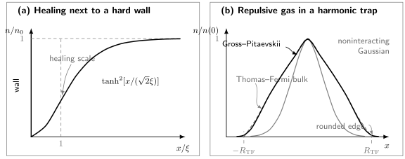
Two roles of the gradient term. Near a hard wall, the density heals as $\tanh^2[x/(\sqrt2\xi)]$. In a harmonic trap, repulsion broadens the condensate from the noninteracting Gaussian toward a Thomas–Fermi profile; the neglected gradient term remains essential in the edge layer.

Density–Phase Hydrodynamics

Where $n>0$, write the condensate field as

$$\Psi = \sqrt n\,e^{i\theta}.$$

The current becomes

$$\mathbf j = n\mathbf v, \qquad \mathbf v = \frac{\hbar}{m}\boldsymbol\nabla\theta.$$

The imaginary part of the Gross–Pitaevskii equation gives

$$\partial_t n + \boldsymbol\nabla\boldsymbol\cdot(n\mathbf v) = 0.$$

The real part gives a Bernoulli-like equation,

$$\hbar\partial_t\theta + \frac{m}{2}v^2 + V_{\mathrm{ext}} + gn + Q = 0,$$

where

$$Q = -\frac{\hbar^2}{2m} \frac{\nabla^2\sqrt n}{\sqrt n}$$

is the quantum-pressure potential. Taking a gradient gives

$$m \left( \partial_t + \mathbf v\boldsymbol\cdot\boldsymbol\nabla \right) \mathbf v = -\boldsymbol\nabla \left( V_{\mathrm{ext}} +gn +Q \right)$$

where the flow is smooth and irrotational. The name quantum pressure is conventional; $Q$ is a chemical-potential contribution generated by density gradients, not the thermodynamic pressure $P=gn^2/2$.

Long-wavelength sound

Linearize around $n=n_0$ and $\mathbf v=0$. For a plane-wave perturbation, one obtains

$$\omega^2 = c^2k^2 + \frac{\hbar^2k^4}{4m^2},$$

with

$$c = \sqrt{\frac{gn_0}{m}}.$$

For $k\xi\ll1$, the first term dominates and $\omega\approx ck$. For $k\xi\gg1$, the gradient term restores particle-like curvature. The same dispersion emerges from a Bogoliubov quasiparticle calculation, but that calculation additionally determines mode amplitudes, commutators, depletion, and zero-point corrections.

When quantum pressure may be neglected

If the density varies on a scale $L\gg\xi$, then

$$\frac{|Q|}{gn} \sim \frac{\xi^2}{L^2} \ll 1.$$

Dropping $Q$ gives classical-looking compressible, irrotational hydrodynamics. The approximation fails at edges, vortex cores, solitons, sharp barriers, and dispersive shock structures precisely because $L$ becomes comparable to $\xi$.

Harmonic Traps

Consider

$$V_{\mathrm{ext}} = \frac{m}{2} \left( \omega_x^2x^2 + \omega_y^2y^2 + \omega_z^2z^2 \right).$$

Define the geometric-mean frequency and oscillator length

$$\bar\omega = (\omega_x\omega_y\omega_z)^{1/3}, \qquad a_{\mathrm{ho}} = \sqrt{\frac{\hbar}{m\bar\omega}}.$$

For $g=0$, the condensate occupies the one-particle harmonic-oscillator ground state. Repulsion broadens the density because reducing $|\Psi|^4$ lowers the interaction energy at the price of kinetic and trapping energy.

The central trap parameter is

$$\eta = \frac{Na_s}{a_{\mathrm{ho}}}.$$

Small $\eta$ gives a profile close to the oscillator Gaussian. Large positive $\eta$ leads to the Thomas–Fermi regime, provided the gas remains locally dilute.

Thomas–Fermi Limit

When the density changes slowly over most of the cloud, neglect the kinetic term in the stationary equation. The local algebraic relation is

$$V_{\mathrm{ext}}(\mathbf r) + g n_{\mathrm{TF}}(\mathbf r) = \mu,$$

so

$$n_{\mathrm{TF}}(\mathbf r) = \frac{\mu-V_{\mathrm{ext}}(\mathbf r)}{g} \,\Theta \left( \mu-V_{\mathrm{ext}}(\mathbf r) \right).$$

The Heaviside factor restricts the cloud to the region $V_{\mathrm{ext}}<\mu$. For a harmonic trap, the boundary is an ellipsoid with radii

$$R_i = \sqrt{\frac{2\mu}{m\omega_i^2}}.$$

Normalization gives

$$\mu_{\mathrm{TF}} = \frac{\hbar\bar\omega}{2} \left( 15\frac{Na_s}{a_{\mathrm{ho}}} \right)^{2/5}.$$

For an isotropic trap with frequency $\omega$,

$$R_{\mathrm{TF}} = a_{\mathrm{ho}} \left( 15\frac{Na_s}{a_{\mathrm{ho}}} \right)^{1/5}.$$

At the trap center,

$$\xi(0) = \frac{\hbar}{\sqrt{2m\mu}} = \frac{a_{\mathrm{ho}}^2}{R_{\mathrm{TF}}}.$$

Thus $R_{\mathrm{TF}}\gg a_{\mathrm{ho}}$ implies $\xi(0)\ll R_{\mathrm{TF}}$, which explains why the gradient term is negligible in the bulk.

The sharp edge is an artifact

The Thomas–Fermi profile has a nonanalytic edge. The exact Gross–Pitaevskii solution rounds that edge because the density-gradient scale becomes short and quantum pressure can no longer be neglected. Thomas–Fermi theory is a bulk approximation, not a boundary condition.

Thomas–Fermi energies

For a three-dimensional harmonic trap in the Thomas–Fermi limit,

$$E_{\mathrm{trap}} = \frac{3}{7}N\mu, \qquad E_{\mathrm{int}} = \frac{2}{7}N\mu,$$

and therefore

$$E = \frac{5}{7}N\mu.$$

The result is consistent with both

$$\mu N = E_{\mathrm{trap}} + 2E_{\mathrm{int}}$$

and the harmonic-trap virial theorem.

Virial Theorem

For an isotropic or anisotropic harmonic trap, scale a normalized field as

$$\Phi_\lambda(\mathbf r) = \lambda^{3/2} \Phi(\lambda\mathbf r).$$

The three energy terms transform as

$$E_{\mathrm{kin}}(\lambda) = \lambda^2E_{\mathrm{kin}},$$ $$E_{\mathrm{trap}}(\lambda) = \lambda^{-2}E_{\mathrm{trap}},$$

and

$$E_{\mathrm{int}}(\lambda) = \lambda^3E_{\mathrm{int}}.$$

Stationarity at $\lambda=1$ gives

$$2E_{\mathrm{kin}} - 2E_{\mathrm{trap}} + 3E_{\mathrm{int}} = 0.$$

This identity is both a physical result and a powerful numerical diagnostic. A converged stationary solver can satisfy the discretized equation while still having appreciable finite-box or resolution error; the virial residual exposes many such failures.

Gaussian Variational Crossover

A simple trial profile connects the noninteracting and interaction-broadened regimes. In an isotropic trap, take

$$\Phi_\sigma(\mathbf r) = \frac{\sqrt N} {\pi^{3/4}\sigma^{3/2}} \exp \left( -\frac{r^2}{2\sigma^2} \right).$$

Its energy per particle is

$$\frac{E(\sigma)}{N\hbar\omega} = \frac{3}{4} \left( s^2 + s^{-2} \right) + \frac{Na_s/a_{\mathrm{ho}}} {\sqrt{2\pi}\,s^3},$$

where

$$s = \frac{\sigma}{a_{\mathrm{ho}}}.$$

At $a_s=0$, the minimum is $s=1$. Repulsion shifts it to $s>1$. Attraction shifts it to $s<1$ and eventually removes the local minimum. The Gaussian is not quantitatively exact in the Thomas–Fermi regime, but it makes the competition among kinetic, trap, and interaction energies transparent.

Dimensionless Form

For an isotropic harmonic trap, set

$$\mathbf r = a_{\mathrm{ho}}\mathbf x, \qquad t = \frac{\tau}{\omega}, \qquad \Psi = \frac{\sqrt N}{a_{\mathrm{ho}}^{3/2}} \psi.$$

Then

$$\int d^3x\,|\psi|^2 = 1$$

and the equation becomes

$$i\partial_\tau\psi = \left[ -\frac{1}{2}\nabla_{\mathbf x}^2 + \frac{x^2}{2} + 4\pi\frac{Na_s}{a_{\mathrm{ho}}}|\psi|^2 \right]\psi.$$

This scaling shows that the zero-temperature, one-component, isotropic contact problem has one dimensionless interaction parameter. Anisotropy introduces frequency ratios. Lower-dimensional reductions introduce different effective couplings and should not inherit the three-dimensional value of $g$ unchanged.

Quantized Vortices

The phase representation implies irrotational flow wherever $\Psi\ne0$:

$$\boldsymbol\nabla\times\mathbf v = 0.$$

Nevertheless, the phase may wind around a line where the density vanishes. Single-valuedness requires

$$\Delta\theta = 2\pi\ell, \qquad \ell\in\mathbb Z.$$

Therefore the circulation is quantized:

$$\oint\mathbf v\boldsymbol\cdot d\boldsymbol\ell = \frac{2\pi\hbar}{m}\ell.$$

For a straight vortex along $z$, an axisymmetric ansatz is

$$\Phi(\rho,\varphi,z) = f(\rho,z)e^{i\ell\varphi}.$$

The kinetic energy contains

$$\frac{\hbar^2\ell^2}{2m\rho^2}|f|^2.$$

Finite energy forces $f\to0$ on the axis, creating a core whose radius is of order the local healing length. Gross and Pitaevskii introduced their equations in precisely this vortex context. In a nonrotating simply connected trap, a vortex is generally not the ground state. In a frame rotating with angular velocity $\Omega$, the relevant functional is $E-\Omega\langle L_z\rangle$, and vortices can become energetically favorable.

Nonlinear Superposition and Stationary States

The stationary equation resembles an eigenvalue equation, but it is nonlinear. If $\Phi_1$ and $\Phi_2$ are solutions, then

$$c_1\Phi_1+c_2\Phi_2$$

is not generally a solution. Orthogonality and spectral decomposition therefore do not transfer unchanged from linear quantum mechanics.

A stationary solution can be:

• the constrained energy minimum;
• a local minimum representing a metastable state;
• a saddle such as a soliton or vortex configuration;
• dynamically unstable even though the stationary residual vanishes.

Energetic and dynamical stability are determined by the second variation and the linearized time-dependent equation. The resulting coupled mode problem is the Bogoliubov–de Gennes system, not the original stationary equation applied independently to one perturbation amplitude.

Condensate Field and Number Conservation

In a symmetry-breaking description,

$$\Psi(\mathbf r,t) = \langle\hat\psi(\mathbf r,t)\rangle.$$

But an exact eigenstate of total particle number satisfies

$$\langle\hat\psi\rangle = 0$$

because $\hat\psi$ changes the number sector. This does not mean that a fixed-$N$ condensate has no Gross–Pitaevskii description. Its condensate orbital can be defined as the dominant eigenvector of the one-body density matrix, or obtained through a number-conserving expansion. The complex phase then represents a relative phase, a symmetry-broken thermodynamic description, or a convenient representative of the condensate mode.

Observable quantities such as $n$, $\mathbf j$, phase differences, and interference signals are invariant under the global transformation

$$\Psi \longmapsto e^{i\alpha}\Psi.$$

The equation respects this global U(1) symmetry and conserves the associated norm.

Time-Dependent Uses

The conservative equation is widely used for:

• collective oscillations after a weak trap perturbation;
• expansion after release from a trap;
• phase imprinting and interference;
• flow past barriers and weak links;
• vortex nucleation and motion when the mean-field description remains valid;
• soliton and dispersive-wave dynamics;
• coherent splitting, transport, and recombination protocols.

The equation does not guarantee accuracy merely because a numerical solution exists. Rapid driving can populate noncondensed modes, produce fragmentation, or transfer weight to momenta outside the contact model’s low-energy range. The relevant validity test concerns the evolving state, not only the initial state.

Center-of-mass motion

For a harmonic trap and translation-invariant two-body interactions, the condensate center of mass obeys

$$\ddot R_i + \omega_i^2R_i = 0.$$

The contact nonlinearity does not shift this dipole frequency because internal forces cancel. This is the mean-field manifestation of center-of-mass decoupling and provides another stringent simulation check.

Practical Ground-State Workflow

A defensible Gross–Pitaevskii calculation should record:

1. the normalization convention and particle number;
2. the spatial dimension and effective coupling;
3. trap frequencies, boundary conditions, and energy units;
4. the gas parameter and effective-range estimate in the dense region;
5. the smallest expected healing length;
6. grid spacing and box size relative to physical scales;
7. convergence of norm, energy, and stationary residual;
8. a virial or analytically known limiting check.

Ground states are often found by normalized gradient flow or imaginary-time propagation. Formally setting $t=-i\tau$ damps high-energy components, but the resulting evolution does not conserve norm, so the field must be renormalized or the constraint enforced continuously. Imaginary time is an optimization algorithm, not physical condensate dynamics.

For real-time propagation, useful checks include:

• norm conservation;
• energy conservation for a static trap;
• reversibility under time-step refinement;
• the center-of-mass dipole frequency in a harmonic trap;
• convergence when the grid resolves the healing length and any vortex core;
• negligible density at artificial box boundaries when open space is intended.

Detailed discretization algorithms belong in Computational QM; these checks belong to the physical definition of a trustworthy result.

Validity and Limitations

Diluteness and depletion

For a uniform three-dimensional gas at zero temperature, the leading depletion fraction scales as

$$\frac{N-N_0}{N} \sim \sqrt{n a_s^3}.$$

Gross–Pitaevskii theory retains the leading mean field but omits this depletion and the associated Lee–Huang–Yang correction. Small $n a_s^3$ is therefore central to its ordinary dilute-gas use.

Contact matching

The formula $g=4\pi\hbar^2a_s/m$ is three-dimensional and low energy. In one or two dimensions, and in strongly confined quasi-low-dimensional geometries, the effective coupling has different dimensional dependence and may be modified by confinement-induced resonances. See Low-Dimensional Quantum Gases for the dimensional boundary.

Finite temperature

At nonzero temperature, a thermal cloud can alter the mean field, damp collective modes, exchange particles with the condensate, and generate noise. A single conservative field does not describe those processes. Finite-temperature mean-field, kinetic, stochastic, or open-system methods require additional assumptions.

Attractive interactions

For $g<0$, the three-dimensional cubic interaction lowers the energy as the density concentrates. A trap can support a metastable condensate only below a geometry-dependent critical population. Beyond it, the simple energy functional has no stable local minimum against collapse. Three-body loss and short-distance physics then become important before a mathematical singularity should be interpreted literally.

Strong correlations and fragmentation

One condensate field is inadequate for Mott phases, Tonks–Girardeau gases, strongly depleted fluids, fragmented condensates, and states whose one-body density matrix has several macroscopic eigenvalues. A large occupation number alone does not prove that connected correlations are negligible.

Long-range or internal-state interactions

Dipolar, spinor, multicomponent, spin–orbit-coupled, and cavity-mediated condensates require nonlocal kernels, coupled fields, matrix-valued order parameters, or additional dynamical variables. Calling all of these extensions Gross–Pitaevskii equations can be convenient, but their couplings and stability criteria are model specific.

Dissipation and loss

Terms such as

$$-i\hbar\frac{K_3}{2}|\Psi|^4\Psi$$

are sometimes added phenomenologically to represent three-body loss. Damped or stochastic variants are also common. Such equations no longer follow from the closed conservative action above, and their noise, damping, and fluctuation relations must be justified separately.

Rigorous limit versus informal derivation

The replacement $\hat\psi\to\Psi$ is a useful heuristic, but rigorous Gross–Pitaevskii limits retain short-range pair correlations needed to replace a microscopic potential by its scattering length. A naive uncorrelated product using the bare potential generally produces the Born integral of that potential, not automatically $4\pi\hbar^2a_s/m$. The final mean-field equation can be asymptotically correct even though the exact many-body wavefunction is not an uncorrelated product at microscopic separations.

Common Mistakes

Mixing normalization conventions

Writing $\int|\Psi|^2=1$ while also using $g|\Psi|^2$ omits the factor of $N$. State the convention before interpreting any density or coupling.

Forgetting pair counting

The interaction energy is $g|\Psi|^4/2$, while the equation contains $g|\Psi|^2$. Replacing the energy coefficient by $g$ double counts pairs.

Treating the chemical potential as total energy per particle

For an interacting stationary state, $\mu N=E+E_{\mathrm{int}}$. The nonlinear eigenvalue is an addition derivative, not generally $E/N$.

Using the three-dimensional coupling in every dimension

The expression $4\pi\hbar^2a_s/m$ is not a universal one-, two-, and three-dimensional formula.

Calling the Thomas–Fermi edge exact

The kinetic term is small in the bulk but essential near the edge. A sharp cutoff is an artifact of the approximation.

Dropping quantum pressure at a vortex core

The hydrodynamic approximation fails precisely where the density vanishes and the phase gradient is largest.

Equating numerical convergence with physical validity

A tiny residual only proves that the chosen equation was solved. It does not test depletion, effective-range corrections, thermal effects, or fragmentation.

Adding damping without changing the interpretation

A phenomenologically damped equation does not conserve the same energy and is not the closed time-dependent Gross–Pitaevskii theory.

Assuming stationary means stable

Excited nonlinear stationary solutions can be saddles or dynamically unstable. Stability requires analyzing fluctuations.

Exercises

Constrained functional variation

Starting from

$$E[\Phi] = \int d^3r\, \left[ \frac{\hbar^2}{2m}|\nabla\Phi|^2 +V|\Phi|^2 +\frac{g}{2}|\Phi|^4 \right],$$

derive the stationary Gross–Pitaevskii equation at fixed $N$. State the boundary assumption used in the kinetic term.

Solution

Vary

$$\mathcal F = E - \mu \int d^3r\,|\Phi|^2.$$

The variation with respect to $\Phi^*$ is

$$\begin{aligned} \delta\mathcal F = \int d^3r\, \bigg[ &\frac{\hbar^2}{2m} \nabla(\delta\Phi^*)\boldsymbol\cdot\nabla\Phi \\ &+ (V+g|\Phi|^2-\mu) \Phi\,\delta\Phi^* \bigg]. \end{aligned}$$

Integrating the first term by parts gives a surface term

$$\frac{\hbar^2}{2m} \int_{\partial\Omega}dS\, \delta\Phi^*\, \hat{\mathbf n}\boldsymbol\cdot\nabla\Phi.$$

It vanishes for sufficient decay, periodic boundaries, fixed Dirichlet data, or an appropriate natural boundary condition. The bulk coefficient of arbitrary $\delta\Phi^*$ must vanish:

$$\left[ -\frac{\hbar^2}{2m}\nabla^2 +V +g|\Phi|^2 \right]\Phi = \mu\Phi.$$

Chemical potential and energy

For a stationary solution, prove

$$\mu N = E_{\mathrm{kin}} +E_{\mathrm{trap}} +2E_{\mathrm{int}}.$$

Then specialize to a uniform condensate and compare $E/N$ with $\mu$.

Solution

Multiply the stationary equation by $\Phi^*$, integrate, and integrate the kinetic term by parts:

$$\begin{aligned} \mu N ={}& \frac{\hbar^2}{2m} \int d^3r\,|\nabla\Phi|^2 \\ &+ \int d^3r\,V|\Phi|^2 + g\int d^3r\,|\Phi|^4. \end{aligned}$$

The last integral is $2E_{\mathrm{int}}$, proving the identity. For a uniform gas of density $n=N/V$,

$$E = \frac{g}{2}n^2V, \qquad \frac{E}{N} = \frac{gn}{2},$$

whereas

$$\mu = gn.$$

The chemical potential is twice the interaction energy per particle in this leading uniform mean field.

Healing at a hard wall

For the dimensionless boundary equation

$$-\xi^2f'' + (f^2-1)f = 0,$$

with $f(0)=0$ and $f(\infty)=1$, derive a first integral and obtain the healing profile.

Solution

Multiply by $f'$:

$$-\xi^2f''f' + (f^2-1)ff' = 0.$$

Integrating once gives

$$-\frac{\xi^2}{2}(f')^2 + \frac{1}{4}(f^2-1)^2 = C.$$

The bulk conditions $f\to1$ and $f'\to0$ imply $C=0$. For the increasing solution,

$$f' = \frac{1-f^2}{\sqrt2\,\xi}.$$

Separating variables yields

$$\operatorname{artanh}f = \frac{x}{\sqrt2\,\xi},$$

and therefore

$$f(x) = \tanh \left( \frac{x}{\sqrt2\,\xi} \right).$$

Hydrodynamic linearization

Linearize the density–phase equations around a uniform condensate and show that

$$\omega^2 = \frac{gn_0}{m}k^2 + \frac{\hbar^2}{4m^2}k^4.$$

Identify the long-wavelength sound speed.

Solution

Write

$$n = n_0+\delta n, \qquad \mathbf v = \delta\mathbf v.$$

To linear order, continuity gives

$$\partial_t\delta n + n_0\nabla\boldsymbol\cdot\delta\mathbf v = 0.$$

Expanding the quantum-pressure potential gives

$$\delta Q = -\frac{\hbar^2}{4mn_0} \nabla^2\delta n.$$

The Euler equation becomes

$$m\partial_t\delta\mathbf v = -\nabla \left( g\delta n - \frac{\hbar^2}{4mn_0} \nabla^2\delta n \right).$$

Differentiate continuity in time and substitute the divergence of this equation:

$$\partial_t^2\delta n = \frac{gn_0}{m}\nabla^2\delta n - \frac{\hbar^2}{4m^2}\nabla^4\delta n.$$

For $e^{i(\mathbf k\cdot\mathbf r-\omega t)}$, this gives the stated dispersion. The sound speed is

$$c = \sqrt{\frac{gn_0}{m}}.$$

Isotropic Thomas–Fermi cloud

For

$$V(r) = \frac{1}{2}m\omega^2r^2,$$

normalize the Thomas–Fermi density and derive $R_{\mathrm{TF}}$ and $\mu_{\mathrm{TF}}$.

Solution

Inside the cloud,

$$n(r) = \frac{1}{g} \left( \mu - \frac{1}{2}m\omega^2r^2 \right),$$

and $n(R)=0$ gives

$$\mu = \frac{1}{2}m\omega^2R^2.$$

Normalization yields

$$\begin{aligned} N &= \frac{4\pi}{g} \int_0^Rdr\,r^2 \left( \mu-\frac{1}{2}m\omega^2r^2 \right) \\ &= \frac{4\pi m\omega^2R^5}{15g}. \end{aligned}$$

Using

$$g = \frac{4\pi\hbar^2a_s}{m}, \qquad a_{\mathrm{ho}}^2 = \frac{\hbar}{m\omega},$$

gives

$$R^5 = 15Na_s a_{\mathrm{ho}}^4.$$

Therefore

$$R_{\mathrm{TF}} = a_{\mathrm{ho}} \left( 15\frac{Na_s}{a_{\mathrm{ho}}} \right)^{1/5},$$

and

$$\mu_{\mathrm{TF}} = \frac{\hbar\omega}{2} \left( 15\frac{Na_s}{a_{\mathrm{ho}}} \right)^{2/5}.$$

Virial check

Use the norm-preserving scale transformation $\Phi_\lambda=\lambda^{3/2}\Phi(\lambda\mathbf r)$ to derive the virial theorem. Then recover the ratio of trap and interaction energies in the Thomas–Fermi limit.

Solution

Under the scale transformation,

$$E(\lambda) = \lambda^2E_{\mathrm{kin}} + \lambda^{-2}E_{\mathrm{trap}} + \lambda^3E_{\mathrm{int}}.$$

Stationarity requires

$$0 = \left. \frac{dE}{d\lambda} \right|_{\lambda=1} = 2E_{\mathrm{kin}} -2E_{\mathrm{trap}} +3E_{\mathrm{int}}.$$

In the Thomas–Fermi limit $E_{\mathrm{kin}}$ is negligible, so

$$2E_{\mathrm{trap}} = 3E_{\mathrm{int}}.$$

Together with

$$\mu N = E_{\mathrm{trap}} +2E_{\mathrm{int}},$$

this gives

$$E_{\mathrm{int}} = \frac{2}{7}N\mu, \qquad E_{\mathrm{trap}} = \frac{3}{7}N\mu.$$

Vortex circulation

Let $\Phi=f(\rho,z)e^{i\ell\varphi}$. Derive the velocity field and circulation. Explain why the density must vanish on the axis for $\ell\ne0$.

Solution

The phase is $\theta=\ell\varphi$, so

$$\mathbf v = \frac{\hbar}{m}\nabla\theta = \frac{\hbar\ell}{m\rho} \hat{\boldsymbol\varphi}.$$

Around a circle of radius $\rho$,

$$\oint\mathbf v\boldsymbol\cdot d\boldsymbol\ell = 2\pi\rho \frac{\hbar\ell}{m\rho} = \frac{2\pi\hbar\ell}{m}.$$

The phase is undefined on the axis. Moreover, the angular kinetic-energy density contains

$$\frac{\hbar^2\ell^2}{2m\rho^2}|f|^2.$$

Its transverse integral would diverge at $\rho=0$ unless $f$ vanishes sufficiently rapidly. The density therefore forms a vortex core.

Attractive Gaussian threshold

For $a_s<0$, use the Gaussian energy

$$\frac{E}{N\hbar\omega} = \frac{3}{4} \left( s^2+s^{-2} \right) - \frac{k}{\sqrt{2\pi}\,s^3},$$

where $k=N|a_s|/a_{\mathrm{ho}}$. Find the value at which the local minimum disappears.

Solution

Stationarity gives

$$s^5 -s + \frac{2k}{\sqrt{2\pi}} = 0.$$

At the disappearance of the minimum, the stationary equation has a double root. Differentiating its left side gives

$$5s^4-1 = 0,$$

so

$$s_c = 5^{-1/4}.$$

Substitution yields

$$k_c = \frac{2\sqrt{2\pi}}{5} 5^{-1/4} \approx 0.67.$$

This is a Gaussian variational estimate, not a universal exact threshold. More accurate stationary solutions give a different numerical value, and anisotropy changes it further.

Key Takeaways

• The Gross–Pitaevskii equation is the Euler–Lagrange equation of a constrained condensate energy functional.
• The number-normalized field has density $|\Psi|^2$ and nonlinearity $g|\Psi|^2$.
• In three dimensions, $g=4\pi\hbar^2a_s/m$ is a matched low-energy coupling, not an unregulated microscopic identity.
• The stationary multiplier $\mu$ is a chemical potential and generally differs from $E/N$.
• The healing length compares gradient and interaction energies and controls walls, edges, solitons, and vortex cores.
• The density–phase form becomes compressible irrotational hydrodynamics when quantum pressure is negligible.
• Repulsion broadens trapped condensates; at large $Na_s/a_{\mathrm{ho}}$, the bulk approaches the Thomas–Fermi profile.
• Small local depletion and scale separation, not mere numerical convergence, determine physical validity.

Cross-Links

• Bose–Einstein Condensation — canonical condensation criteria, critical temperatures, dimensionality, and condensate fractions.
• Bose–Einstein Condensates Overview — AMO-facing use of the field equation in density, expansion, mode, coherence, and evidence audits.
• Weakly Interacting Bose Gas Preview — uniform equation of state, depletion, Lee–Huang–Yang correction, and Bogoliubov spectrum preview.
• Field Operators in Many-Body Models — operator contact Hamiltonian, commutators, and regularization cautions.
• Density Operators and Current Operators — canonical current and continuity-equation conventions.
• Hartree Approximation — fixed-$N$ product variation and the finite-particle pair-counting factor.
• Mean-Field Theory — general self-consistency, saddle-point, and stability logic.
• Quantum Gases in Traps — ideal trapped gases, local-density methods, and trap scales.
• Chemical Potential — thermodynamic, variational, and addition-energy meanings of $\mu$.
• Scattering Length — the low-energy two-body parameter entering $g$.
• Bose–Hubbard Model — lattice projection and the boundary of a one-field continuum description.
• AMO Model Index — a decision table comparing continuum condensate, lattice, trapping, and light–matter reductions.

References

1. E. P. Gross, “Structure of a Quantized Vortex in Boson Systems,” Il Nuovo Cimento 20, 454–477 (1961), doi:10.1007/BF02731494.
2. L. P. Pitaevskii, “Vortex Lines in an Imperfect Bose Gas,” Soviet Physics JETP 13, 451–454 (1961), official JETP text.
3. F. Dalfovo, S. Giorgini, L. P. Pitaevskii, and S. Stringari, “Theory of Bose–Einstein Condensation in Trapped Gases,” Reviews of Modern Physics 71, 463–512 (1999), doi:10.1103/RevModPhys.71.463.
4. A. J. Leggett, “Bose–Einstein Condensation in the Alkali Gases: Some Fundamental Concepts,” Reviews of Modern Physics 73, 307–356 (2001), doi:10.1103/RevModPhys.73.307.
5. E. H. Lieb, R. Seiringer, and J. Yngvason, “Bosons in a Trap: A Rigorous Derivation of the Gross–Pitaevskii Energy Functional,” Physical Review A 61, 043602 (2000), doi:10.1103/PhysRevA.61.043602.
6. C. J. Pethick and H. Smith, Bose–Einstein Condensation in Dilute Gases, 2nd ed. (Cambridge University Press, 2008), doi:10.1017/CBO9780511802850.
7. L. Pitaevskii and S. Stringari, Bose–Einstein Condensation and Superfluidity (Oxford University Press, 2016), doi:10.1093/acprof:oso/9780198758884.001.0001.
8. A. L. Fetter, “Rotating Trapped Bose–Einstein Condensates,” Reviews of Modern Physics 81, 647–691 (2009), doi:10.1103/RevModPhys.81.647.
9. P. A. Ruprecht, M. J. Holland, K. Burnett, and M. Edwards, “Time-Dependent Solution of the Nonlinear Schrödinger Equation for Bose-Condensed Trapped Neutral Atoms,” Physical Review A 51, 4704–4711 (1995), doi:10.1103/PhysRevA.51.4704.
10. W. Bao and Y. Cai, “Mathematical Theory and Numerical Methods for Bose–Einstein Condensation,” Kinetic and Related Models 6, 1–135 (2013), doi:10.3934/krm.2013.6.1.