Perturbation Theory in Many-Body Systems

Many-body perturbation theory expands an interacting energy, state, free energy, response, or effective operator around a solvable many-body reference. The algebra begins with the familiar split

$$H(\lambda) = H_0+\lambda V,$$

but the many-body setting changes what must be controlled:

• the reference is itself a many-particle state or ensemble;
• one interaction connects whole families of particle–hole or occupation-number excitations;
• exact or asymptotic degeneracies proliferate with system size;
• the number of intermediate states grows with volume;
• disconnected terms must cancel from intensive quantities;
• gapless modes can make the effective expansion parameter scale or energy dependent;
• the thermodynamic limit can be nonanalytic even when every finite system is analytic.

The small parameter is therefore not merely a bare coupling $\lambda$. It is the coupling multiplied by the relevant density of states, phase space, matrix-element scale, logarithm, and inverse energy denominator.

A useful summary is

$$\text{weak microscopic interaction} \not\Longrightarrow \text{uniformly small many-body correction}.$$

The reference, observable, regulator, volume, and order of limits decide whether the expansion is meaningful.

Canonical Scope

This page is the canonical home for:

• constructing perturbation theory around a finite-volume many-body reference;
• occupied, unoccupied, particle, hole, and excitation-rank notation;
• how one- and two-body residual interactions connect reference determinants;
• the generic second-order energy in one-particle–one-hole and two-particle–two-hole sectors;
• volume counting for a translation-invariant Fermi system;
• why exact and near degeneracy are common in many-body spectra;
• linked-cluster and cumulant intuition for extensive energies and free energies;
• the distinction between energy, wavefunction, overlap, and local-observable expansions;
• finite-size, thermodynamic-limit, infrared, and ultraviolet caveats;
• diagnostic examples involving the Cooper channel, Coulomb screening, and orthogonality;
• a workflow for deciding whether to continue, change the reference, use a model space, or resum a singular channel.

Neighboring pages retain separate ownership:

• Rayleigh–Schrödinger Perturbation Theory owns the general coefficient recursion, normalization convention, and spectral-branch formulation.
• Degenerate Perturbation Theory and Quasi-Degenerate Perturbation Theory own model-space diagonalization and effective operators for a small cluster of levels.
• Normal Ordering in Many-Body QM owns the exact reference-state decomposition into zero-, one-, and residual many-body terms.
• Wick’s Theorem Preview owns Gaussian contraction rules.
• Higher-Order Structure owns the general recursion, subtraction terms, and elementary linked-cluster motivation.
• Diagrammatic Methods Preview owns Goldstone and Feynman diagram notation, propagators, vertices, self-energies, bubbles, and symmetry factors.
• Effective Hamiltonians in Many-Body Systems owns projected low-energy sectors, the many-body use of Schrieffer–Wolff elimination, and the Hubbard-to-Heisenberg and Anderson-to-Kondo maps.
• Particle–Hole Excitations owns continuum kinematics, response, hole quantum numbers, and the canonical excitation concept. This page uses those states only as perturbative intermediates.
• BCS Mean-Field Theory owns the Cooper problem and pairing saddle; Random Phase Approximation owns ring and bubble resummations in response.

The goal here is not to reproduce ordinary perturbation theory with more indices. It is to expose which many-body structures preserve or destroy the ordinary expansion.

Start with a Regulated Finite System

The cleanest order of work is:

1. choose a finite volume $\mathcal V=L^d$;
2. impose boundary conditions and a one-particle basis;
3. fix a particle-number or grand-canonical sector;
4. regulate any continuum ultraviolet behavior;
5. solve the finite reference problem;
6. construct perturbative coefficients;
7. organize connected and extensive terms;
8. only then study $L\to\infty$ and removal of the regulator.

At finite volume, a self-adjoint Hamiltonian in a finite basis is a matrix. If the chosen eigenvalue is isolated, standard analytic perturbation theory applies within a nonzero neighborhood of $\lambda=0$. The many-body difficulty is that this neighborhood may shrink with volume, the basis cutoff, or proximity to a phase transition.

Why finite volume is not a mere convenience

In a periodic box,

$$\mathbf k = \frac{2\pi}{L} \mathbf n, \qquad \mathbf n\in\mathbb Z^d.$$

Momentum sums are discrete, shell degeneracies can be identified, and every denominator has a definite value. In the thermodynamic limit the momentum spacing vanishes, sums become integrals, and arbitrarily low-energy excitations may appear.

A divergence that is invisible when one writes an integral from the start can often be diagnosed by how a finite-size coefficient scales with $L$.

Choosing the Reference Hamiltonian

A useful reference Hamiltonian is solvable and already contains the dominant one-body or quasiparticle structure. For a fermionic determinant reference, a common form is

$$H_0 = E_{\mathrm{ref}} + \sum_p \epsilon_p \{a_p^\dagger a_p\}_{\Phi},$$

where $\{\cdots\}_{\Phi}$ denotes normal ordering relative to the reference determinant $\lvert\Phi\rangle$.

The reference obeys

$$H_0\lvert\Phi\rangle = E_{\mathrm{ref}} \lvert\Phi\rangle.$$

The perturbation can contain off-diagonal one-body terms and a residual two-body interaction:

$$\begin{aligned} V &= \sum_{p,q} u_{pq} \{a_p^\dagger a_q\}_{\Phi} \\ &\quad + \frac14 \sum_{p,q,r,s} \overline v_{pq;rs} \{ a_p^\dagger a_q^\dagger a_s a_r \}_{\Phi}. \end{aligned}$$

The factor $1/4$ accompanies unrestricted sums with fully antisymmetrized two-body matrix elements. If ordered pairs are used instead, the prefactor changes.

The split is not unique

One may choose $H_0$ as:

• the noninteracting band Hamiltonian;
• a Hartree or Hartree–Fock mean field;
• a Bogoliubov quasiparticle Hamiltonian;
• a local interacting Hamiltonian in a strong-coupling expansion;
• a symmetry-preserving finite-volume reference;
• a symmetry-broken bulk representative with explicit source and limit prescription.

Different splits have the same exact endpoint $H(1)$ but different coefficients, denominators, and convergence properties.

Counterterms and double counting

If $H_0$ contains a mean field derived from the interaction, then $V$ must subtract that same mean field. Otherwise selected interaction contributions are counted once in $H_0$ and again in the perturbation.

Writing

$$H = \left( H_{\mathrm{free}}+U_{\mathrm{mf}} \right) + \left( H_{\mathrm{int}}-U_{\mathrm{mf}} \right)$$

is an exact repartitioning. Dropping the subtraction term is not.

Reference quality is observable dependent

A Hartree–Fock determinant can give a useful energy reference but a poor starting point for a pairing instability. A number-conserving Fermi sea can be ideal for normal-state response yet singular in the Cooper channel. A broken-symmetry reference can regularize one infrared problem while obscuring finite-volume symmetry restoration.

There is no reference that is uniformly optimal for every observable and scale.

Particle and Hole Intermediates

Let $i,j,k,\ldots$ label orbitals occupied in $\lvert\Phi\rangle$ and $a,b,c,\ldots$ label unoccupied orbitals. A one-particle–one-hole excitation is

$$\lvert\Phi_i^a\rangle = a_a^\dagger a_i \lvert\Phi\rangle.$$

A two-particle–two-hole excitation is

$$\lvert\Phi_{ij}^{ab}\rangle = a_a^\dagger a_b^\dagger a_j a_i \lvert\Phi\rangle.$$

For diagonal $H_0$,

$$\begin{aligned} H_0\lvert\Phi_i^a\rangle &= \left( E_{\mathrm{ref}} -\epsilon_i+\epsilon_a \right) \lvert\Phi_i^a\rangle, \\ H_0\lvert\Phi_{ij}^{ab}\rangle &= \left( E_{\mathrm{ref}} -\epsilon_i-\epsilon_j +\epsilon_a+\epsilon_b \right) \lvert\Phi_{ij}^{ab}\rangle. \end{aligned}$$

The corresponding reference-to-intermediate denominators are

$$\begin{aligned} \Delta_i^a &= \epsilon_i-\epsilon_a, \\ \Delta_{ij}^{ab} &= \epsilon_i+\epsilon_j -\epsilon_a-\epsilon_b. \end{aligned}$$

For a stable independent-particle filling, both are negative.

The corresponding upward excitation costs are positive:

$$\omega_i^a = -\Delta_i^a = \epsilon_a-\epsilon_i >0,$$

and similarly for a stable two-pair excitation.

Excitation rank is a selection rule

A normal-ordered one-body residual acting on $\lvert\Phi\rangle$ creates at most one particle–hole pair. A normal-ordered two-body residual creates at most two. Therefore:

$$\langle\Phi_i^a|V|\Phi\rangle = u_{ai},$$

and

$$\langle\Phi_{ij}^{ab}|V|\Phi\rangle = \overline v_{ab;ij},$$

with signs fixed by the determinant convention.

A generic two-body Hamiltonian written before reference normal ordering can appear to connect the reference to zero-, one-, and two-pair sectors. The exact normal-ordering decomposition assigns those effects to its zero-body, induced one-body, and residual two-body pieces.

Hartree–Fock removes single excitations at first order

For canonical Hartree–Fock orbitals, stationarity gives the Brillouin condition

$$u_{ai}=0$$

for occupied $i$ and unoccupied $a$ in the standard partition. The first state correction then begins with two-particle–two-hole excitations.

This is a consequence of the optimized reference, not a universal property of fermionic perturbation theory.

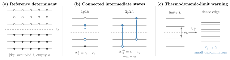
A one-body residual connects the reference to one-particle–one-hole states, while a normal-ordered two-body residual also reaches two-particle–two-hole states. At finite $L$ the denominators are discrete; near a gapless Fermi surface their spacing shrinks as the thermodynamic limit is approached.

Bosonic Occupation Enhancements

For bosons, occupation-number states replace a filled Fermi sea. If one mode has occupation $N_0$,

$$a_0 \lvert N_0\rangle = \sqrt{N_0} \lvert N_0-1\rangle,$$

and

$$a_0^\dagger a_0^\dagger a_0a_0 \lvert N_0\rangle = N_0(N_0-1) \lvert N_0\rangle.$$

The square-root factors change perturbative counting. A contact vertex may carry a small coefficient $g/\mathcal V$, yet replacing one or more condensate operators by their macroscopically occupied contribution produces factors of $\sqrt{N_0}$.

For example,

$$\frac{g}{2\mathcal V} \langle a_0^\dagger a_0^\dagger a_0a_0 \rangle = \frac{g}{2\mathcal V} N_0(N_0-1).$$

At fixed condensate density

$$n_0 = \frac{N_0}{\mathcal V},$$

this contribution is $O(\mathcal V)$ rather than a small finite correction:

$$\frac{g}{2\mathcal V} N_0(N_0-1) \sim \frac12 g n_0^2 \mathcal V.$$

Why the ideal condensate is not the final reference

In a symmetry-breaking displacement,

$$a_0 = \sqrt{N_0} + \delta a_0,$$

expanding an interacting Bose gas directly around the ideal condensate produces a hierarchy:

• a zero-body condensate energy of order $\mathcal V$;
• linear fluctuation terms of order $\sqrt{\mathcal V}$ unless the background satisfies its stationarity equation;
• quadratic normal and anomalous terms that mix creation and annihilation operators;
• cubic and quartic residual interactions.

A number-conserving construction organizes the condensate mode differently but retains the same occupation-enhanced power counting.

Gross–Pitaevskii Equation owns the stationary background. Bogoliubov Theory owns the exact diagonalization of the quadratic fluctuation Hamiltonian and the dilute-gas control parameter.

The perturbative lesson is general:

Macroscopic occupation promotes selected interaction terms to leading order. They must be absorbed into the reference before the remaining residual interaction is counted as small.

Bosons have no Pauli blocking, so low-energy phase space and zero modes can be more infrared sensitive than the corresponding fermionic determinant expansion.

Low-Order Energy and State Corrections

For a nondegenerate finite-volume reference, ordinary Rayleigh–Schrödinger theory gives

$$E^{(1)} = \langle\Phi|V|\Phi\rangle.$$

If the perturbation has been defined as a purely nonconstant normal-ordered residual, then

$$E^{(1)}=0$$

by bookkeeping. The reference expectation value has already been placed in $E_{\mathrm{ref}}$. If a constant remains in $V$, it must be retained.

The second-order energy is

$$E^{(2)} = \sum_{\nu\neq0} \frac{ \lvert\langle\nu|V|\Phi\rangle\rvert^2 }{ E_{\mathrm{ref}}-E_\nu^{(0)} }.$$

Using excitation rank,

$$\begin{aligned} E^{(2)} &= \sum_{i,a} \frac{ \lvert u_{ai}\rvert^2 }{ \epsilon_i-\epsilon_a } \\ &\quad + \frac14 \sum_{i,j,a,b} \frac{ \lvert\overline v_{ab;ij}\rvert^2 }{ \epsilon_i+\epsilon_j -\epsilon_a-\epsilon_b }. \end{aligned}$$

The first term vanishes for a canonical Hartree–Fock reference. The second is the familiar second-order correlation-energy structure used across electronic, nuclear, and condensed-matter calculations.

Why the factor is one quarter

With unrestricted labels,

$$\lvert\Phi_{ij}^{ab}\rangle = -\lvert\Phi_{ji}^{ab}\rangle = -\lvert\Phi_{ij}^{ba}\rangle.$$

The unrestricted sum counts each unordered occupied pair twice and each unordered unoccupied pair twice. The factor $1/4$ removes the fourfold duplication. If one sums only over $i<j$ and $a<b$, no such prefactor is needed.

Sign of the second-order energy

If every connected intermediate determinant lies above the reference in $H_0$, then

$$E_{\mathrm{ref}}-E_\nu^{(0)}<0.$$

Hence

$$E^{(2)}\leq0$$

for the displayed Hermitian coupling. This sign is a useful check, not a theorem for excited-state branches, unstable references, energy-dependent perturbation theories, or effective interactions with different bookkeeping.

First-order state correction

In intermediate normalization,

$$\begin{aligned} \lvert\Psi^{(1)}\rangle &= \sum_{i,a} \frac{ u_{ai} }{ \epsilon_i-\epsilon_a } \lvert\Phi_i^a\rangle \\ &\quad + \frac14 \sum_{i,j,a,b} \frac{ \overline v_{ab;ij} }{ \epsilon_i+\epsilon_j -\epsilon_a-\epsilon_b } \lvert\Phi_{ij}^{ab}\rangle. \end{aligned}$$

This formula makes the control problem visible. A small matrix element is not enough; every ratio of a connected matrix element to its energy denominator must be examined, together with the number of states carrying comparable ratios.

Volume Counting in a Uniform Fermi System

Consider spinful fermions in a periodic volume $\mathcal V$:

$$H_0 = \sum_{\mathbf k,\sigma} \epsilon_{\mathbf k} c_{\mathbf k\sigma}^\dagger c_{\mathbf k\sigma}.$$

A translation-invariant two-body interaction can be written as

$$\begin{aligned} V &= \frac{1}{2\mathcal V} \sum_{\mathbf k,\mathbf k',\mathbf q} \sum_{\sigma,\sigma'} v(\mathbf q) \\ &\quad\times c_{\mathbf k+\mathbf q,\sigma}^\dagger c_{\mathbf k'-\mathbf q,\sigma'}^\dagger c_{\mathbf k',\sigma'} c_{\mathbf k,\sigma}. \end{aligned}$$

The factor $1/\mathcal V$ comes from finite-volume plane-wave normalization. Momentum conservation has already removed one momentum sum.

At second order, a representative two-particle–two-hole contribution has the structure

$$\begin{aligned} E^{(2)} &= -\frac{1}{4\mathcal V^2} \sum_{\mathbf k,\mathbf k',\mathbf q} \frac{ n_{\mathbf k} n_{\mathbf k'} \left(1-n_{\mathbf k+\mathbf q}\right) \left(1-n_{\mathbf k'-\mathbf q}\right) }{ \Delta\epsilon } \\ &\quad\times \left| \overline v( \mathbf k+\mathbf q, \mathbf k'-\mathbf q; \mathbf k,\mathbf k' ) \right|^2, \end{aligned}$$

with spin sums suppressed and

$$\Delta\epsilon = \epsilon_{\mathbf k+\mathbf q} +\epsilon_{\mathbf k'-\mathbf q} -\epsilon_{\mathbf k} -\epsilon_{\mathbf k'}.$$

The prefactor assumes unrestricted antisymmetrized pair labels; equivalent conventions rearrange numerical factors.

Why an extensive answer can emerge

For a regular short-range interaction:

• each two-body matrix element contributes $1/\mathcal V$;
• its square contributes $1/\mathcal V^2$;
• the three independent momentum sums each contribute $O(\mathcal V)$;
• a regular denominator is $O(1)$.

Therefore

$$E^{(2)} = O(\mathcal V).$$

The energy density

$$e^{(2)} = \frac{E^{(2)}}{\mathcal V}$$

can have a finite thermodynamic limit.

This counting fails if the interaction or denominator is singular. Long-range Coulomb behavior, nesting, van Hove singularities, low-dimensional kinematics, or a soft collective mode can change the power or introduce logarithms.

Pauli blocking is part of the phase space

The occupation factors require both initial states to be occupied and both final states to be empty. They are not optional decorations. They:

• restrict intermediate states to allowed particle–hole configurations;
• eliminate many apparent low-energy processes;
• make the geometry of the Fermi surface central;
• change with temperature and with the chosen reference state.

The canonical excitation treatment develops this kinematics in full. Here it determines which perturbative denominators actually occur.

Degeneracy Is the Rule, Not the Exception

Many-body systems produce several kinds of degeneracy.

Symmetry multiplets

Spin, translation, point-group, or other symmetries can produce exact multiplets. Work in irreducible sectors, then apply degenerate perturbation theory inside any remaining multiplet.

Open shells

In a finite Fermi system, several orbitals can share the Fermi energy. Different ways of occupying the open shell produce degenerate determinants. Selecting one determinant and inserting zero denominators into a nondegenerate formula is invalid.

The correct first-order problem is

$$PVP,$$

where $P$ spans every determinant in the degenerate model space that is connected at the relevant order.

Near-degenerate manifolds

If

$$\left| E_\alpha^{(0)}-E_\beta^{(0)} \right| \lesssim \lambda \left| V_{\alpha\beta} \right|,$$

then the two states must be treated together even if their unperturbed energies are not exactly equal.

To second order, the model-space structure is

$$\begin{aligned} H_{\mathrm{eff}} &= E_0P +\lambda PVP \\ &\quad + \lambda^2 PVQ \frac{1}{ E_0-QH_0Q } QVP + \cdots, \end{aligned}$$

where $Q=I-P$. This formula only marks the route; the effective-Hamiltonian pages own its derivation, energy dependence, Hermitization, and operator transformation.

Gapless thermodynamic spectra

At a Fermi surface or in a system with Goldstone modes, the lowest excitation energy decreases with $L$. A finite system can have a unique ground state while

$$\Delta_L \longrightarrow 0$$

as $L\to\infty$.

The ordinary isolated-eigenvalue hypothesis is then not uniform in volume. One should not conclude that all perturbation theory fails. One should instead identify:

• which states are connected by $V$;
• whether phase space compensates small denominators;
• whether the energy density remains finite;
• which channel requires resummation;
• whether a different quasiparticle or broken-symmetry reference is needed.

Dense spectra do not make every state relevant

The full many-body level spacing can be exponentially small in volume. A local few-body perturbation does not couple every pair of eigenstates with equal strength. Symmetry, locality, momentum conservation, and excitation rank strongly restrict connectivity.

The relevant control quantity is not the smallest spacing anywhere in the spectrum. It is the ratio of matrix element to spacing within the states and sectors actually connected to the target.

Linked-Cluster Structure

An extensive system exposes a problem hidden in few-level perturbation theory. Naively expanding the state produces products of independent excitations in distant regions. Individual terms can scale as powers of volume larger than one, even though the exact ground-state energy should scale only as $\mathcal V$.

The cure is not to discard large terms by inspection. It is to organize the expansion so disconnected contributions cancel or exponentiate.

Imaginary-time projection

For a finite system with

$$\langle\Psi_0|\Phi\rangle\neq0,$$

define

$$Z_\Phi(\beta,\lambda) = \langle\Phi| e^{-\beta H(\lambda)} |\Phi\rangle.$$

As $\beta\to\infty$,

$$Z_\Phi \sim \lvert\langle\Psi_0|\Phi\rangle\rvert^2 e^{-\beta E_0(\lambda)}.$$

Hence

$$E_0(\lambda) = -\lim_{\beta\to\infty} \frac{1}{\beta} \ln Z_\Phi(\beta,\lambda).$$

After dividing by the corresponding reference factor,

$$\frac{ Z_\Phi(\beta,\lambda) }{ Z_\Phi(\beta,0) } = \left\langle \mathcal T_\tau \exp\!\left[ -\lambda \int_0^\beta d\tau\, V_I(\tau) \right] \right\rangle_0.$$

The logarithm has the cumulant expansion

$$\begin{aligned} \ln \frac{ Z_\Phi(\beta,\lambda) }{ Z_\Phi(\beta,0) } &= \sum_{n=1}^{\infty} \frac{(-\lambda)^n}{n!} \\ &\quad\times \int_0^\beta d\tau_1\cdots d\tau_n\, \left\langle \mathcal T_\tau V_I(\tau_1)\cdots V_I(\tau_n) \right\rangle_{0,\mathrm c}. \end{aligned}$$

Only connected cumulants appear in the logarithm. For a Gaussian Slater reference, Wick’s theorem further resolves these cumulants into linked contraction topologies. The next page develops that diagrammatic language.

Why disconnected vacuum pieces disappear

Suppose two subsystems do not interact:

$$H_{AB}=H_A+H_B, \qquad \lvert\Phi_{AB}\rangle = \lvert\Phi_A\rangle \otimes \lvert\Phi_B\rangle.$$

Then

$$Z_{AB} = Z_AZ_B.$$

Taking the logarithm gives

$$\ln Z_{AB} = \ln Z_A+\ln Z_B,$$

so

$$E_{AB} = E_A+E_B.$$

Products in which one perturbation acts independently in $A$ and another in $B$ occur in the expansion of $Z_{AB}$. They cancel from $\ln Z_{AB}$ through the cumulant subtraction. This is the physical core of the linked-cluster theorem.

Size consistency and size extensivity

Two related terms should be distinguished:

• size consistency: two infinitely separated subsystems have an energy equal to the sum of their separately calculated energies;
• size extensivity: the energy scales linearly with the number of repeated noninteracting units.

A properly linked perturbative energy is size extensive order by order under its stated assumptions. An arbitrary truncation of the many-body wavefunction need not be, even if it is variational.

What linked does not guarantee

Linked-cluster organization does not guarantee:

• convergence of the series;
• absence of infrared or ultraviolet divergences;
• a correct reference phase;
• conservation laws after an inconsistent truncation;
• accurate spectra or wavefunctions;
• validity at a singular thermodynamic point.

It fixes disconnected volume scaling. Other failures need other reorganizations.

Energy, State, and Observable Expansions Differ

The exact energy density can remain smooth even when the exact many-body state becomes nearly orthogonal to the reference.

Fidelity susceptibility

For a normalized nondegenerate ground state,

$$\lvert\Psi_0(\lambda)\rangle = \lvert\Psi_0(0)\rangle + \lambda \lvert\Psi_0^{(1)}\rangle + \cdots.$$

The fidelity has the small-$\lambda$ form

$$\left| \langle \Psi_0(0) | \Psi_0(\lambda) \rangle \right|^2 = 1-\lambda^2\chi_F+O(\lambda^3),$$

with

$$\chi_F = \sum_{\nu\neq0} \frac{ \lvert \langle\nu|V|0\rangle \rvert^2 }{ \left( E_\nu^{(0)}-E_0^{(0)} \right)^2 }.$$

Because the denominator is squared, state overlap is more infrared sensitive than the second-order energy. In an extended regular system, $\chi_F$ often grows at least as $\mathcal V$. For fixed nonzero $\lambda$, the global overlap can vanish as $\mathcal V\to\infty$ even while local observables change smoothly.

Quantum Phase Transitions owns fidelity susceptibility as a critical diagnostic. Here it shows why wavefunction closeness is too strong a requirement for bulk perturbation theory.

Orthogonality catastrophe

A local scattering potential can change the phase shift of every occupied orbital near a Fermi surface. The overlap of the old and new Fermi seas then decays as a power of system size:

$$\left| \langle\Phi_0|\Psi_0\rangle \right| \sim L^{-\alpha}, \qquad \alpha>0.$$

The ground-state energy shift can remain finite. Thus a state expansion about $\lvert\Phi_0\rangle$ can have a singular norm while selected energy differences and local responses remain meaningful after resummation.

Local observables from sources

For an observable $O$, introduce

$$H(J) = H+JO.$$

When differentiability and normalization conditions hold,

$$\langle O\rangle = \left. \frac{\partial E_0(J)}{\partial J} \right|_{J=0}.$$

Expanding the linked energy in both $\lambda$ and $J$ organizes connected contributions to the observable. This is generally safer than inserting an unnormalized truncated state into an expectation value without its norm and operator corrections.

Effective operators matter

If high-energy states are eliminated by a unitary or similarity transformation, observables must be transformed with the same map:

$$O_{\mathrm{eff}} = P e^S O e^{-S} P.$$

Using an effective Hamiltonian with the bare projected observable can miss contributions at the same perturbative order as the energy correction.

Infrared Problems

An infrared problem arises when low-energy modes make denominators, phase-space integrals, or repeated scattering singular.

A small denominator is not sufficient

One must combine:

• the denominator’s low-energy scaling;
• the matrix element’s momentum dependence;
• the density of intermediate states;
• Pauli or Bose occupation factors;
• conservation laws and symmetry;
• cancellations among terms.

A gapless spectrum can still have finite perturbative coefficients. Conversely, a logarithmic phase-space enhancement can invalidate fixed-order theory even when no single finite-volume denominator is exactly zero.

Cooper logarithm

Near a Fermi surface, repeated scattering of opposite-momentum fermions in an attractive pair channel produces

$$\int_E^\Lambda \frac{d\xi}{\xi} = \ln\!\left( \frac{\Lambda}{E} \right).$$

The effective expansion parameter becomes

$$\lvert g\rvert \nu_{\mathrm F} \ln\!\left( \frac{\Lambda}{E} \right),$$

not merely $\lvert g\rvert\nu_{\mathrm F}$. For any fixed attraction, the logarithm grows as $E\to0$. Repeated pair scattering must be resummed, and the normal Fermi-sea reference becomes unstable.

The resulting bound-state and BCS derivations belong to BCS Mean-Field Theory. The lesson here is that an arbitrarily weak bare interaction can be nonperturbative at a sufficiently low scale.

Long-range Coulomb interaction

For a three-dimensional Coulomb interaction,

$$v(q) \propto \frac{1}{q^2}.$$

Small momentum transfer enhances direct perturbative terms. In the high-density electron gas, fixed-order contributions contain infrared singularities even though the final correlation energy is well defined after the leading ring terms are summed.

Random Phase Approximation owns that resummation, screening, and the collective plasmon pole. This example shows why nominal order in the coupling can differ from the physically leading infrared order.

One-dimensional Fermi systems

In one dimension, particle–hole phase space and repeated forward or backscattering generate strong logarithmic structure. The ordinary quasiparticle expansion around a free Fermi sea is generally not the correct low-energy organization. Luttinger Liquid Preview owns the replacement by collective bosonic modes.

Goldstone and critical modes

If a mode has

$$\omega_{\mathbf q} \longrightarrow 0$$

as $\mathbf q\to0$, loop or intermediate-state integrals can be infrared enhanced. Dimension and temperature determine whether the integral is finite. Near a continuous phase transition, a diverging correlation length makes fixed-order expansion around a noncritical reference unreliable.

Large-$N$, renormalization-group, self-consistent, or symmetry-adapted methods can reorganize these fluctuations, but each requires its own control parameter.

Finite size and temperature as regulators

A finite box supplies a lowest nonzero momentum of order $2\pi/L$. Temperature supplies Matsubara scales and smears a Fermi surface over energies of order $k_{\mathrm B}T$. Perturbative expressions may therefore contain

$$\ln L, \qquad \ln\!\left( \frac{\Lambda}{k_{\mathrm B}T} \right), \qquad L^\gamma.$$

These dependences diagnose the infrared problem. They should not be hidden by reporting only one finite size or temperature.

Ultraviolet Problems

Short-distance singularities are logically separate from infrared denominators.

Continuum contact interactions

A formal interaction

$$g \int d^d x\, \psi^\dagger_\uparrow \psi^\dagger_\downarrow \psi_\downarrow \psi_\uparrow$$

does not guarantee that perturbative momentum integrals are finite. In two and three dimensions, the bare coupling generally depends on the ultraviolet regulator and must be matched to a scattering observable.

Expanding in a cutoff-dependent bare $g$ and then sending the cutoff to infinity can produce meaningless coefficients. Match or renormalize first, then identify the physical small parameter.

Lattice models

A lattice supplies a finite Brillouin zone and removes continuum ultraviolet momentum divergence. It does not remove:

• strong local-coupling problems;
• dense low-energy spectra;
• infrared singularities;
• truncation error from omitted bands or orbitals;
• regulator dependence introduced by a later continuum limit.

Effective interactions

Screened, retarded, or low-energy interactions already contain eliminated physics. Their perturbative order must be defined relative to the effective theory, not inferred from the number of microscopic vertices that produced them.

Thermodynamic-Limit Caveats

For finite volume,

$$E_0(\lambda,\mathcal V) = \sum_{n=0}^{\infty} \lambda^n E^{(n)}(\mathcal V)$$

may exist within a volume-dependent radius. The desired bulk quantity is

$$e_0(\lambda) = \lim_{\mathcal V\to\infty} \frac{ E_0(\lambda,\mathcal V) }{ \mathcal V }.$$

It is not automatic that

$$\begin{aligned} e_0(\lambda) &= \sum_{n=0}^{\infty} \lambda^n \lim_{\mathcal V\to\infty} \frac{ E^{(n)}(\mathcal V) }{ \mathcal V }. \end{aligned}$$

Interchanging the sum and limit requires uniform control that often fails near gapless points and phase transitions.

Nonanalytic bulk behavior

At finite volume, avoided crossings can keep the ground-state energy analytic. In the thermodynamic limit, distinct phases can cross and produce nonanalyticity. Pairing can generate a scale

$$\Delta \sim \Lambda \exp\!\left[ -\frac{1}{ \lvert g\rvert\nu_{\mathrm F} } \right],$$

whose Taylor series at $g=0$ vanishes term by term. No finite-order expansion around the normal state produces this scale.

Correct extensive scaling is necessary, not sufficient

A coefficient proportional to $\mathcal V$ has the right bulk scaling. It can still:

• diverge with the infrared cutoff;
• depend on an ultraviolet cutoff;
• grow factorially with order;
• describe the wrong phase;
• violate a conservation law under inconsistent truncation.

Boundary conditions and shell effects

Finite-size coefficients can oscillate with particle number or boundary twist because the last occupied shell changes. Useful strategies include:

• closed-shell sequences;
• symmetry-resolved boundary conditions;
• twist averaging for numerical studies;
• explicit finite-size scaling;
• comparing several shape sequences rather than one box.

The extrapolation protocol is part of the perturbative result.

Adiabatic Switching and Its Limits

One formal route to the interacting state turns on the interaction slowly:

$$H_\eta(t) = H_0 + \lambda e^{\eta t} V, \qquad t\leq0, \quad \eta>0.$$

Schematically,

$$\lvert\Psi_0\rangle \propto \lim_{\eta\to0^+} \frac{ U_\eta(0,-\infty) \lvert\Phi\rangle }{ \langle\Phi| U_\eta(0,-\infty) |\Phi\rangle }.$$

The denominator removes disconnected vacuum factors and a divergent phase in the standard construction. The limit requires that the chosen state be connected to the target branch without an obstructing level crossing or uncontrolled degeneracy.

In a many-body system, adiabatic switching can fail or become subtle because:

• the gap closes with volume;
• the reference and target states become orthogonal;
• the interaction changes the phase;
• an infinitesimal source is needed to select a broken-symmetry branch;
• limits $\eta\to0$, $\mathcal V\to\infty$, and $T\to0$ do not commute.

The formal switching prescription does not repair a poor reference by itself.

Finite-Temperature Expansion

At temperature $T=1/(k_{\mathrm B}\beta)$, the central object is a trace rather than one eigenstate:

$$Z(\lambda) = \operatorname{Tr} e^{-\beta(H_0+\lambda V)}.$$

In the interaction representation,

$$\frac{Z(\lambda)}{Z_0} = \left\langle \mathcal T_\tau \exp\!\left[ -\lambda \int_0^\beta d\tau\, V_I(\tau) \right] \right\rangle_0.$$

The grand potential or free energy is a logarithm:

$$\Omega(\lambda) = -\frac{1}{\beta} \ln Z(\lambda).$$

Its perturbative expansion therefore contains connected thermal cumulants. Fermi–Dirac or Bose–Einstein occupation factors replace zero-temperature step functions.

Finite temperature can regularize some zero-temperature singularities, but it introduces:

• Matsubara zero modes for bosons;
• thermal phase transitions;
• order-of-limits questions between $T\to0$ and $\mathcal V\to\infty$;
• analytic continuation if real-frequency response is required.

The full thermal Green-function machinery belongs to the later field-theory bridge and diagrammatic treatment.

When to Reorganize the Expansion

Diagnostic	Likely response
isolated reference with regular denominators	ordinary finite-order perturbation theory
exact or near degeneracy among a few states	degenerate or quasi-degenerate model space
strong mean one-body field	absorb it into Hartree or Hartree–Fock $H_0$
stable condensate with weak depletion	Gross–Pitaevskii plus Bogoliubov expansion
logarithmic pair channel	Cooper or BCS resummation
long-range density feedback	RPA or a conserving screened expansion
large internal component number	saddle and $1/N$ hierarchy
large local repulsion with a low-energy manifold	inverse-coupling effective Hamiltonian
repeated short-range scattering	two-body $T$ matrix or ladder resummation
scale-dependent logarithms across many decades	renormalization-group treatment
no small parameter and competing references	cross-method benchmarks or nonperturbative numerics

Resummation is not “including more terms” in the abstract. It identifies a family of terms enhanced by a physical mechanism and treats that family to all orders.

A Reliable Workflow

1. Specify the target. State whether the calculation concerns an energy, state, free energy, response, or effective operator.
2. Regulate first. Fix volume, boundary conditions, basis cutoff, particle sector, and ensemble.
3. Define the split. Write $H_0$, $V$, counterterms, and the physical value of $\lambda$.
4. Identify the reference. State its symmetries, occupations, quasiparticles, and whether it is optimized.
5. Normal order consistently. Keep induced zero- and one-body terms and declare matrix-element conventions.
6. Classify connected intermediates. Use excitation rank, momentum, spin, and symmetry before summing.
7. Audit degeneracy. Build a model space whenever connected gaps are comparable to matrix elements.
8. Check N and volume scaling. Track powers from matrix elements, sums, conservation laws, and normalization.
9. Organize linked quantities. Use logarithms, cumulants, or a proven linked diagram expansion for energies and free energies.
10. Inspect infrared behavior. Vary $L$, $T$, and external scales; look for logs, powers, or soft denominators.
11. Inspect ultraviolet behavior. Match bare parameters and verify cutoff independence of physical coefficients.
12. Test identities. Check Hermiticity, antisymmetry, conservation laws, sum rules, and known limiting signs.
13. Compare references and orders. Stability under nearby partitions is useful evidence, though not a rigorous error bar.
14. Benchmark. Use exact diagonalization, quantum Monte Carlo, coupled cluster, tensor networks, or experiment where appropriate.
15. State the limit order. Report how $\mathcal V\to\infty$, $T\to0$, cutoff removal, and adiabatic switching are taken.

Common Mistakes

• Calling the bare coupling the expansion parameter without including density of states and denominators.
• Taking the continuum or thermodynamic limit before defining finite-volume intermediate states.
• Using a single determinant inside an exactly degenerate open shell.
• Treating the smallest spacing anywhere in the spectrum as relevant without checking matrix elements and symmetry.
• Forgetting induced zero- and one-body terms after reference normal ordering.
• Omitting the mean-field counterterm from the residual interaction.
• Mixing bare and antisymmetrized two-body matrix-element prefactors.
• Counting a one-particle–one-hole state as a change in total particle number.
• Applying the Hartree–Fock Brillouin condition to a nonstationary reference.
• Assuming every second-order ground-state correction is negative without checking the branch and denominators.
• Interpreting an extensive number of intermediate states as a failure before doing volume normalization.
• Keeping disconnected products in an energy and obtaining powers larger than $\mathcal V$.
• Assuming linked-cluster organization guarantees convergence.
• Using a truncated, unnormalized state to evaluate observables without norm corrections.
• Demanding nonzero global overlap as a condition for smooth local physics in the thermodynamic limit.
• Expanding through a Cooper, screening, Kondo, or critical logarithm instead of resumming the enhanced channel.
• Treating temperature or finite size as a cure rather than an infrared regulator whose removal must be studied.
• Removing a continuum cutoff while holding a regulator-dependent bare contact coupling fixed.
• Using an effective Hamiltonian with untransformed observables.
• Reporting one closed-shell finite size as the thermodynamic limit.

Exercises

1. Excitation-rank selection. Let $\lvert\Phi\rangle$ be a determinant, and let

   $$V^{[1]} = \sum_{pq} u_{pq} \{a_p^\dagger a_q\}_{\Phi}.$$

   Show that $V^{[1]}\lvert\Phi\rangle$ contains only one-particle–one-hole states. Why does its reference expectation value vanish?

Solution

Reference normal ordering rewrites every operator in terms of particle and hole quasiparticle creators and annihilators. Acting on $\lvert\Phi\rangle$, any term containing a quasiparticle annihilator vanishes. The only surviving nonconstant one-body terms have one unoccupied creator and one occupied annihilator:

$$V^{[1]}\lvert\Phi\rangle = \sum_{i,a} u_{ai} a_a^\dagger a_i \lvert\Phi\rangle.$$

Thus

$$V^{[1]}\lvert\Phi\rangle = \sum_{i,a} u_{ai} \lvert\Phi_i^a\rangle.$$

Every one-particle–one-hole determinant is orthogonal to the reference, so

$$\langle\Phi| V^{[1]} |\Phi\rangle = 0.$$

The zero-body contraction was separated before $V^{[1]}$ was defined.

2. Second-order pair factor. Starting from unrestricted sums over occupied $i,j$ and unoccupied $a,b$, explain why

   $$E^{(2)}_{2p2h} = \frac14 \sum_{ijab} \frac{ \lvert\overline v_{ab;ij}\rvert^2 }{ \epsilon_i+\epsilon_j-\epsilon_a-\epsilon_b }$$

   contains a factor $1/4$. Rewrite it using ordered pairs.

Solution

Antisymmetry gives

$$\overline v_{ab;ij} = -\overline v_{ba;ij} = -\overline v_{ab;ji}.$$

The squared magnitude is unchanged under $i\leftrightarrow j$ and $a\leftrightarrow b$. An unrestricted sum therefore counts the same pair excitation four times:

$$(i,j;a,b), \quad (j,i;a,b), \quad (i,j;b,a), \quad (j,i;b,a).$$

The prefactor removes this duplication. With ordered pairs,

$$E^{(2)}_{2p2h} = \sum_{i<j} \sum_{a<b} \frac{ \lvert\overline v_{ab;ij}\rvert^2 }{ \epsilon_i+\epsilon_j-\epsilon_a-\epsilon_b }.$$

Both formulas assume normalized determinants and the same antisymmetrized matrix-element convention.

3. Volume counting. In a periodic volume $\mathcal V$, suppose a two-body plane-wave matrix element scales as $\mathcal V^{-1}$. A second-order connected energy has three independent momentum sums and two vertices. Determine its leading volume scaling when denominators are regular.

Solution

Each vertex contributes

$$\mathcal V^{-1},$$

so two vertices contribute $\mathcal V^{-2}$. Each independent momentum sum contains a number of states proportional to $\mathcal V$. Three sums therefore contribute $\mathcal V^3$. A regular denominator is $O(1)$, giving

$$E^{(2)} \sim \mathcal V^3 \mathcal V^{-2} = \mathcal V.$$

Thus

$$\frac{E^{(2)}}{\mathcal V} = O(1).$$

If $v(q)$ or the denominator is singular at small $q$, this elementary counting must be refined.

4. Linked cancellation for separated systems. Let

   $$Z_A = 1+\lambda A_1+\lambda^2A_2+O(\lambda^3),$$

   and define $Z_B$ analogously. Expand $\ln(Z_AZ_B)$ through second order. Show explicitly that the cross term $A_1B_1$ does not survive.

Solution

First,

$$\begin{aligned} Z_AZ_B &= 1 +\lambda(A_1+B_1) \\ &\quad +\lambda^2 \left( A_2+B_2+A_1B_1 \right) + O(\lambda^3). \end{aligned}$$

Using

$$\ln(1+x) = x-\frac{x^2}{2}+O(x^3),$$

gives

$$\begin{aligned} \ln(Z_AZ_B) &= \lambda(A_1+B_1) \\ &\quad +\lambda^2 \left[ A_2-\frac{A_1^2}{2} + B_2-\frac{B_1^2}{2} \right] + O(\lambda^3). \end{aligned}$$

The product $A_1B_1$ from $Z_AZ_B$ is canceled by the cross term in

$$-\frac12 \lambda^2(A_1+B_1)^2.$$

Equivalently,

$$\ln(Z_AZ_B) = \ln Z_A+\ln Z_B.$$

5. Open-shell degeneracy. Two orbitals $p$ and $q$ have the same unperturbed energy, and one fermion occupies the two-dimensional shell. In the basis $\{\lvert p\rangle,\lvert q\rangle\}$, the perturbation is

   $$PVP = \begin{pmatrix} A & B\\ B^\ast & C \end{pmatrix}.$$

   Find the first-order shifts and explain why using either diagonal element alone is not perturbation theory for the degenerate problem.

Solution

The first-order shifts are the eigenvalues of $PVP$:

$$E_\pm^{(1)} = \frac{A+C}{2} \pm \sqrt{ \left( \frac{A-C}{2} \right)^2 + \lvert B\rvert^2 }.$$

The corresponding zeroth-order states are the eigenvectors of this matrix. Choosing $\lvert p\rangle$ and assigning the shift $A$ ignores mixing by $B$; choosing $\lvert q\rangle$ and assigning $C$ gives a different arbitrary answer. The unperturbed Hamiltonian did not select either basis vector inside the degenerate shell. The perturbation must be diagonalized there first.

6. Cooper logarithm. Evaluate

   $$I(E) = \nu_{\mathrm F} \int_E^\Lambda \frac{d\xi}{\xi}, \qquad 0<E<\Lambda.$$

   At what scale does a nominally weak attraction $g$ make $|g|I(E)$ order one?

Solution

The integral is

$$I(E) = \nu_{\mathrm F} \ln\!\left( \frac{\Lambda}{E} \right).$$

The fixed-order expansion fails when

$$\lvert g\rvert \nu_{\mathrm F} \ln\!\left( \frac{\Lambda}{E} \right) \sim1.$$

Solving parametrically,

$$E_\ast \sim \Lambda \exp\!\left[ -\frac{1}{ \lvert g\rvert\nu_{\mathrm F} } \right].$$

This scale is nonanalytic at $g=0$. Numerical factors depend on the pairing convention and density-of-states normalization.

7. Energy versus fidelity denominators. Compare

   $$E^{(2)} = -\sum_{\nu\neq0} \frac{|V_{\nu0}|^2}{\Delta_\nu}$$

   with

   $$\chi_F = \sum_{\nu\neq0} \frac{|V_{\nu0}|^2}{\Delta_\nu^2}, \qquad \Delta_\nu>0.$$

   If low-energy states have spectral weight

   $$\sum_\nu |V_{\nu0}|^2 \delta(\omega-\Delta_\nu) \sim C\omega^s$$

   as $\omega\to0$, determine the infrared convergence conditions for both quantities.

Solution

At low energy,

$$E^{(2)}_{\mathrm{IR}} \sim -C \int_0 d\omega\, \omega^{s-1}.$$

This converges at the lower limit when

$$s>0.$$

The fidelity susceptibility behaves as

$$\chi_{F,\mathrm{IR}} \sim C \int_0 d\omega\, \omega^{s-2},$$

which converges only when

$$s>1.$$

Thus there is a range

$$0<s\leq1$$

for which the second-order energy is infrared finite while the state overlap is singular.

8. Order of limits. Suppose a finite-size energy-density coefficient behaves as

   $$e^{(2)}(L) = e_\infty^{(2)} + A\lambda^2\ln L.$$

   Can it define a finite second-order thermodynamic coefficient at fixed $\lambda\neq0$? What does the logarithm suggest?

Solution

At fixed nonzero $\lambda$,

$$\lim_{L\to\infty} e^{(2)}(L)$$

does not exist because of the logarithm. The finite-volume coefficient is well defined, but the thermodynamic limit is not uniform at this order.

The logarithm suggests that higher orders may contain powers such as

$$\lambda^n(\ln L)^{n-1}.$$

When

$$\lvert\lambda\ln L\rvert \sim1,$$

all such terms can become comparable. One should identify the physical channel generating the logarithm and resum or renormalize it before taking the bulk limit. The logarithm alone does not identify which resummation is correct.

Key Takeaways

• Many-body perturbation theory must specify a finite-volume reference, regulator, ensemble, and observable before taking limits.
• Normal ordering exposes the zero-, one-, and residual interaction pieces relative to that reference.
• One-body residuals create one-particle–one-hole states; two-body residuals can create two-particle–two-hole states.
• The second-order energy is controlled by matrix-element-to-denominator ratios and by the number of connected intermediate states.
• Hartree–Fock stationarity removes single excitations in the canonical partition but does not remove correlation.
• Plane-wave matrix elements shrink with volume while momentum sums grow; linked contributions can combine into an extensive energy.
• Exact and near degeneracy require a model space, not small-denominator substitution.
• Logarithms of a projection amplitude or partition function retain connected cumulants and enforce energy additivity.
• A smooth energy density does not require a nonvanishing global overlap with the reference state.
• Cooper pairing, Coulomb screening, one-dimensional kinematics, Goldstone modes, and criticality can invalidate fixed-order infrared counting.
• Continuum contact interactions require ultraviolet matching independently of infrared control.
• The thermodynamic limit can create nonanalytic scales and invalidate interchange of the perturbative sum with the volume limit.
• Resummation must be tied to a physically enhanced class of processes.

References

1. M. Gell-Mann and F. Low, “Bound States in Quantum Field Theory”, Physical Review 84, 350–354 (1951).
2. N. M. Hugenholtz, “Perturbation Theory of Large Quantum Systems”, Physica 23, 481–532 (1957).
3. J. Goldstone, “Derivation of the Brueckner Many-Body Theory”, Proceedings of the Royal Society A 239, 267–279 (1957).
4. M. Gell-Mann and K. A. Brueckner, “Correlation Energy of an Electron Gas at High Density”, Physical Review 106, 364–368 (1957).
5. L. N. Cooper, “Bound Electron Pairs in a Degenerate Fermi Gas”, Physical Review 104, 1189–1190 (1956).
6. P. W. Anderson, “Infrared Catastrophe in Fermi Gases with Local Scattering Potentials”, Physical Review Letters 18, 1049–1051 (1967).
7. F. J. Dyson, “Divergence of Perturbation Theory in Quantum Electrodynamics”, Physical Review 85, 631–632 (1952).
8. B. H. Brandow, “Linked-Cluster Expansions for the Nuclear Many-Body Problem”, Reviews of Modern Physics 39, 771–828 (1967).
9. A. L. Fetter and J. D. Walecka, Quantum Theory of Many-Particle Systems, Dover (2003).
10. J. W. Negele and H. Orland, Quantum Many-Particle Systems, Westview Press (1998).
11. G. D. Mahan, Many-Particle Physics, 3rd ed., Springer (2000).
12. A. A. Abrikosov, L. P. Gorkov, and I. E. Dzyaloshinski, Methods of Quantum Field Theory in Statistical Physics, Dover (1975).
13. I. Shavitt and R. J. Bartlett, Many-Body Methods in Chemistry and Physics, Cambridge University Press (2009).
14. P. Coleman, Introduction to Many-Body Physics, Cambridge University Press (2015).
15. T. Kato, Perturbation Theory for Linear Operators, 2nd ed., Springer (1995).